COINTEGRATION AND CAUSALITY BETWEEN TURKISH, IMPORTS AND GDP: A STRUCTURAL ANALYSIS

(1)

Eurasian Journal of Economics and Finance, 4(2), 2016, 91-100 DOI: 10.15604/ejef.2016.04.02.007

EURASIAN JOURNAL OF ECONOMICS AND FINANCE

http://www.eurasianpublications.com

C

OINTEGRATION AND

C

AUSALITY BETWEEN

T

URKISH

,

I

MPORTS AND

GDP:

A

S

TRUCTURAL

A

NALYSIS

Cagri Levent Uslu

Yeditepe University, TURKEY, Email: [email protected]

Abstract

The aim of this paper is to reveal the relation between imports and growth rate in Turkey for the period between the first quarter of 1998 and last quarter of 2014. The touchstone in Turkish economy is the January 24 regulations of 1980. The import led growth strategy of the Turkish economy switched to export led growth strategy after this date. It is an indisputable fact that trade openness triggered to the economic growth progress of Turkey. Yet, the issue should be further investigated. It is being argued by both scholars and politicians that the high growth rates in the mentioned period is achieved by importing raw materials and intermediate goods, thus, growth in Turkish economy has to be accompanied by the increase in imports and thus increase in trade deficit and current account deficit. In the literature, the relations between GDP growth and exports are intensively investigated, however, the relation between the second component of international trade, imports, and GDP growth did not attract that much attention. The main objective of this study is to reveal the presence and direction of Granger causality between Turkish Imports and GDP. The model to be employed in Granger causality (i.e. VAR vs. VECM) depends on whether the variables under question are stationary and/or co integrated. In testing the unit roots, we have followed the Augmented Dickey-Fuller (Dickey and Fuller, 1979) test which eventually became the standard practice in unit root testing. Next, to find the number of co integrating vectors Johansen Maximum Likelihood (Johansen and Juselius, 1990) test is employed.

Keywords: Granger Causality, Imports, GDP Growth

1. Introduction

(2)

Cagri Levent Uslu / Eurasian Journal of Economics and Finance, 4(2), 2016, 91-100

by shifting into labor intensive industries, (c) increasing capacity utilization rate, (d) increase in economies of scale, (e) increase in productivity by the effect of foreign competition.

The touchstone in Turkish economy is the January 24 regulations of 1980. The import led growth strategy of the Turkish economy switched to export led growth strategy after this date. At the beginning of this period, the ratio of trade volume to GDP, which is also interpreted as an indicator of openness, was 11.6%, whereas this figure was roughly 50% in 2014, reaching its peak of 56.5% in 2011 (CBRT, 2014). The effect of this ratio on economic growth is carried through the two components of trade; imports and exports. In calculating the GDP, exports has a positive contribution to the GDP, whereas, the negative sign of imports indicate a negative contribution.

It is an indisputable fact that trade openness positively conduced to the economic growth progress of Turkey. Yet, the issue should be further investigated. The trade balance (deficit) which constitutes the backbone of Current Account (CA) deficit is dramatically increased throughout the first fifteen years of the 2000s.The CA to GDP ratio increased from 0.2% in 2002 to 6% in 2014 with its peak of 9.7% in 2011 (CBRT, 2014).

It is being argued by both scholars and politicians that the high growth rates in the mentioned period is achieved by importing raw materials and intermediate goods, thus, growth in Turkish economy has to be accompanied by the increase in imports and thus increase in trade deficit and current account deficit.

In the literature, the relation between GDP growth and exports are intensively investigated, however, the relation between the second component of international trade, imports, and GDP growth did not attract that much attention. The contribution of this paper to the literature is to reveal the relation between imports and growth rate in Turkey for the period between the first quarter of 1998 and last quarter of 2014. The paper is organized as follows. In Section 2 we present a brief literature review and some selected papers. Section 3 is devoted to data and methodology. In Section 4, results of unit root, cointegration and Granger causality analysis are given. Finally, Section 5 is devoted to the conclusion.

2. Literature Review

Today it is a common view that economic growth cannot be realized without free trade. The term “trade” has two components, exports and imports; and both of these components have firm relations with domestic economic growth, which was and is still being intensively investigated by scholars. Thus, there is a large amount of empirical literature on investigating the causal relation between imports/exports and economic growth. These studies involve either investigating a single economy’s growth-trade relation or comparing the trade relations between two individual economies as well as investigating the relation between two groups of economies. Since the technical relationship between imports and the growth rate of the GDP is more complex than that of the exports and GDP growth relationship, in the literature, one can find some determinate number of empirical studies that try to analyze and reveal the causal relation between imports and GDP. On the contrary, much of the effort is spent to reveal the relation between exports and GDP (Ugur, 2008). Although in theory, there may be four types of relation between exports and GDP; (namely one way causalities from GDP growth to exports or from exports to GDP growth, a bi-directional causal relation and finally no relation), it is argued by most that there is a bi-directional causal relationship between exports and GDP growth implying that an increase in exports increases economic growth, and also economic growth increases volume of exports. In the literature, there are a limited number of studies that investigate these four types of relations between GDP and imports.

The period between 1930s and January 24, 1980 is the period in which Turkish economy applied import substitution policies. After then, liberalization of Turkish economy also changed the economic paradigm from import substitution to export led growth. Nevertheless, “should an economy promote trade in order to speed up the economic activity or should the economic growth trigger the trade” is the question that should be resolved.

(3)

i. The global competition pressure is likely to increase the quality of products and services and force the domestic producers to increase efficiency.

ii. For the economies in which domestic demand is low, the increase in exports may shift the exporting firm to the scope for economies of scale which in turn positively contributes to the allocative efficiency.

iii. These sectors may also generate positive externalities on the non-exports sector, through more efficient management styles and improved production techniques.

iv. Increase in exports triggers the boom in production, GDP and employment. Due to the short-run Keynesian macroeconomic model and specifically the multiplier effect, production and consumption will both rise, creating a positive feedback loop.

v. Finally, according to the recent “endogenous” growth theory, exports play an important role in increasing returns to scale and the spillover of this new production technique to other sectors are inevitable. Exports may increase long run growth by allowing the economy to specialize in those sectors in which R&D, human capital stock, is well enough to compete with the rest of the world. (Ghatak et. al. 1997; Singh and Konya, 2007; Simsek, 2003).

On the other hand, some authors (Mac Donald, 1994; Esfahani, 1991; Ram 1990) argue that imports also have a positive effect on economic growth and welfare. For those economies whose economic development strategies heavily rely on foreign capital investment, imports of capital goods are especially important. The key factor for foreign capital investment to be beneficial is, however, that it should be allocated to production of goods and services and not for consumption (Singh and Konya, 2007).

The very basic Keynesian economics states that GDP=Consumption + Investment + Government Spending + (Exports – Imports). As the negative sign of imports in the equation simply states, the increase in imports leads to a decrease in Gross Domestic Product. Thus, there should be some facts beyond the simple GDP equation that lead a positive relation between the GDP and imports. First, similar to the export sectors, increase in domestic competition due to the imports may stimulate domestic firms to increase quality, making these firms competitive in the global competition. Second, attaining high quality raw materials and intermediate goods may increase the factor productivity in domestic sectors.

This paper aims to reveal the Granger causality, if there is any, between economic growth and imports in Turkish economy. The recent course of Turkish economy is towards creating a large current account deficit. The rationale of this increasing current account deficit is explained by increase in imports of necessary capital goods for production and hence economic growth. Therefore, it is a good time to investigate whether imports are triggered by economic growth or the boom in imports causes economic growth.

In the literature, the only study that investigates the relation between imports and GDP in Turkey within the Granger causality framework is Ugur (2008). In this study, imports are firstseparatedsub-groups and then a multivariate VAR analysis is employed to reveal the Granger causality. It was concluded that there is a bi-directional relationship between GDP and investment goods import and raw materials import. Results also revealed that the relation between GDP and consumption goods import and other goods import is a unidirectional one.

Other studies related to the relation between GDP and imports in Turkish economy may be categorized into two: (a) studies that use imports in a trivariate VECM system in addition to exports and GDP, (b) studies that use imports as an exogenous variable in a bivariate VECM system in which the real focus is on the relation between exports and GDP.

(4)

employed a trivariate VECM model with imports, exports and GDP growth using the annual data from 1996 to 2006. Results indicated a bi-directional causality between exports, imports and GDP in the short-run and unidirectional causalities from exports to imports, from growth to exports and from growth to imports in the longrun. Finally, Bilgin and Sahbaz (2009) investigated the Granger causality between growth and export by using the monthly data between 1987 and 2007. Authors found a unidirectional causality from exports to economic growth.

3. Data and Methodology

The main aim of this study is to investigate the existence and direction of Granger causality between Turkish Imports and GDP. However, the model to be employed in Granger causality (i.e. VAR vs VECM) depends on whether the variables under question are stationary and/or cointegrated. In testing the unit roots, we have followed the Augmented Dickey-Fuller (Dickey and Fuller, 1979)test, which eventually became the standard practice in unit root testing. Next, the Johansen Maximum Likelihood (Johansen and Juselius, 1990)test is used to detect the number of cointegrating vectors, if there are any.

3.1. The unit root

Following Engle and Granger (1987), two series in hand have been tested for unit roots. Standard econometric models assume that variables are stationary. However many economic time series are non-stationary by nature. Employing ordinary least squares (OLS) methods to these non-stationary variables, thus,has a potential to end up with a spurious regression unless these variables are co-integrated (Granger and Newbold, 1974).

The most practiced unit root test is the ADF test. The simple Dickey-Fuller test may be applied only if the series have been generated by a first-order autoregressive process. On the contrarythe ADF test is stronger in a parametric correction for higher order autocorrelation. This strength originates from adding the lagged differences of the dependent variable to the right-hand side of the regression (Singh and Konya, 2007).

We start unit root test by the graphical examination of series, in order to figure out whether to include the intercept and time trend or not.

Figure 1. The logarithms of Turkish gross domestic product and imports

21 22 23 24 25 26 27 28 29 1998 Q1 1998 Q4 1999 Q3 2000 Q2 2001 Q1 2001 Q4 2002 Q3 2003 Q2 2004 Q1 2004 Q4 2005 Q3 2006 Q2 2007 Q1 2007 Q4 2008 Q3 20 09 Q2 2010 Q1 2010 Q4 2011 Q3 2012 Q2 2013 Q1 2013 Q4 2014 Q3 Ln GDP , Ln Im p Date

(5)

Figure 1 reveals that both LNGDP and LNIM are not evolving around a constant level but steadily increasing overtime; therefore levels of these variables were tested under the assumption that the data generating process has a time trend. The tests of first differences, on the contrary, are performed by including only the drift terms into the model.

3.2. Cointegration

It is a well-known fact in economics literature that most economic time series are non-stationary in their levels but stationary in their first (or second) differences. If two or more time series contain stochastic trends, that is, they are non-stationary in their levels, thus it is still possible that these time series have a long-run relation. In other words, the stochastic trends may be unique for these different non-stationary time series. The existence of such relation among variables is referred to as Cointegration. In the presence of unit roots, checking for Granger Causality requires tests for cointegration, and if there exists a cointegration vector, then it is safe to continue with causality.

Engle and Granger (1987) shown that the linear combination of two I(d) series like will in general be I(d). The existence of constant α where zt is I(d-b) and b>0 indicates that series yt and xt are cointegrated and denoted as CI(d,b). Specifically if, b=d=1 then they share the same stochastic trend and, thus, have a long-run equilibrium relationship. Engle and Granger (1987) have also shown that if there is a long-run equilibrium relationship (i.e. yt and xt are CI(1,1)) there must be a Granger causality either in the form of unidirectional or bi-directional.

In this study, the maximum likelihood estimation method of Johansen and Juselius (1990) is used to test for cointegration. The method is based on vector auto-regressive systems of nx1 vector of I(1) variables Xt

(1)

where … are nxn matrices of coefficients, p is the lag length and is the error term. Johansen cointegration test involves two statistics in testing the null hypothesis of no cointegration, namely the trace statistics and maximum eigenvalue (Max-L). These statistics are computed as follows:

(2)

)

(3)

where r is the number of distinct cointegrating vectors, and λ1…λN are the N squared correlations between the Xt-p and series. If the computed value of the statistic is below the critical value, then we cannot reject the null hypothesis of no cointegration (i.e. r=0).

3.3. Granger causality

The concept of Granger causality, first introduced by Granger (1969), may be defined as follows; if history of a time series X (Xt-1, Xt-2, …, X0), is proved to have significant statistical information, usually by t and F tests, about the future value of Y, then it is said that X Granger causes Y. In other words if X is causing Y, the change in X should take place before the change in Y, thus, the relation between the lagged values of X and present value of Y should be significant.

(6)

from the long-run cointegrating vectors, can be used to determine the direction of this causality (Masih and Masih, 1998).

If we assume that both Xt and Yt are stationary, Granger causality between these two variables may be shown by the following bivariate VAR model:

(4)

(5)

where, t and l denotes time period (t=1,β, ……,T) and the lag respectively and are white noise error terms, implying that their means are zero, have constant variances over time and are individually serially uncorrelated (Singh and Konya, 2006).

Four possible outcomes arise from the above equations related to the causality between X and Y. The first two may be categorized under the headline “one-way causality” or “unidirectional causality”. If not all ’s are zero in the first equation, but all ’s are zero in the second equation, then it is said that there is a one-way causality or unidirectional causality from X to Y, and denoted as . The opposite relation is also a unidirectional causality but this time from Y to X. In this case all ’s are zero in the first equation and not all ’s are zero in the second equation. The third type of causality may be called two-way or bidirectional causality between X and Y, denoted as . This type of causality occurs if neither all ’s nor all ’s are zero. Finally, the fourth type is situation in which no causality exists between X and Y, denoted as . In this case all ’s and ’s are zero.

Recent development of the Cointegration concepts indicate that VAR model specified in differences is valid only if the variables under study are not cointegrated. In such cases, VECM models should be used rather than a VAR in a standard Granger causality test (Engle and Granger, 1987). Since a cointegrating relationship was found between imports and GDP, following Engle and Granger (1987), the VECM for the Granger causality test to be estimated is written as follows:

(6)

(7)

where, GDPt is the gross domestic product and IMt is the import at time t, n is the number of lags to be included in the model, ECT refers to the error-correction term(s) derived from long-run cointegrating relationship and Ɛt is the white noise error term.

Given these two equations, Equation 6 will be employed to test the causal relation from imports to GDP and Equation 7 will be used to test the causality from GDP to imports. In addition to determining the direction of the causality, these equations may also be used to distinguish the short-run and the long-run relations between these variables. If variables are cointegrated, in the short run, deviations from this long-run equilibrium will feed back on the changes in the dependent variable in order to force the movement towards the long-run equilibrium. If this long-run equilibrium error directly drives the independent variable then it is responding to this feedback. If not, it is responding only to short-term shocks to the stochastic environment (Masih and Masih, 1998).

(7)

Granger causality itself is a two-step procedure. In the first step residuals from the long-run relationship are estimated. The short-long-run error correction model is estimated by adding the lagged residuals obtained in the first step to the exogenous variables (Mehrara and Firouzjaee, 2011).

4. Empirical Analysis 4.1. Unit root test

The existence of unit roots and identifying the order of integration for each variable has been carried out through the ADF test and results are presented in Table 1. The null hypothesis for each test is that the variable is non-stationary.

Table 1. ADF test results

Levels 1st differences

Variable Test

Statistics Critical Values

Test

Statistics Critical Values

LNGDP -2.34* (9)

1% level -4.161144 5% level -3.506374 10% level -3.183002

-3.75** (3)

LNIM -2,52* (5)

-2.98*** (4)

1% level -3.562669 5% level -2.918778 10% level -2.597285 Notes: a. * denotes that at all significance levels variables are non-stationary

b. ** denotes that at all significance levels variable is stationary c. *** denotes that at 5% and 10% levels variable is stationary

d. Numbers in parenthesis indicate the lags selected by AIC e. The critical values are obtained from Mac Kinnon (1996)

The ADF test rise two practical problems: first, the s(James, 1996)election of lag length; and second, the choice of exogenous variables. In solving the first problem Akaike Information Criterion (AIC) was used. Afterwards, residuals were tested for autocorrelation by employing Breusch-Godfrey Lagrange multiplier (LM) and it was made clear that residuals reflect no evidence of autocorrelation. The solution to the second problem, choice of exogenous variable, primarily relies on the graphical examination of the data. Levels and first differences of both variables were graphed and these graphs revealed that the levels have both intercept and time trend, whereas, the first differences have only intercept.

Results indicate that both variables are non-stationary at their levels at each level of significance. The results of the test at first differences are at the odds. Although the LNGDP is stationary at all levels of significance, the null hypothesis of no unit root could not be rejected only at 1% significance level for the LNIM variable. Nevertheless, the author is confident in concluding that both LNGDP and LNIM can reasonably be modeled as I(1) since at 5% and 10% significance levels it is safe to reject the null hypothesis, that is the first-difference stationary.

4.2. Cointegration

(8)

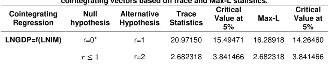
Table 2. Johansen maximum likelihood (ML) procedure: Test to determine the number of cointegrating vectors based on trace and Max-L statistics.

Cointegrating Regression

Null hypothesis

Alternative Hypothesis

Trace Statistics

Critical Value at

5%

Max-L

Critical Value at

5%

LNGDP=f(LNIM) r=0* r=1 20.97150 15.49471 16.28918 14.26460

r=2 2.682318 3.841466 2.682318 3.841466

Notes: a. * denotes rejection of null hypothesis at 5%.

b. Both Trace and Max-L statistics indicated one cointegrating equations at 5%

c. Critical values are obtained from (Mac Kinnon et al. 1999)

Trace and Max-L statistics and critical values are for the null hypothesis of at most r cointegration vectors and a linear trend. It is safe to conclude that there are two cointegrating vectors because both the Trace and Max-L statistics reject the null hypothesis of no cointegration vectors (r=0) and the null hypothesis of at least one cointegration vectors ( .

4.3. Granger Causality

The existence of cointegration implies that a causality exists between the two variables, however, it does not indicate the direction of the causal relationship, therefore, Granger causality has been tested for the short term and the long term. The lag length is selected by Akaike Information Criterion (AIC). Trials reported that AIC ranges between 6.85 (4 lags) and -3.75 (1 lag), thus, four lags have been used in estimating VECM.

Table 3. Granger causality results Source of causation

Short Run Long Run (ECT) Joint (Short-Run/ECT)

Dependent Variable

s Β1, Β1,

(t statistics) (F-Statistics)

- 5.47731* -0.5285 - 5.2729*

11.25756* - -1.2912 10.73587* -

Notes: a. The ECTs were derived by normalizing the cointegrating vector, resulting in r number of residuals. Figures beneath them are estimated t-statistics testing the null that they are each significant.

b. Short-run F-statistics are obtained from Wald test procedure with restrictions H_0: δ_(e,i)=0 in equation

γ and H_0: _(y,i)=0 in equation 4

c. The joint effect F-statistics are obtained from the Wald test procedure with restrictions H_0: δ_(e,i)=0 or

_1=0 in equation γ and H_0: _(y,i)=0 or _β=0 in equation 4.

d. * indicates significance at 5%

(9)

One may also want to check whether the two sources of causation are jointly significant or not. Testing the joint hypothesis for all iin equation 6 and

for all i in equation 7.

On analyzing the short-run causality, given the F-statistics on lagged variables, we can reject the null hypothesis of no Granger causality between imports and GDP. In other words, it may be concluded that there is a bi-directional Granger causality between imports and GDP since statistics in the F-statistics’ both equations are significant at 5%. In the short run, however, the coefficients on Error Correction Terms are not significant in both equations indicating that there is no Granger causality between imports and GDP. When considering the F-statistics of joint (strong) Granger causality we fail to reject the null hypothesis of no strong Granger causality in both equations. Therefore, we found a strong bi-directional Granger causality between imports and GDP.

5. Summary and Conclusion

This paper tried to reveal the causal relationship between imports and GDP for Turkey over the period 1998 Q1-2014 Q4 using a bivariate model of GDP and imports. The ADF test was used to test for unit root. It was found that both imports and GDP are non-stationary in their levels, but stationary in their first differences. Thus, it may be argued that these series are integrated of order one, denoted as I(1). The next step was to determine, if there are any, the number of cointegration vectors. Johansen maximum likelihood test was employed to find the number of cointegration vectors and the test detected one cointegration vector. On analyzing the Granger causality, given the results of ADF and Johansen tests, a VECM model was used rather than a VAR model; since the VAR model in such variables always carries the risk of spurious regressions.

The Granger causality was used to investigate the short-run, long-run and the joint causalities between imports and GDP. Results indicated a bi-directional Granger causality between these variables in the short run as well as the joint effect. The insignificance of t-statistics of Error Correction Terms in both equations indicated that there is no Granger causality from GDP to imports or from imports to GDP in the long run.

References

Aktas, C., β009. Türkiye’nin İhracat, İthalat ve Ekonomik Büyüme Arasındaki Nedensellik Analizi [Causality Analysis Between Exports Imports and Economic Development in Turkey]. Kocaeli Üniversitesi Sosyal Bilimler Enstitüsü Dergisi [Kocaeli University Journal of Social Sciences], 18(2), pp.35-47.

Bilgin, C., Sahbaz, A., β009. Türkiye’de Büyüme ve İhracat Arasındaki Nedensellik İlişkileri [Causality Relations Between Growth and Exports in Turkey]. Gaziantep Üniversitesi Sosyal Bilimler Dergisi [Gaziantep University Journal of Social Sciences], 8(1), pp.177-198.

CBRT, 2014. Ödemeler Dengesi Raporu 2014-II [Report of Balance of Payments 2014-II]. [online]. Available at http://www.tcmb.gov.tr/wps/wcm/connect/f07e0a7f-bb78-4c38-ac82c23c871fdc89/ODRapor_20142.pdf?MOD=AJPERES&CACHEID=ROOTWORKS PACEf07e0a7f-bb78-4c38-ac82-c23c871fdc89 (Accessed 22.02.2016).

Cetinkaya, M. and Erdogan, S., 2010. Var analysis of the relation between GDP, import and export: Turkey case. International Research Journal of Finance & Economics, 55, pp.135-152

Dickey, D. A. and Fuller, W. A., 1979. Distribution of the estimators for autoregressive time series with a unit root. Journal of the American Statistical Association, 74(366), pp.427-431. http://dx.doi.org/10.2307/2286348

Engle, R.F. and Granger, C.W.J., 1987. Co-integration and error correction: representation, estimation and testing. Econometrica, 55(2), pp.251-276.

(10)

Esfahani, H.S., 1991. Exports, imports, and economic growth in semi-industrialized countries. Journal of Development Economics, 35(1), pp.93-116. http://dx.doi.org/10.1016/0304-3878(91)90068-7

Gerni, C., Emsen, O.Ç., and Deger, M.K., 2008. İthalata dayalı ihracat ve ekonomik büyüme: 1980-2006 [Import Oriented Export and Economic Development 1980-2006]. [online]. İzmir: DEÜ İİBF İktisat Bölümü, β. Ulusal İktisat Kongresi [Izmir: DEU FEAS Department of Economics 2nd Economics Congress] Available at: <http://www.deu.edu.tr/userweb/iibf_kongre/dosyalar/deger.pdf> (Accessed 22.02.2016).

Ghatak, S., Milner, C., and Utkulu, U., 1997. Exports, export composition and growth: Cointegration and causality evidence for Malaysia. Applied Economics, 29(2), pp.213-223. http://dx.doi.org/10.1080/000368497327272

Granger, C.W.J. and Newbold, P., 1974. Spurious regressions in econometrics. Journal of Econometrics, 2, pp.111-120. http://dx.doi.org/10.1016/0304-4076(74)90034-7

Granger, C.W.J., 1969. Investigating causal relations by econometric models and cross-spectral methods, Econometrica, 37(3), pp.424-438. http://dx.doi.org/10.2307/1912791

Halicioglu, F., 2007. A multivariate causality analysis of export and growth for Turkey. [online]. Economics and Econometrics Research (MacKinnon, 1996) Institute (EERI), Brussels in EERI Research Paper Series, No. EERI_RP_2007_05. Available at: <http://www.eeri.eu/documents/wp/EERI_RP_2007_05.pdf> (Accessed 08.01.2016). Johansen, S. and Juselius, K., 1990. Maximum likelihood estimation and inference on

cointegration– with applications to the demand for money. Oxford Bulletin of Economics and Statistics, 52(2), pp.169–210. http://dx.doi.org/10.1111/j.1468-0084.1990.mp52002003.x

Mac Donald, J.M., 1994. Does import competition force efficient production? The Review of Economics and Statistics, 76(4), pp.721-727. http://dx.doi.org/10.2307/2109773

MacKinnon, J.G., 1996. Critical values for cointegration tests. Queen’s University Economics Department Working Paper, No. 1227, pp.1-19.

Mac Kinnon, J.G., Haug, A.A., and Michelis, L., 1999. Numerical distribution functions of likelihood ratio tests for cointegration. Journal of Applied Sciences, 14(5), pp.563-577. Masih, A. and Masih, R., 1998. A multivariate cointegrated modelling approach in testing

temporal causality between energy consumption, real income and prices with an application to two Asian LDCs, Applied Economics, 30(10), pp.1287-1298.

http://dx.doi.org/10.1080/000368498324904

Mehrara, M. and Firouzjaee, B.A., 2011. Granger causality relationship between export growth and GDP growth in developing countries: Panel cointegration approach. International Journal of Humanities and Social Science, 1(16), pp.223-231.

Ram, R., 1990. Import and economic growth: A cross country study. Economia Internazionale [International Economics], 43(1), pp.45-66.

Simsek, M., β00γ. İhracata dayalı-büyüme hipotezinin Türkiye ekonomisi verileri ile analizi, 1960-2002 [The Analysis of Export Led Hypothesis by Using Turkish Data]. Dokuz Eylül Üniversitesi İktisadi ve İdari Bilimler Fakültesi Dergisi [Dokuz Eylül University Journal of Faculty of Economics and Administrative Sciences], 18(2), pp.43-63.

Singh, J.P. and Konya, L., 2007. Causality between Indian exports, imports, and agricultural, manufacturing GDP. La Trobe University Working Paper series, No. 2007.02.