A New Method of Adaptive Integration with
Error Control for Bond-Based Peridynamics
Kebing Yu, X.J. Xin
∗, Kevin B. Lease
Abstract—Peridynamics is a new formulation of solid mechanics and possesses some advantages in handling discontinuities within a continuum. Since the formulation is based on direct interactions be-tween points in a continuum separated by a finite distance, integration of interactions between points plays a crucial role in peridynamics. This research is focused on developing a new method of numerical integration with error control for bond-based peridy-namics. In this method, the continuum is discretized into cubic cells, and integration over full and partial cells in the horizon of interaction are calculated ac-curately. An adaptive trapezoidal integration scheme with a combined relative-absolute error control is em-ployed. Numerical examples of areal force density for triaxial and pure shear loading show that the new method is much more accurate and efficient than the previous method published in the literature.
Keywords: peridynamics, adaptive error control, trape-zoidal integration
1
Introduction
Problems involving crack growth and damage are impor-tant in solid mechanics. The partial differential equations in the classic theory are incompatible with the disconti-nuities because the spatial derivatives needed by those equations are undefined along the crack tips or crack sur-faces. A non-local theory calledperidynamics has been developed by Silling in an attempt to overcome the afore-mentioned difficulty [1]. In peridynamics the classic par-tial differenpar-tial equations are replaced with integral equa-tions so that the same equaequa-tions hold true anywhere in the body, including crack tips or surfaces.
The peridynamic theory has been applied successfully to crack and damage problems [2,3]. A meshfree method to numerically implement the peridynamic theory was pro-posed in [4]. The peridynamic theory also serves as a nice framework that allows the use of other constitutive models [5–8]. The convergence of peridynamics has been studied in [9, 10]. The peridynamic theory has also been advanced from the original bond-based peridynamics to state-based peridynamics [11] which removes the restric-tion of a constant Poisson’s ratio of1
4 and introduces the
∗Department of Mechanical and Nuclear Engineering, Kansas
State University, Manhattan, KS 66506 USA Email: [email protected]
classic concepts of stress and strain. These new develop-ments also allow peridynamic theory to handle dynamic fracture problems [12, 13].
In the literature, the bond-based peridynamic theory has been focused mostly on dynamic material behavior rather than fundamental mechanics problems involving stress and strain calculations, and published methods of nu-merical integration [1, 4] yield poor stress results. In this work a new integration method is developed which allows for a more accurate integration of the governing equation in bond-based peridynamics. With this new method, the calculation of stresses and strains with predetermined ac-curacy can be achieved. The new method is verified with some well-defined elasticity problems with closed form solutions.
2
A Brief Review of Bond-Based
Peridy-namic Theory
Bond-based peridynamics [1, 4] assumes that the solid body is composed of small particles. Each particle in-teracts with others within a finite distance δ called the
horizon. The pairwise interaction between two particles exists even when they are not in contact. This physical interaction is referred to as a bond, which in some way has a close analogy to a mechanical spring.
In bond-based peridynamics, the equation of motion for particleiin the reference configuration at timet is:
ρu¨(xi, t) =
Hi
f[u(xj, t)−u(xi, t),xj−xi]dVj
+b(xi, t), ∀j ∈Hi (1)
whereHiis a spherical neighborhood of particles that
in-teracts with particlei,dVjis an infinitesimal volume asso-ciated with particlej,uis the displacement vector field, bis a prescribed body force density field,ρ is the mass density, and f is the pairwise peridynamic force (hence-forth referred to as thebond force) function whose value is the force vector (per unit volume squared) that particle
jexerts on particlei.
There are two frequently used terms in peridynamic the-ory: therelative position ξof two particlesiandj in the reference configuration:
terial is called thePrototype Microelastic Brittle (PMB) material [4]. For a PMB material, the bond force func-tionf is a linear function of the current bond stretchs, which also serves as the constitutive model:
f(η,ξ) =μ(ξ)18K
πδ4
η+ξ
|η+ξ|s (4) whereK is the bulk modulus, andsis defined as:
s=|η+ξ| − |ξ|
|ξ| (5)
and μ(ξ) is a history-dependent scalar-valued function that equals either 1 or 0:
μ(ξ) =
1 for s < s0
0 otherwise (6)
wheres0 is the critical bond stretch for bond failure.
The bond-based peridynamic theory can be related to classic elasticity theory through the concept of force per unit area. Assume an infinite bodyRundergoes a
defor-mation. Choose a particlexand a unit vectornatxand let a plane pass throughxto divide the whole body into two parts: R− andR+:
R+={x′∈R: (x′−x)·n≥0} (7)
R−={x′∈R: (x′−x)·n≤0} (8)
and letL be the following set of colinear points:
L ={ˆx∈R−:ˆx=x−pn,0≤p <∞} (9)
Theareal force density τ(x,n) at x in the direction of unit vectornis defined as [1]:
τ(x,n) =
L
R+
f(u′−ˆu,x′−ˆx)dV
x′dˆl (10)
wheredˆl represents the differential path length overL.
A meaningful representation of a stress tensorσ can be proposed [1]:
τ(x,n) =σn, ∀n (11)
This stress tensor is a Piola-Kirchhoff stress tensor since τ(x,n) is force per unit area in the reference configura-tion.
In the literature, a meshfree code named EMU [4] has been developed to numerically implement the peridy-namic theory. In this implementation the domain of in-terest is discretized into a cubic lattice system. Each
source node. Based on the peridynamic theory, the fam-ily nodes of a source node is a set of nodes which have peridynamic interaction with the source node. Following the concept of horizon, the family nodes form a spheri-cal neighborhood (henceforth referred to as the horizon sphere) centered at the source node with radius equals to horizon. A horizon of three times the grid spacing has been suggested in [4].
For numerical integration, the equation of motion at the source nodeican be discretized to:
ρu¨i=
j
f(η,ξ)dVj+bi, ∀j∈Hi (12)
whereHiis the horizon sphere of nodei. For each family
nodej in Hi, the integration is carried out over the cell
volume of nodej which may be fully or partially in the horizon sphere. Equation (12) is the discretized form of equation of motion corresponding to Eqn. (1).
Because the principle of bond-based peridynamics in-volves only two-particle interactions, it is inevitable that all bond-based peridynamic materials have a fixed Pois-son’s ratio of 1
4 [1]. A further development of the theory
removes this restriction [11].
3
Deficiencies in the Existing Numerical
Implementation of Peridynamics
There are two deficiencies in the existing implementation of peridynamics presented in [1, 2, 4] that may prevent it from achieving accurate and consistent results:
Figure 1: (A) Accounting of the family nodes by the numerical implementation presented in [2, 4]; (B) The volume of the quarter horizon sphere calculated by the cubic-cell integration.
(2) The three-dimensional integration in Eqn. (12) is performed using a one-point integration [2, 4, 14]:
ρu¨i =
j
f(η,ξ)·β(∆x)3
+bi (13)
where (∆x)3 is the cell volume and β is thevolume
re-duction factor defined as:
β= ⎧ ⎪ ⎨
⎪ ⎩
1 for |ξ| ≤δ−0.5∆x δ+ 0.5∆x− |ξ|
∆x for |ξ| ≤δ+ 0.5∆x
0 otherwise
(14)
For convenience, the integration method implemented in [1, 2, 4] is referred to as cubic-cell integration. Fig-ure 1B illustrates the cubic-cell integration method when |ξ|is within the range ofδ-0.5∆xandδ+0.5∆x,i.e., the cubic cell is partially in the horizon sphere. In the figure, the circular arc represents a quarter of the horizon sphere. The volume of the quarter sphere calculated by the cubic-cell integration is marked as the dark shaded area. The volume missed in the calculation is marked as the hor-izontal line patterned area. For family node 1, a small extra volume is added to the actual intersection volume. For family node 2, the cubic-cell integration overcompen-sates the missing volume in the cell with the calculated volume (vertical slashed area). For node 3, since it is not counted as a family node, its cell contributes nothing to the integration. Partial cell volumes of three other nodes (represented by unnumbered open dots) in the figure are also excluded from the calculation. Such an approxima-tion in counting the volume integraapproxima-tion elements leads to poor accuracy of the numerical bond-based peridynamic model.
4
A New Method of Adaptive
Integra-tion with Error Control
The key to improving the accuracy in the numerical im-plementation of peridynamics is to evaluate the integra-tion in Eqn. (12) properly. Kilicet al [7] recently intro-duced a volume integration scheme based on the collo-cation method. In this scheme, the Gaussian integration
Figure 2: Modified accounting of family nodes (solid dots) by the adaptive integration.
method with shape function transformation [8] is used to solve the volume integration over every subdomain. The work presented here employs an adaptive integra-tion with error control. This method bears some resem-blance to the recent advances on XFEM method in that both identify the intersection configurations of cutter in-terfaces/elements and cut elements [15–17].
The new integration method proposed here is focused on a more accurate numerical integration of Eqn. (12),i.e., the integration is calculated over the intersection volume with controlled accuracy. For convenience, the new inte-gration method is referred to asadaptive integration.
4.1
Modification of Counting the Family
Nodes
To integrate Eqn. (12) accurately, the family nodes must be counted properly. Besides all the nodes fully in the horizon sphere, the adaptive integration also considers those nodes which areout of the horizon sphere yet with cell volumes intersecting the horizon sphere as family nodes. For every node, the shortest distance from the source node to the cell associated with that node is cal-culated. If the distance is smaller than the horizon, then the cell has volume inside the horizon sphere and the node is considered a family node. The newly-evaluated family nodes are shown in Fig. 2.
4.2
Categorization of Geometric
Configura-tions
The integration limits in three directions need to be de-termined to evaluate the integral in Eqn. (12). For cells fully inside the horizon sphere the integration limits in the X (Y, or Z) direction are simply the coordinates of projection of the two opposite cell walls normal to X (Y, or Z) onto the X (Y, or Z) axis. For cells partially in-side the horizon sphere, the limits are more difficult to calculated and are described in detail below. Two terms are defined: family coordinate is referred to as the local coordinate centered at the source node, andfirst octant
Figure 3: Possible geometric configurations for three sub-types of type one. (A) Subtype 1; (B) Subtype 2; (C) Subtype 3.
4.2.1 Geometric Configuration Type One
This type is for the configuration whenthe family node is located on one axis of the family coordinate. Without loss of generality, assume nodej is in the first octant of the global coordinate system and on the Z+ axis of the family coordinate. If the global coordinates of the source node i and family node j are given as (xi
1, xi2, xi3) and
(xj1, xj2, xj3) respectively, then with the given assumption,
xi
1=x
j
1, xi2=x
j
2.
There are three subtypes of possible configurations be-tween nodeiandj. Figure 3 depicts one possible geomet-ric configuration for each subtype. Subtype 1 is chosen to illustrate the sequence of finding the integration limits. As shown in Fig. 3A, the intersection volume is formed by vertices A-B-C-D-E. The integration is carried out by integrating the Z direction first and the X direction last. The equation of circleA-B-C-D and the X coor-dinates of points B and D need to be solved to define the integration limits of X and Y directions. After they are solved, the integration of Eqn. (12) for the geometric configuration shown in Fig. 3A is expressed as:
I= xD1
xB 1
xi2+
√
δ2
−(xj3−xi3−0.5∆x) 2
−(X−xi 1)
2
xi 2−
√
δ2
−(xj3−xi3−0.5∆x)2−(X−xi1)2
× xi3+
√
δ2 −(X−xi
1) 2
−(Y−xi 2)
2
xj 3−0.5∆x
f(η,ξ)dxdydz (15)
wheredxdydzis the infinitesimal volume associated with the integration point within the intersection volume.
4.2.2 Geometric Configuration Type Two
This type is for the configuration whenthe family node is not located on any axis of the family coordinate. Fig-ure 4 shows one possible configuration for this type. The intersection volume is formed by vertices A-B-C-D-E
-F-G-K-L. Based on the figure, the integration can be
Figure 4: One possible geometric configuration for type two. (A) 3D view; (B) Projection onto the front face of the cell.
divided into two parts: part 1 integrates over the vol-ume formed by verticesA-B-C-D-E-F-G-F′-E′-L, part
2 integrates over the volume formed by verticesF-E-M
-F′-E′-K. After all the integration limits are solved, the
integration can be carried out readily.
4.3
Adaptive Integration Using the
Trape-zoidal Rule with Error Control
Because of its simplicity and ease of error control, the composite trapezoidal rule [18] is used to carry out the preceding integrations. For the 1D case, it is stated as:
b
a
f(x)dx≈b−na
×
f(a) +f(b)
2 +
n−1
k=1
f
a+kb−a n
(16)
where the integernis referred to as thetrapezoidal index. The composite trapezoidal rule is used to achieve piece-wise approximation of the curved surface of the intersec-tion volume. The accuracy can be easily improved by adding more trapezoidal points into the calculation, i.e., by increasing the value ofn. By applying the composite trapezoidal rule to each direction of the aforementioned 3D integrations (such as Eqn. (15)), the position of the integration points can be found.
A combined relative-absolute error control is used to achieve the prescribed accuracy. If the value of integra-tion from the current iteraintegra-tion is denoted asIrwhereris the current step, and the value from the previous itera-tion is denoted asIr−1, the error control scheme is stated
as the following pseudo code: if (abs(Ir−1)> T OL)
if (abs(Ir−Ir−1)<=EP S·abs(Ir−1))
returnIr
else
if (abs(Ir−Ir−1)<=EP S)
returnIr
Figure 5: The convergence rates of the horizon sphere volume calculation by two integration methods.
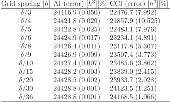
Table 1: The volume of horizon sphere calculated by two volume integration methods.
Grid spacing [h] AI (error) [h3][%] CCI (error) [h3][%]
δ/3 24416.9 (0.050) 22476.7 (7.992)
δ/4 24421.8 (0.029) 21857.9 (10.525)
δ/5 24422.8 (0.025) 22483.1 (7.976)
δ/6 24424.9 (0.017) 23234.1 (4.891)
δ/8 24426.4 (0.011) 23117.8 (5.367)
δ/9 24426.9 (0.009) 23507.4 (3.773)
δ/10 24427.4 (0.007) 23485.6 (3.862)
δ/15 24428.2 (0.003) 23839.0 (2.415)
δ/20 24428.5 (0.002) 23933.7 (2.028)
δ/30 24428.8 (0.001) 24123.5 (1.251)
δ/36 24428.8 (0.001) 24168.5 (1.066)
The adaptive integration scheme developed in this work can evaluate an integration with controlled accuracy. The convergence speed is proved to be close to quadratic (i.e.,
O(∆x2)) and the error control method is quite effective.
5
Numerical Results
5.1
The Volume of the Horizon Sphere
In this example, the adaptive integration (AI) and cubic-cell integration (CCI) are used to calculate the volume of the horizon sphere of a source node. As only a finite array of nodes is used in the simulation, the source node is chosen at or near the center of the array so that its horizon sphere is fully inside the array. For example, in a uniform grid with ∆x=δ/3 as shown in Fig. 2, nodei
is the source node which has a total of 250 family nodes. Various grid spacings with a fixed horizon are used to investigate the rate of convergence, defined as the slope of the relative error-grid spacing plot, for both methods.
The physical length unit is denoted as h in the follow-ing calculations. The horizon is fixed to 18h so that the accurate volume of the horizon sphere is 4πR3/3 (or
24429.0h3). Table 1 compares the results by the AI and
CCI methods with grid spacing ranging from ∆x=δ/3 to ∆x=δ/36. The rates of convergence for the two methods are shown in Fig. 5. Both methods become more
accu-Figure 6: The convergence rates of σ33 in triaxial stress
state andσ13in pure shear for two integration methods.
rate as the grid gets finer. The results by the AI method match the accurate volume very well (within 0.05%) even at the coarsest grid (∆x=δ/3) and maintain a conver-gence rate of 1.73. For a given grid spacing ∆x, the AI method is 2 to 3 orders of magnitude more accurate than the CCI method. Obvious fluctuations during the grid refinement (at ∆x = δ/4 and ∆x = δ/8) are observed from the results by the CCI method, which is possibly caused by the deficiencies discussed in Section 3.
5.2
Infinite Body Under Two Stress States
In this example, the areal force densities at a source node under triaxial (σ11=100N/h2, σ22=−150N/h2,
σ33=220N/h2) and pure shear (σ13=200N/h2) stress
states for an infinite body are calculated by both the AI and CCI methods and are compared with the closed form solutions. Various grid spacings with a fixed horizon are used to investigate the rate of convergence for both methods.
For example, for a grid spacing of ∆x = δ/3, a uni-form gird of 10×10×10 nodes is created and the node near the center of the domain at the coordinate of (∆x/2,∆x/2, ∆x/2) is chosen to be the source node. The displacement of every node is prescribed according to the displacement solution of an infinite body for the given stress state. Consequently, this finite domain behaves like an infinite body. By assuming small deformation and lin-ear elastic response, the closed form solution for stress at every node can be solved using classic elasticity theory.
A PMB material with Young’s modulus of 1.0×10⁵N/h2
is used. The horizon is fixed at 18hfor all the calcula-tions. For the AI method, the tolerance TOL is chosen to be 1.0×10⁻⁴. The areal force density at the source
node is calculated based on Eqn. (10).
The convergence rates of the largest principle stressσ33
6
Conclusions
Integration plays an important role in the formulation of peridynamics. Published cubic-cell integration method in the literature, however, gives relatively low accuracy and the convergence rate with mesh refinement is low, in the range of 0.66 to 1.04 for the examples tested. The study here presents a new adaptive integration method with er-ror control. The adaptive integration method improves the numerical implementation of bond-based peridynam-ics in the following ways:
1. The way to count the family nodes is modified to include all the material points in the whole horizon sphere.
2. A systematic categorization of geometric configura-tion for the intersecconfigura-tion volume between the cell of a family node and the horizon sphere of the source node is developed so that accurate integration over the intersection volume becomes possible.
3. Adaptive trapezoidal quadrature with a combined relative-absolute error control is introduced into the new integration method for achieving numerical in-tegration with desired accuracy.
4. Examples show results produced by the new adaptive integration method match the closed form solutions quite well even at the coarsest grid. The tested ex-amples show the new adaptive integration method has high convergence rates (in the range of 1.53 to 1.72, or nearly quadratic, for the examples tested) and is both accurate and efficient.
References
[1] Silling, S.A., “Reformulation of Elasticity Theory for Discontinuities and Long-Range Forces,” J. Mech. Phys. Solids, V48, N1, pp.175–209, 1/00.
[2] Silling, S.A., Askari, E., “Peridynamic Modeling of Impact Damage,” 2004 ASME/JSME Pressure Ves-sels and Piping Conf, San Diego, USA, pp.197–205, 7/04.
[3] Xu, J., Askari, A., Weckner, O., Silling, S.A., “Peri-dynamic Analysis of Impact Damage in Composite Laminates,” J. Aerosp. Eng., V21, N3, pp.187–194, 7/08.
[4] Silling, S.A., Askari, E., “A Meshfree Method Based on the Peridynamic Model of Solid Mechanics,”
Comput. Struct., V83, N17, pp.1526–1535, 6/05.
[7] Kilic, B., Madenci, E., “Structural Stability and Failure Analysis Using Peridynamic Theory,”Int. J. Non-Linear Mech., V44, N8, pp.845–854, 10/09.
[8] Kilic, B., Agwai, A., Madenci, E., “Peridy-namic Theory for Progressive Damage Prediction in Center-cracked Composite Laminates,” Compos. Struct., V90, N2, pp.141–151, 9/09.
[9] Silling, S.A., Lehoucq, R.B., “Convergence of Peri-dynamics to Classical Elasticity Theory,” J. Elast., V93, N1, pp.13–37, 10/08.
[10] Bobaru, F., Yang, M., Alves, L.F., Silling, S.A., Askari, E., Xu, J., “Convergence, Adaptive Refine-ment, and Scaling in 1D Peridynamics,”Int. J. Nu-mer. Methods Eng., V77, N6, pp.852–877, 2/09.
[11] Silling, S.A., Epton, M., Weckner, O., Xu, J., Askari, E., “Peridynamic States and Constitutive Model-ing,”J. Elast., V88, N2, pp.151–184, 8/07.
[12] Foster, J.T., Silling, S.A., Chen, W.W., “State Based Peridynamic Modeling of Dynamic Fracture,” SEM Annual Conf and Exposition on Experimen-tal and Applied Mechanics, Albuquerque, USA, pp.2312–2317, 6/09.
[13] Warren, T.L., Silling, S.A., Askari, A., Weckner, O., Epton, M.A., Xu, J., “A Non-ordinary State-based Peridynamic Method to Model Solid Material Defor-mation and Fracture,”Int. J. Solid. Struc., V46, N5, pp.1186–1195, 3/09.
[14] EMU Website, http://www.sandia.gov/emu/emu.htm.
[15] Fries, T.P., “A Corrected XFEM Approximation Without Problems in Blending Element,”Int. J. Nu-mer. Methods Eng., V75, N5, pp.503–532, 7/08.
[16] Tabarraei, A., Sukumar, N., “Extended Finite Ele-ment Method on Polygonal and Quadtree Meshes,”
Comput. Meth. Appl. Mech. Eng., V197, N5, pp.425– 438, 1/08.
[17] Mayer, U.M., Gerstenberger, A., Wall, A.W., “Interface Handling for Three-dimensional Higher-order XFEM-computations in Fluid-structure Inter-action,” Int. J. Numer. Methods Eng., V79, N7, pp.846–869, 8/09.
![Figure 1: (A) Accounting of the family nodes by the numerical implementation presented in [2, 4]; (B) The volume of the quarter horizon sphere calculated by the cubic-cell integration.](https://thumb-eu.123doks.com/thumbv2/123dok_br/17097832.237221/3.892.111.380.72.223/figure-accounting-numerical-implementation-presented-horizon-calculated-integration.webp)