Estimates of global terrestrial isoprene emissions using MEGAN (Model of Emissions of Gases and Aerosols from Nature)

(1)

ACPD

6, 107–173, 2006

MEGAN estimates of global isoprene

emissions

A. Guenther et al.

Title Page

Abstract Introduction

Conclusions References

Tables Figures

◭ ◮

Back Close

Full Screen / Esc

Print Version

Interactive Discussion

EGU

Atmos. Chem. Phys. Discuss., 6, 107–173, 2006 www.atmos-chem-phys.org/acpd/6/107/

SRef-ID: 1680-7375/acpd/2006-6-107 European Geosciences Union

Atmospheric Chemistry and Physics Discussions

Estimates of global terrestrial isoprene

emissions using MEGAN (Model of

Emissions of Gases and Aerosols from

Nature)

A. Guenther1, T. Karl1, P. Harley1, C. Wiedinmyer1, P. I. Palmer2, and C. Geron3 1

Atmospheric Chemistry Division, National Center for Atmospheric Research, 1850 Table Mesa Drive, Boulder Colorado 80305, USA

2

School of Earth and Environment, University of Leeds, Leeds, LS2 9JT, UK

3

National Risk Management Research Laboratory, U.S. Environmental Protection Agency, 109 TW Alexander Dr., Research Triangle Park, NC 27711, USA

Received: 16 November 2005 – Accepted: 30 November 2005 – Published: 3 January 2006 Correspondence to: A. Guenther (guenther@ucar.edu)

(2)

ACPD

6, 107–173, 2006

emissions

A. Guenther et al.

Title Page

Tables Figures

◭ ◮

Back Close

Full Screen / Esc

Print Version

EGU

Abstract

Reactive gases and aerosols are produced by terrestrial ecosystems, processed within plant canopies, and can then be emitted into the above-canopy atmosphere. Estimates of the above-canopy fluxes are needed for quantitative earth system studies and as-sessments of past, present and future air quality and climate. The Model of Emissions 5

of Gases and Aerosols from Nature (MEGAN) is described and used to quantify net terrestrial biosphere emission of isoprene into the atmosphere. MEGAN is designed for both global and regional emission modeling and has global coverage with∼1 km2 spatial resolution. Field and laboratory investigations of the processes controlling iso-prene emission are described and data available for model development and evalu-10

ation are summarized. The factors controlling isoprene emissions include biological, physical and chemical driving variables. MEGAN driving variables are derived from models and satellite and ground observations. Broadleaf trees, mostly in the tropics, contribute about half of the estimated global annual isoprene emission due to their rel-atively high emission factors and because they are often exposed to conditions that 15

are conducive for isoprene emission. The remaining flux is primarily from shrubs which are widespread and dominate at higher latitudes. MEGAN estimates global annual iso-prene emissions of ∼600 Tg isoprene but the results are very sensitive to the driving variables, including temperature, solar radiation, Leaf Area Index, and plant functional type. The annual global emission estimated with MEGAN ranges from about 500 to 20

750 Tg isoprene depending on the driving variables that are used. Differences in es-timated emissions are more than a factor of 3 for specific times and locations. It is di_fficult to evaluate isoprene emission estimates using the concentration distributions simulated using chemistry and transport models due to the substantial uncertainties in other model components. However, comparison with isoprene emissions estimated 25

(3)

ACPD

6, 107–173, 2006

emissions

A. Guenther et al.

Title Page

Tables Figures

◭ ◮

Back Close

Full Screen / Esc

Print Version

EGU

simulated by global climate models for year 2100, MEGAN estimates that isoprene emissions increase by more than a factor of two. This is considerably greater than pre-vious estimates and additional observations are needed to evaluate and improve the methods used to predict future isoprene emissions.

1. Introduction

5

Chemicals produced by the biosphere include volatile compounds that are emitted into the air where they can have a substantial impact on the chemistry of the atmosphere. These compounds are dominated by volatile organic compounds (VOCs) both in total mass and number of compounds. The impact of biogenic VOCs on global chemistry and climate has been investigated using global models (e.g., Houweling et al., 1998; 10

Guenther et al., 1999a; Granier et al., 2000; Poisson et al., 2000; Collins et al., 2002; Sanderson et al., 2003) while regional air quality models have included biogenic VOC emissions in efforts to develop pollution control strategies (e.g., Pierce et al., 1998). Biogenic VOC emissions were included as inputs to regulatory regional oxidant mod-els in the mid 1980s (Pierce and Waldruff, 1991) and by the 1990s were routinely 15

included in chemical transport models, but typically as off-line, static emission inven-tories. There is increasing demand for biogenic emission algorithms that can be inte-grated into regional and global models. This would facilitate studies of chemical and physical feedbacks to biogenic emissions and other earth system components and to ensure consistency in the landcover and weather variables.

20

Although hundreds of biogenic VOC have been identified, two compounds dominate the annual global flux to the atmosphere: methane and isoprene. Microbes are the ma-jor source of biogenic methane, while over 90% of all isoprene is emitted from terrestrial plant foliage. Minor sources of isoprene include microbes, animals (including humans) and aquatic organisms (Wagner et al., 1999). Methane and isoprene each comprises 25

(4)

ACPD

6, 107–173, 2006

emissions

A. Guenther et al.

Title Page

Tables Figures

◭ ◮

Back Close

Full Screen / Esc

Print Version

EGU

long-lived (years) compound with a well mixed distribution throughout the atmosphere while isoprene is short-lived (minutes to hours) with atmospheric concentrations that vary several orders of magnitude over a time scale of less than one day and over spa-tial scales of less than a few km. As a result, we can be relatively certain of the annual global emission of methane, based on estimates of the global atmospheric burden and 5

the average lifetime; however, the annual global isoprene emission is much less well constrained. Satellite-derived global distributions of isoprene oxidation products (e.g., formaldehyde and carbon monoxide) are beginning to provide constraints on global isoprene emission rates but they too are associated with significant uncertainties and they cannot provide estimates of past (pre-satellite era) and future emissions. There 10

remains a need for models that can estimate past, current and future isoprene emis-sions.

In the early 1990s, the International Global Atmospheric Chemistry (IGAC) Global Emissions Inventory Activity (GEIA) initiated working groups to develop global emission inventories on a 1 degree by 1 degree grid for use in global chemistry and transport 15

models (Graedel et al., 1993). The IGAC-GEIA natural VOC working group developed a model of emissions of isoprene and other VOC (Guenther et al., 1995). A regional biogenic emission model, the Biogenic Emissions Inventory System or BEIS (Pierce and Waldruff, 1991), was developed in the mid 1980s and replaced by a second gener-ation model, BEIS2 (Pierce et al., 1998), in the mid 1990s. This manuscript describes 20

the Model of Emissions of Gases and Aerosols from Nature (MEGAN) which was de-veloped to replace both the Guenther et al. (1995) global emission model and the BEIS/BEIS2/BEIS3 regional emission models. We focus in this paper on isoprene emissions and will describe MEGAN procedures for simulating emissions of other gases and aerosols elsewhere. Field and laboratory investigations of the processes 25

(5)

iso-ACPD

6, 107–173, 2006

emissions

A. Guenther et al.

Title Page

Tables Figures

◭ ◮

Back Close

Full Screen / Esc

Print Version

EGU

prene emissions to earth system changes (e.g., climate, chemistry and landcover) are presented and used to identify major uncertainties.

2. Isoprene observations

Enclosure methods were first used to study biogenic VOC emissions in the late 1920s (Isidorov, 1990). In the following 75 years, investigators enclosed thousands of leaves, 5

branches and whole plants in bags, jars, and cuvettes to characterize fluxes of isoprene and other VOCs. The earliest studies focused on monoterpenes (see Went, 1960; Isidorov, 1990) but the co-discovery of abundant emissions of isoprene from some plant species by Rasmussen and Went (1965) in the U.S. and Sanadze (1957) in the former Soviet Union led to considerable interest in emissions of this compound. Wiedinmyer et 10

al. (2004) reviewed the scientific literature describing enclosure measurements of foliar emissions of isoprene and other biogenic VOC (BVOC) and have compiled this informa-tion into an online searchable database (seehttp://bvoc.acd.ucar.edu). The database includes the results of more than 160 studies that have characterized isoprene emis-sions from hundreds of plant species using enclosure measurement systems.

15

Rasmussen and Went (1965) extrapolated a few biogenic VOC enclosure observa-tions to the global scale by simply multiplying a typical emission rate by the global area covered by vegetation and the fraction of the year that plants are growing. The resulting annual total (isoprene plus all other non-methane biogenic VOC) flux esti-mate of 438 Tg (1012g) is about a factor of three lower than the estimate of Guenther 20

et al. (1995). A simple approach like this can be used to establish an upper bound global isoprene emission estimate. The highest leaf-level isoprene emission rates are ∼150µg g−1h−1. If all leaves emitted continuously at this rate, the global annual iso-prene emission would exceed 25 Gt (1015g). However, the actual global annual iso-prene emission is about 2% of this rate due to environmental conditions that are not 25

(6)

ACPD

6, 107–173, 2006

emissions

A. Guenther et al.

Title Page

Tables Figures

◭ ◮

Back Close

Full Screen / Esc

Print Version

EGU

Guenther et al. (1995) relied primarily on enclosure measurement studies to assign leaf level isoprene emission factors to 72 global ecosystems. The emission factors for about half of these ecosystems were assigned based on observations reported in twenty publications and the remaining ecosystems were assigned default values. Only three of the twenty publications included studies from tropical regions even though the 5

tropics were estimated to contribute about 80% of the global annual isoprene emis-sions. Furthermore, the emission activity algorithms that describe the response of isoprene to temperature and light were based on investigations of temperate plants growing in temperate weather conditions and had not been evaluated by any measure-ments in the tropics.

10

Thousands of isoprene emission rate measurements have been made using enclo-sure techniques in the decade since the Guenther et al. (1995) model was developed. Many of these measurements have been incorporated into the isoprene emission fac-tors used for MEGAN. Recent studies have also shown that much of the observed isoprene variability among plant species with significant emission rates (e.g.,Quercus,

15

Liquidambar, Nyssa, Populus, Salix, andRobiniaspecies) can be attributed to weather, plant physiology and the location of a leaf within the canopy rather than genetics (Geron et al., 2000). Other studies have characterized how emissions respond to various fac-tors including leaf age (Monson et al., 1994; Petron et al., 2001), nutrient availability (Harley et al., 1994), weather (Sharkey et al., 2000) and the chemical composition of 20

the atmosphere (Velikova et al., 2005; Rosentiel et al., 2003). Of particular impor-tance for global modeling, many more enclosure measurements have been conducted in tropical landscapes (Keller and Lerdau, 1999; Guenther et al., 1999a; Kesselmeier et al., 2000; Klinger et al., 2002; Kuhn et al., 2002; Harley et al., 2004). Accompanying these emission measurements have been efforts to process tree inventory data into a 25

format suitable for characterizing regional isoprene emission distributions.

(7)

under-ACPD

6, 107–173, 2006

emissions

A. Guenther et al.

Title Page

Tables Figures

◭ ◮

Back Close

Full Screen / Esc

Print Version

EGU

standing of chemical sinks and deposition losses within vegetation canopies, 2) artifi-cially disturbed emission rates due to the enclosure, 3) di_fferences between the func-tioning of individual ecosystem components (e.g. leaves) and the entire ecosystem, and 4) limited sample size within the enclosure (relative to the whole landscape), as well as uncertainties associated with canopy microclimate models themselves. Direct 5

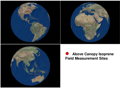
measurements of above canopy fluxes are suitable for characterizing whole canopy net emission rates and are fortunately becoming increasingly available to parameterize key global ecosystems. Above canopy isoprene flux measurement systems continue to be-come more reliable and widespread than in the past. Isoprene fluxes can now be mea-sured routinely using eddy flux techniques such as relaxed eddy accumulation (e.g., 10

Guenther et al., 1996) and eddy covariance (Guenther and Hills, 1998). In addition to these direct flux measurement methods, inverse modeling and gradient approaches use isoprene concentrations obtained from aircraft and tethered balloon sampling plat-forms to characterize isoprene emissions across spatial scales of tens to hundreds of km2 (e.g., Greenberg et al., 1999). The geographical distribution of the >80 studies 15

used to assign the isoprene emission factor distributions described in this manuscript is illustrated in Fig. 1. More than 80 laboratory studies were also incorporated into the development of model algorithms and emission factors.

3. MEGAN model description

MEGAN estimates the net emission rate (mg compound m−2 _{earth surface h}−1_{) of}

20

isoprene and other trace gases and aerosols from terrestrial ecosystems into the at-mosphere at a specific location and time as

Emission=ε·γ·ρ (1)

(8)

ACPD

6, 107–173, 2006

emissions

A. Guenther et al.

Title Page

Tables Figures

◭ ◮

Back Close

Full Screen / Esc

Print Version

EGU

activity factor that accounts for emission changes due to deviations from standard con-ditions andρ (normalized ratio) is a factor that accounts for chemical production and loss within plant canopies. The MEGAN canopy-scale emission factor differs from most other biogenic emission models which use a leaf-scale emission factor. The standard conditions for landcover characteristics include a leaf area index, LAI, of 5 and a canopy 5

with 92% mature leaves; current environmental conditions include a solar angle (de-grees from horizon to sun) of 60 de(de-grees, a photosynthetic photon flux density (PPFD) transmission (ratio of PPFD at the top of the canopy to PPFD at the top of the atmo-sphere) of 0.6, air temperature=303 K, humidity=14 g kg−1, wind speed=3 m s−1, and soil moisture=0.3 m3m−3; average canopy environmental conditions of the past 24 to 10

240 h include leaf temperature₌297 K and PPFD₌200µmol m−2_s−1_{for sun leaves and}

50µmol m−2s−1for shade leaves. The factorγ is equal to unity at these standard con-ditions. Note that a solar angle of 60 degrees and a PPFD transmission of 0.6 results in a PPFD of∼1500µmol m−2s−1. Emissions are calculated separately for each plant functional type (PFT) that occurs within a grid cell. The emission from each PFT is 15

summed to estimate the total emission. MEGAN is a global scale model with a base resolution of∼1 km2 (30 s latitude by 30 s longitude) enabling both regional scale and global scale simulations. The MEGAN emission factors, algorithms and driving vari-ables can be accessed through a public data portal (see http://bai.acd.ucar.edu) at the base and lower resolutions for specific years. Methods for estimating each of the 20

factors in Eq. (1) are described in the following sections.

3.1. Emission factor,ε

Isoprene is emitted by soil bacteria, algae, and in the breath of animals (including hu-mans) as well as plants (Wagner et al., 1999). Only vegetation emissions have been shown to occur at levels that can influence atmospheric composition although rela-25

tively little is known about soil bacteria. The isoprene emission rates of different plant species range from<0.1 to >100µg g−1_h−1_{. Very low and very high emitters often}

(9)

ACPD

6, 107–173, 2006

emissions

A. Guenther et al.

Title Page

Tables Figures

◭ ◮

Back Close

Full Screen / Esc

Print Version

EGU

including Quercus (oaks), Picea (spruce), Abies (firs) and Acacia. The large taxo-nomic variability makes the characterization of isoprene emission factor distributions a challenging task. The MEGAN landcover approach divides each grid cell into vege-tated and non-vegevege-tated earth surface, and places all vegetation into one of six PFTs. These include three tree categories (broadleaf, fineleaf evergreen and fineleaf decid-5

uous), categories for shrubs and crops, and a category for all other vegetation (i.e., grasses, sedges, forbs, and mosses). In contrast to the ecosystem approach, in which each location or model grid cell is characterized by a single ecosystem type, the PFT approach covers each grid cell with a variable fraction of each PFT. MEGAN accounts for regionalεvariations using geographically gridded databases of isoprene emission 10

factors for each PFT. A unique isoprene emission factor for a given PFT, for example, broadleaf trees, can be assigned to each grid cell, depending on the measured or as-sumed isoprene emission characteristics of the broadleaf tree species found in that cell.

Table 1 illustrates the differences in the global average isoprene emission factors for 15

the six PFTs. Broadleaf trees and shrubs have the highest average emission factor. The average fineleaf evergreen tree isoprene emission factor is∼84% lower than the average broadleaf tree emission factor. The fineleaf deciduous tree and grass/other PFTs have average emission factors that are about a factor of 20 lower than the av-erage broadleaf tree emission factor, while the crop isoprene emission factor is about 20

two orders of magnitude lower. The substantial differences in these global average iso-prene emission factors demonstrates the value of the PFT approach but Table 1 also shows that there is considerable variability associated with the isoprene emission fac-tors assigned to a PFT. For example, the isoprene emission factor for broadleaf trees ranges from 0.1 to 30 mg m−2h−1. Global total isoprene emissions can be approxi-25

(10)

ACPD

6, 107–173, 2006

emissions

A. Guenther et al.

Title Page

Tables Figures

◭ ◮

Back Close

Full Screen / Esc

Print Version

EGU

substantial errors in estimates for any location whereεdeviates significantly from the PFT averageε.

Isoprene emission factor distributions for each PFT were estimated by combining the isoprene observations described in Sect. 2 with landcover information that includes ground measurement inventories, satellite based inventories, and ecoregion descrip-5

tions. The available landcover and isoprene observations differ considerably for the 6 PFTs and also differ for geographic regions. In some cases, vegetation inventories were combined with satellite observations to generate high resolution (∼1 km2) species composition distributions, while in other cases general descriptions were used to char-acterize global ecoregions. A description of the methods used for each PFT is given 10

below.

Since geographical distributions of PFTs and PFT-specific isoprene emission factors change with time, the distributions used to estimate emissions should be representative of the time period being simulated. Climate-driven changes in species composition can substantially modify both PFT and εvalues on a time scale of decades to centuries 15

(e.g., Turner et al., 1991; Martin and Guenther, 1995) while changes associated with land management can occur on time scales of years (e.g., Guenther et al., 1999b; Schaab et al., 2000). Global PFT andεdatabases are needed on time scales of 50 to 100 years for simulating global earth system changes. A considerably shorter time step for PFT andεinputs is required for regional studies investigating the impacts of 20

land cover change.

3.1.1. Trees

Trees have been the focus of most isoprene emission rate measurement studies and there is a relatively large database for assigning tree emission factors. Trees are also economically valuable which has led to the compilation of high resolution geographi-25

(11)

ACPD

6, 107–173, 2006

emissions

A. Guenther et al.

Title Page

Tables Figures

◭ ◮

Back Close

Full Screen / Esc

Print Version

EGU

province, national totals) based on this information (e.g. Geron et al., 1994; Klinger et al., 2002; Simpson et al., 1999). The current version of MEGAN uses these regional summaries but we have initiated efforts to use plot level data for some regions which will improve the local accuracy of future estimates.

Isoprene emission factors for trees in sub-Saharan Africa are estimated using an ap-5

proach that combines highly spatially resolved ecoregions, species composition mea-surements for representative sites, and enclosure meamea-surements of dominant tree species. The approaches used for southern Africa (Otter et al., 2003) and central Africa (Guenther et al., 1999a) are described in more detail elsewhere.

Our default approach for assigning tree isoprene emission factors uses the 867 10

ecoregions in the digital terrestrial ecoregion database developed by Olson et al. (2001) and illustrated in Fig. 1. The assignedεare based on ecoregion descriptions of com-mon plant species and available isoprene emissions measurements. A default value, based on the global average for other regions, was assigned if no measurements were available for characterizing trees in the ecoregion. This scheme provides global cover-15

age using an approach that contains sufficient resolution to simulate biogeographical units with similar isoprene emission characteristics. The Olson et al. (2001) database is the product of over 1000 biogeographers, taxonomists, conservation biologists and ecologists from around the world. Most ecoregions include a fairly detailed descrip-tion of the dominant plant species found within the region. Uncertainties associated 20

with ε distributions for tropical broadleaf trees are a major component of the overall uncertainty in global isoprene emission estimates.

Figure 2 illustrates the global distribution of isoprene emission factors for each PFT. Broadleaf tree isoprene emission factors are close to the PFT global aver-age of 12.6 mg m−2h−1 in most regions but are less than 1 mg m−2h−1 and greater 25

than 20 mg m−2_h−1 _{in other regions.} _{The fineleaf evergreen tree} _ε _{range from}

(12)

ACPD

6, 107–173, 2006

emissions

A. Guenther et al.

Title Page

Tables Figures

◭ ◮

Back Close

Full Screen / Esc

Print Version

EGU

3.1.2. Shrubs, grass and other vegetation

The observations described in Sect. 2 include relatively few isoprene emission mea-surements for plant species other than trees, although at least a few meamea-surements have been reported for some shrub, grass, and other plant species. In addition, there is less quantitative data on distributions of these plants due to their lesser economic 5

importance. However, some countries (e.g., United States, United Kingdom) have land-cover characterization efforts that include shrubs and ground cover. This information has not been incorporated into the current MEGAN emission factors but will be a high priority for future versions.

Since some plant species occur in both tree and shrub form, MEGAN estimates 10

of shrub isoprene ε in forest dominated regions are based on tree isoprene emis-sion factors. Emisemis-sion factors for shrub dominated regions are based on available shrub emission measurements and available descriptions of shrub species distribu-tions within each ecoregion. The resulting emission factor distribution is illustrated in Fig. 2. The relatively large uncertainty associated with shrub emission factors and the 15

substantial global emission results in a large contribution to the overall uncertainty in global isoprene emission estimates.

Isoprene emission is rarely observed from plants that are entirely “non-woody”. A rare example is the spider-lily,Hymenocallis americana. However, there are a number of isoprene-emitting plants that fall within the MEGAN PFT for grass and other vegeta-20

tion. Some of the important isoprene emitting genera in this category include Phrag-mites (a reed),Carex (a sedge), Stipa(a grass) and Sphagnum (a moss). Reported isoprene emission factors for herbaceous cover range from ∼0.004 mg m−2h−1 for grasslands in Australia (Kirstine et al., 1998) and central U.S. (Fukui and Doskey, 1998) to∼0.4 mg m−2h−1for a grassland in China (Bai et al., 20051) and∼1.2 mg m−2h−1for 25

forests and wetlands in southern U.S. (Zimmerman, 1979), northern U.S. (Isebrands

1

(13)

ACPD

6, 107–173, 2006

emissions

A. Guenther et al.

Title Page

Tables Figures

◭ ◮

Back Close

Full Screen / Esc

Print Version

EGU

et al., 1999), Canada (Klinger et al., 1994) and Scandanavia (Janson et al., 1999). We assigned one of these three values to the grass and other vegetation PFT in each of the 867 ecoregions to develop the emission factor distribution shown in Fig. 2.

3.1.3. Crops

At least one enclosure measurement has characterized each of the 25 globally domi-5

nant crop genera and none have been found to emit isoprene (seehttp://bvoc.acd.ucar. edu). However, agricultural landscapes are isoprene sources in at least some regions. Plantations of isoprene-emitting trees (e.g., poplar, eucalyptus, oil palms) are classified as crops by some PFT schemes. In addition, isoprene-emitting plants are introduced into croplands to increase nitrogen availability and to provide windbreaks. Nitrogen fix-10

ing plants grown in croplands to provide “green manure” include Velvet bean (Mucuna pruriens, a legume) in cornfields andAzolla, an aquatic fern, in rice paddies. Both of these plants produce substantial amounts of isoprene (Silver and Fall, 1995). While the use of Velvet bean is relatively limited,Azollais widely used in the major rice producing regions (Clark, 1980). Tropical kudzu (Pueraria phaseoloides) is the most widely used 15

“green manure” plant in tropical agricultural lands. Although there are no reported iso-prene emission measurements for tropical kudzu, all other examinedPuerariaspecies have been identified as isoprene emitters (e.g. Guenther et al., 1996). We have used the global crop distribution database of Leffet al. (2004) to identify agricultural land-scapes (oil palm and rice) where isoprene emissions are likely higher than in other 20

agricultural regions. An isopreneεof 1 mg m−2 h−1

was assigned to crop PFT in these landscapes and a value of 0.01 mg m−2h−1was assigned to all other regions.

3.2. Emission activity factor (γ)

Experimental evidence over the past two decades has implicated a number of physical and biological factors in modifying the capacity of a leaf to emit isoprene. Among 25

(14)

ACPD

6, 107–173, 2006

emissions

A. Guenther et al.

Title Page

Tables Figures

◭ ◮

Back Close

Full Screen / Esc

Print Version

EGU

(seconds to minutes) time scales (Guenther et al., 1993), but which also influence the isoprene emission capacity of a leaf over longer (hours to weeks) time scales (Monson et al., 1994; Sharkey et al., 2000; Geron et al., 2000; Petron et al., 2001). A leaf’s ability to emit isoprene is clearly influenced by leaf phenology; generally speaking, very young leaves of isoprene-emitting species emit no isoprene, mature leaves emit maximally, 5

and as leaves senesce, emission capacity gradually declines. Although studies indicate that isoprene emission is less sensitive than photosynthesis to decreasing soil moisture (Pegoraro et al., 2004), increasing drought appears to have direct effects on isoprene emission (as well as indirect effects mediated through changes in leaf temperature). Finally, there is growing evidence that changes in the composition of the atmosphere, 10

e.g., increased CO₂ (Rosenstiel et al., 2003) and episodic increases in O₃ (Velikova et al., 2005), may affect isoprene emission capacity. Some of these controls over isoprene emission are much less well understood than others, but we have attempted below to incorporate what is currently known about these influences in the emission activity factor,γ.

15

The emission activity factor describes variations due to the physiological and pheno-logical processes that drive isoprene emission rate changes. The total emission activity factor is the product of a set of non-dimensional emission activity factors that are each equal to unity at standard conditions,

γ=γCE·γage·γSM (2)

20

whereγCEdescribes variation due to light, temperature, humidity and wind conditions within the canopy environment, γage makes adjustments for effects of leaf age, and

γSMaccounts for direct changes in γ due to changes in soil moisture. Descriptions of the methods used to estimate each of the activity factors included in Eq. (2) are given below.

(15)

ACPD

6, 107–173, 2006

emissions

A. Guenther et al.

Title Page

Tables Figures

◭ ◮

Back Close

Full Screen / Esc

Print Version

EGU

3.2.1. Canopy environment (γCE)

Isoprene emissions are strongly dependent on leaf level PPFD and temperature (Guen-ther et al., 1993). The PPFD and temperature of leaves within a canopy can differ sub-stantially from above canopy conditions but can be estimated for sun and shade leaves in each layer using a canopy environment model. The canopy average influence of leaf 5

PPFD and temperature,γCE, is estimated as

γCE=CCE·γPT·LAI (3)

where CCE (=0.57 for the MEGAN canopy model) is a factor that sets the emission activity to unity at standard conditions,γPT is the weighted average, for all leaves, of the product of a temperature emission activity factor (γT) and a PPFD emission activity 10

factor (γP), and LAI is leaf area index.

Leaves in direct sunlight often experience temperatures that are a degree or more higher than ambient air while shaded leaves are often cooler than ambient air temper-ature. PPFD can be very low on shaded leaves in dense canopies and the PPFD of sun leaves depends on the angle between the sun and the leaf. Guenther et al. (1995) 15

used a relatively simple canopy environment model to estimate PPFD on sun and shade leaves at several canopy depths and assumed that leaf temperature was equal to air temperature. The non-linear relationships between isoprene emission and en-vironmental conditions, coupled with the strong correlation between PPFD and tem-perature, will result in a significant underestimation of isoprene emissions if canopy or 20

daily average PPFD and temperature are used (rather than calculating emissions for each canopy level and each hour of the day). Guenther et al. (1999a) used a more detailed canopy radiation model and added a leaf energy balance model that predicts leaf temperature based on the solar radiation, air temperature, wind speed, and hu-midity at each canopy depth. Lamb et al. (1996) evaluated the use of several canopy 25

(16)

ACPD

6, 107–173, 2006

emissions

A. Guenther et al.

Title Page

Tables Figures

◭ ◮

Back Close

Full Screen / Esc

Print Version

EGU

always substantially improve isoprene emission estimates, these models may be better for investigating how changes in environmental conditions will perturb isoprene emis-sion rates. The integration of MEGAN within the land surface model component of an earth system model will allow investigations of interactions between isoprene emis-sions and environmental conditions. The standard MEGAN canopy environment model 5

is based on the methods described by Guenther et al. (1999). Other canopy environ-ment models can be used with MEGAN by setting CCEso thatγCEis equal to unity for the MEGAN standard conditions.

The algorithms described by Guenther et al. (1993) and modified by Guenther et al. (1999a) have been used extensively to simulate the response of isoprene emis-10

sion to changes in light and temperature on a time scale of seconds to minutes. The algorithms simulate emission variations as

γP=CP[(α·PPFD)/((1+α2·PPFD2)0.5)] (4)

γT=Eopt·[CT2·Exp(CT1·x)/(CT2−CT1·(1−Exp(CT2·x)))] (5)

where PPFD is the photosynthetic photon flux density (µmol m−2s−1), x=[(1/Topt)– 15

(1/T)]/0.00831, T is leaf temperature (K), CT1(=95) and CT2(=230) are empirical coeffi -cients, and C_P, α, E_opt, and T_optare estimated using Eq. (6) through (9). The simulated behavior reflects the activity of the enzyme isoprene synthase (Fall and Wildermuth, 1998). MEGAN extends these algorithms to account for past temperature and PPFD conditions which are not considered by the Guenther et al. (1993) algorithms. The sub-20

stantial deviations from the Guenther et al. (1993) algorithms that have been observed over longer time scales could be due to changes in production of the isoprene sub-strate, dimethylallyl pyrophosphate (DMAPP), or variations in the activity of isoprene synthase, the enzyme that converts DMAPP to isoprene, or to both of these factors. Variations in DMAPP supply could be due to changes in production, either availability 25

(17)

ACPD

6, 107–173, 2006

emissions

A. Guenther et al.

Title Page

Tables Figures

◭ ◮

Back Close

Full Screen / Esc

Print Version

EGU

and DMAPP have been observed but are not well characterized (Bruggemann et al., 2002; Wolfertz et al., 2003). Isoprene emission rates, measured at standard light and temperature conditions, are higher when warm sunny conditions have occurred during the previous day(s) and are lower if there were cool shady conditions (Sharkey et al., 2000). Petron et al. (2001) found that exposure to high or low temperatures can influ-5

ence isoprene emission for several weeks. The time required to reach a new, lower, steady-state isoprene emission capacity following a step decrease in temperature was longer than that required to reach a new, higher, equilibrium following an increase in temperature, indicating that down regulation of isoprene emission is a slower process than up regulation. The factors controlling these variations presumably operate over 10

a continuous range of time scales but for modeling purposes MEGAN currently con-siders only 24 and 240 h. The average PPFD of the past 24 h (P24) and past 240 h (P240) influence the estimated emission activity by adjusting the coefficients in Eq. (4) as follows,

α=0.004−0.0005Ln(P240) (6)

15

CP=0.0468·exp(0.0005·[P24−P0])·[P240]0.6 (7)

where P₀ represents the standard conditions for PPFD averaged over the past 24 h and is equal to 200µmol m−2s−1for sun leaves and 50µmol m−2s−1for shade leaves. MEGAN estimates the coefficients in Eq. (5) as a function of the average leaf tem-perature over the past 24 (T₂₄) and 240 (T₂₄₀) h, as follows,

20

Topt=313+(0.6·(T240−T0)) (8)

Eopt=2.038·exp(0.05·(T24−T0))·exp(0.05·(T240−T0)) (9)

(18)

ACPD

6, 107–173, 2006

emissions

A. Guenther et al.

Title Page

Tables Figures

◭ ◮

Back Close

Full Screen / Esc

Print Version

EGU

et al. (2000), and Hanson and Sharkey (2001). Although these five studies report results that are qualitatively similar, there remain significant uncertainties associated with these algorithms.

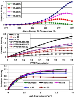
Figure 3 shows the response ofγCE estimates to variations in LAI, solar angle and transmission, and temperature. Isoprene emission increases exponentially with tem-5

perature up to a maximum that is dependent on the average temperature that the canopy has experienced during the past 240 h. Both the magnitude of the emissions and the temperature at which the maximum occurs are dependent on the past tem-perature. The result is that MEGAN predicts lower (higher) isoprene emissions in cool (warm) climates than would be simulated by the Guenther et al. (1993) algorithms. 10

However, MEGAN predictions of the isoprene emission response to short term (<24 h) temperature variations is often less than that predicted by models that do not calculate leaf temperature, e.g., BEIS2/BEIS3 or Guenther et al. (1995). This is because leaf transpiration tends to result in leaf temperature increases that are less than ambient temperature increases.

15

Above canopy PPFD is determined by solar angle and transmission. MEGAN esti-mates ofγCE increase nearly linearly with PPFD transmission for canopies that have experienced high PPFD levels (e.g., 24 h average of 600µmol m−2s−1for sun leaves) during the past day. The emission increase begins to saturate at high PPFD trans-mission for low solar angles or if the average PPFD has been low during the previous 20

day.

Figure 3 shows that estimated isoprene emission increases nearly linearly with LAI until LAI exceeds∼1.5 and is nearly constant for LAI>5. The relationship between LAI andγCE depends on solar angle and on canopy characteristics, which differ with PFT type. Isoprene emissions from canopies with clumped leaves increase relatively slowly 25

(19)

ACPD

6, 107–173, 2006

emissions

A. Guenther et al.

Title Page

Tables Figures

◭ ◮

Back Close

Full Screen / Esc

Print Version

EGU

3.2.2. Leaf age

Leaves begin to photosynthesize soon after budbreak but isoprene is not emitted in substantial quantities for days after the onset of photosynthesis (Guenther et al., 1991). In addition, old leaves eventually lose their ability to photosynthesize and produce iso-prene. Guenther et al. (1999a) developed a simple algorithm to simulate the reduced 5

emissions expected for young and old leaves based on the observed change in foliar mass over a month. An increase in foliage was assumed to imply a higher proportion of young leaves while decreasing foliage was associated with the presence of older leaves. This algorithm required a time step of one month, assumed that young leaves and old leaves had the same emission rate, and included variables that could not eas-10

ily be quantified. The following procedures to account for leaf age effects on isoprene emission estimates reduce these deficiencies.

MEGAN divides the canopy into four fractions: new foliage that emits negligible amounts of isoprene (Fnew), growing foliage that emits isoprene at less than peak rates (Fgro), mature foliage that emits isoprene at peak rates (Fmat) and senescing foliage 15

that emits isoprene at reduced rates (Fsen). The canopy-weighted average factor is calculated as

γage=FnewAnew+FgroAgro+FmatAmat+FsenAsen (10)

whereAnew (=0.05), Agro (=0.5), Amat (=1.1), and Asen (=0.4) are the relative emis-sion rates assigned to each canopy fraction. The values of these emisemis-sion factors are 20

based on the observations of Petron et al. (2001), Goldstein et al. (1998), Monson et al. (1994), Guenther et al. (1991) and Karl et al. (2003).

The canopy is divided into leaf age fractions based on the change in LAI between the current time step (LAI_c) and the previous time step (LAI_p). In cases where LAI_c=LAI_p thenFmat=1 and all other fractions (F_new,F_gro,F_sen) are equal to zero. When LAI_p>LAI_c 25

then Fnew and Fgro are equal to zero, Fsen is estimated as [(LAIp–LAIc)/LAIp] and

(20)

ACPD

6, 107–173, 2006

emissions

A. Guenther et al.

Title Page

Tables Figures

◭ ◮

Back Close

Full Screen / Esc

Print Version

EGU

calculated as

Fnew=1−(LAIp/LAIc) for t <=ti (11a)

Fnew=[ti/t][1−(LAIp/LAIc)] for t > ti (11b)

Fgro =0 for t <=ti (11c)

Fgro =[(tg−ti)/t][1−(LAIp/LAIc)] for t > ti (11d)

5

Fmat=(LAIp/LAIc) for t <=tm (11e)

Fmat=(LAIp/LAIc)+[(t−tm)/t][1−(LAIp/LAIc)] for t > tm (11f)

wheret is the length of the time step (days) between LAI_c and LAI_p,t_i is the number of days between budbreak and the induction of isoprene emission,tm is the number of

days between budbreak and the initiation of peak isoprene emission rates, andtg=tm

10

fort>t_m and t_g=t fort<=t_m. The time step, t, depends on the LAI database that is

used but generally is between 7 and 31 days. Petron et al. (2001) grew plants under conditions typical of temperate regions and observed an emission pattern that suggests at_i of about 12 days andt_mof about 28 days. Goldstein et al. (1998) field observations in a temperate forest indicate a similar value fort_m. Monson et al. (1994) found thatt_i

15

andtm are temperature dependent and are considerably less for vegetation growing at

high temperatures. These observations suggest that the temperature dependence of these variables can be estimated as

ti =5+(0.7·(300−Tt)) (12)

t_m=2.3·ti (13)

20

(21)

ACPD

6, 107–173, 2006

emissions

A. Guenther et al.

Title Page

Tables Figures

◭ ◮

Back Close

Full Screen / Esc

Print Version

EGU

are∼5% lower than estimates based on a variable ti. However, the emission rates

estimated using variableti and tm can be as much as 20% higher in tropical regions

and 20% lower in boreal regions when foliage is rapidly expanding. The differences are more pronounced when LAI variations have a higher time resolution (i.e., weekly rather than monthly).

5

3.2.3. Soil moisture

Plants require both carbon dioxide and water for growth. Carbon dioxide is taken up through leaf stomatal openings and water is obtained from the soil. However, large quantities of water are lost through stomata creating a need for adequate soil mois-ture in order to continue carbon uptake. Field measurements have shown that plants 10

with inadequate soil moisture can have significantly decreased stomatal conductance and photosynthesis, in comparison to well-watered plants, and yet can maintain ap-proximately the same isoprene emission rates (Guenther et al., 1999b). However, isoprene emission does begin to decrease when soil moisture drops below a certain level and eventually becomes negligible when plants are exposed to extended severe 15

drought (Pegoraro et al., 2004). MEGAN simulates the response of isoprene emission to drought through two mechanisms. Isoprene emissions are indirectly influenced by the soil moisture dependence of stomatal conductance which influences the leaf tem-perature estimated by the MEGAN canopy environment model. In addition, MEGAN includes an emission activity factor, dependent on soil moisture, estimated as

20

γ_SM=1 for θ > θ₁ (14a)

γSM=(θ−θw)/∆θ1 for θw < θ < θ1 (14b)

γSM=0 for θ < θw (14c)

(22)

ACPD

6, 107–173, 2006

emissions

A. Guenther et al.

Title Page

Tables Figures

◭ ◮

Back Close

Full Screen / Esc

Print Version

EGU

(=0.06) is an empirical parameter based on the observations of Pegoraro et al. (2004), andθ1=θw+∆θ1. MEGAN uses the high resolution (∼1 km

2

) database developed by Chen and Dudhia (2001) which assigns θ_w values that range from 0.01 for sand to 0.138 for clay soils. Soil moisture varies significantly with depth and the ability of a plant to extract water is dependent on root depth. We follow the PFT dependent approach 5

described by Zeng (2001) to determine the fraction of roots within each soil layer and use the weighted averageγSMfor each soil layer.

3.2.4. Other factors that influence isoprene emission activity

Isoprene emission activity can also be influenced by other environmental conditions including ozone (Velikova et al., 2005) and carbon dioxide (Buckley, 2001; Rosenstiel et 10

al., 2003) concentrations, nitrogen availability (Harley et al., 1994), and physical stress (e.g., Alessio et al., 2004). In addition, there may be significant diurnal variations that are not entirely explained by variations in environmental conditions (Funk et al., 2003). Emission activity factors accounting for these processes will be included in MEGAN as more reliable algorithms are developed. Existing observations have been used to 15

qualitatively assess the importance of these factors and are discussed in Sect. 7.

3.3. Canopy loss and production,ρ

Chemicals emitted into the canopy airspace do not always escape to the above-canopy atmosphere. Some molecules are consumed by biological, chemical and physical pro-cesses on soil and vegetation surfaces while others react within the canopy atmo-20

sphere. Some emissions escape to the above-canopy atmosphere in a different chem-ical and/or physchem-ical (i.e. gas to particle conversion) form. Theε defined by MEGAN is a net canopy emission factor but is not the net flux. This is because the MEGAN isopreneεaccounts for isoprene losses on the way out of the canopy but does not ac-count for isoprene deposition from the above-canopy atmosphere. The net ecosystem-25

(23)

ACPD

6, 107–173, 2006

emissions

A. Guenther et al.

Title Page

Tables Figures

◭ ◮

Back Close

Full Screen / Esc

Print Version

EGU

estimate and an isoprene deposition rate based on the above canopy concentration and a deposition velocity.

Inverse modeling of within-canopy gradients of isoprene suggests that at least 90% of the isoprene emitted by tropical and temperate forests escapes to the above-canopy atmosphere (Karl et al., 2004; Stroud et al., 2005). The remainder is removed through a 5

combination of chemical losses and dry deposition. While ambient mixing ratios within the canopy and roughness layer can change on the order of 10–30% due to chemistry (Makar et al., 1999), the bias of canopy scale isoprene flux measurements is small (i.e., on the order of 5–10%). This can be attributed to (1) near field effects within the canopy and (2) limited processing time between the location of isoprene emission (occurring 10

mostly within the upper canopy) and the top of the canopy. Comparisons between canopy-scale emissions based on leaf-level emission measurements extrapolated with a canopy environment model and above-canopy flux measurements tend to show that any loss of isoprene is less than the uncertainty associated with these two approaches (Guenther et al., 2000).

15

MEGAN includes a canopy loss and production factor, ρ, that is equal to unity for standard conditions and varies with changes in canopy residence time and iso-prene lifetime which is determined by canopy oxidative capacity. Variations in isoiso-prene canopy production and loss are estimated as

ρ=ρo−H/[λ·u∗·τ+H] (15)

20

where H is canopy height (m), u* is friction velocity (m s−1_), _τ _{is the above canopy}

isoprene lifetime (s),λ(=1.5±0.1) andρo(=1.01) are empirically determined

parame-ters. Equation (15) was parameterized with the above-canopy isoprene lifetime, rather than the within-canopy lifetime, because this is the value more readily available for re-gional and global modeling. Standard conditions (ρ=1) are defined as u*=0.5 m s−1, 25

τ=3600 s and H=30 m. Since variations in ρ for isoprene are typically less than 5%,

(24)

ACPD

6, 107–173, 2006

emissions

A. Guenther et al.

Title Page

Tables Figures

◭ ◮

Back Close

Full Screen / Esc

Print Version

EGU

profiles obtained during recent tropical and temperate forest field studies (Karl et al., 2004, Stroud et al., 2005). The variation of the isoprene lifetime inside the canopy was scaled to the above-canopy lifetime and based on measured O3profiles and modeled OH and NO3levels reported by Stroud et al. (2005). A random walk model similar to the one described by Baldocchi (1997) and Strong et al. (2004) was used to estimate the 5

first order decay of isoprene. Trajectories for 5000 particles were released at 4 levels (25%, 50%, 75% and 100% of canopy height) and computed for typical daytime condi-tions. The chemical loss by the ensemble mean was used to assessρintegrated over the whole canopy. A sensitivity analysis indicated that canopy height, friction velocity and lifetime were the most important variables controllingρ. Model simulations were 10

performed for a range of canopy heights (13.5 m, 27 m and 54 m), isoprene lifetimes (1370 to 6870 s) and friction velocities (0.1 to 2 m s−1).

Model simulations of the impact of isoprene on atmospheric chemistry depend on es-timates of net isoprene emission as well as eses-timates of the regional uptake of isoprene and its oxidation products, e.g. methylvinylketone, methacrolein and peroxyacetyl ni-15

trate (PAN), from the above-canopy atmosphere. Karl et al. (2004) conclude that cur-rent model procedures can underestimate the uptake of these oxidation products which would cause an overestimate of the impact of isoprene on oxidants and other atmo-spheric constituents. They also report that isoprene oxidation products deposit more rapidly during night than predicted by standard dry deposition schemes. During day-20

time, the net effect of deposition and in-canopy production of these compounds can be on the same order. These observations raise the possibility that various products of isoprene chemistry are taken up by the forest canopy more efficiently then previously assumed. This could lead to an incorrect characterization of the impact of isoprene by chemistry and transport models that have correctly simulated isoprene emission rates 25

(25)

ACPD

6, 107–173, 2006

emissions

A. Guenther et al.

Title Page

Tables Figures

◭ ◮

Back Close

Full Screen / Esc

Print Version

EGU

4. Driving variables

The MEGAN algorithms described in Sect. 3 require estimates of landcover (LAI and PFT distributions) and weather (solar transmission, air temperature, humidity, wind speed, and soil moisture). The driving variables used for MEGAN are described in this section and are compared with alternative databases.

5

4.1. Leaf area

MEGAN requires leaf area estimates with a time step of∼4 to 40 days in order to simu-late seasonal variations in leaf biomass and age distribution. MEGAN does not assume that LAI is uniformly spread over a grid cell but assumes that foliage covers only that part of the grid cell containing vegetation. The average LAI for vegetated areas is es-10

timated by dividing the grid average LAI by the fraction of the grid that is covered by vegetation. We refer to this as LAIv (the LAI of vegetation covered surfaces) and we set an upper limit of LAIv=8 to eliminate the very high values that can be estimated for grids with very little vegetation. The standard MEGAN LAIv database (MEGAN-L) was estimated by this approach using the LAI estimates of Zhang et al. (2004) and 15

estimates of vegetation cover fraction from Hansen et al. (2003).

Figure 4 illustrates how LAIv variations with time and location result in isoprene emis-sion variations of more than an order of magnitude, independent of variation in other driving variables which are held constant in these simulations. These emission vari-ations are driven by changes in only leaf age and quantity. Isoprene is reduced by 20

more than 80% at higher latitudes in winter but varies only∼15% for croplands, forests and grasslands during the growing season. Most of the extra-tropical regions of the southern hemisphere do not exceed a level of∼30% of the maximum emission while tropical forests regions rarely fall below a level of 70%.

Table 2 includes descriptions of six LAI databases that have been used to estimate 25

(26)

ACPD

6, 107–173, 2006

emissions

A. Guenther et al.

Title Page

Tables Figures

◭ ◮

Back Close

Full Screen / Esc

Print Version

EGU

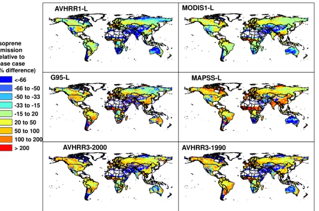
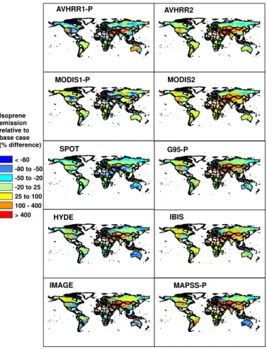
allow predictions of past and future emissions. The MEGAN-L database contains monthly estimates for years 2000 to 2004 at 30 s (∼1 km2) resolution. Table 2 in-cludes a comparison of annual global isoprene emissions estimated with alternative LAIv databases. The estimates range from 11% lower to 29% higher than the MEGAN-L values. Some of the differences are due to interannual variations, which can be seen 5

in Fig. 5 by the comparison of July average isoprene emissions estimated with the AVHRR3 databases for years 1990 and 2000. The emission estimates using MODIS based estimates of LAI, including the MEGAN-L database, are generally∼20% lower than emission estimates using the other LAI databases. All of the databases shown in Fig. 5 have regions of more than a factor of 3 lower emissions and regions with more 10

than a factor of 3 higher emissions. However, the regions with the greatest percent differences tend to be areas with relatively low emissions.

4.2. PFT distributions

The PFT databases described in Table 2 use a variety of inputs including satellite observations, vegetation inventories, ecosystem maps, and ecosystem model output. 15

The satellite data provide the highest spatial and temporal resolution while models can be used to simulate future scenarios. Vegetation inventories based on field observa-tions are expected to provide the most accurate estimates of PFT distribuobserva-tions but they have limited coverage.

Landcover data were processed to generate the MEGAN PFT categories from each 20

data source shown in Table 2. Landcover data that included PFT estimates (AVHRR1-P, MODIS1-P), were converted into the MEGAN PFT scheme with a straightforward collapsing of the fifteen PFTs into the six MEGAN PFTs. The ecosystem scheme databases (HYDE, GED, IBIS, IMAGE, MODIS2, SPOT) contain a discrete landcover type for each location that are based on either observed vegetation distribution maps, 25

(27)

ACPD

6, 107–173, 2006

emissions

A. Guenther et al.

Title Page

Tables Figures

◭ ◮

Back Close

Full Screen / Esc

Print Version

EGU

40% fineleaf evergreen trees, 1% fineleaf deciduous trees, 1% shrubs, 1% crops, 2% herbaceous and 15% bare ground or water. The PFT assignments were based on qualitative descriptions of the ecosystems and are somewhat subjective. The IMAGE database includes estimates for years 2000 and 2100 and the HYDE database has estimates for 50 year intervals between 1700 and 1950 and 20 year intervals between 5

1950 and 1990. The AVHRR2 and MODIS3 databases use satellite derived tree cover data that include total cover, deciduous and broadleaf fractions and provide the most direct estimates for the MEGAN tree PFTs and constrain the total fraction assigned to the other three MEGAN PFTs. The standard MEGAN PFT database (MEGAN-P) combines the MODIS3 database with available quantitative tree inventories based 10

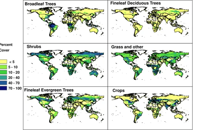
on ground observations (e.g., Kinnee et al., 1997). The global distribution of each PFT in the MEGAN database is shown in Fig. 6. The regions dominated by broadleaf trees are the major global isoprene sources. Shrubs dominate at high latitudes, where, despite relatively high emission factors, cool weather generally results in low isoprene emissions. However, shrubs have a fairly wide global distribution and so contribute to 15

isoprene emissions in many regions.

Global vegetation cover area estimated with the eleven databases range from about 90 to 120×106km2, which represents ∼60 to 80% of the global land surface (Ta-ble 1). Most of the PFT database estimates are within ∼10% of the mean value of 104×106km2. While there is considerable variation in estimates of crops, grass/other 20

and fineleaf deciduous tree areas, these PFTs make only a small contribution to the global total isoprene emission. Shrub and fineleaf evergreen tree area estimates from the different PFT databases agree relatively well. Area estimates of broadleaf trees, which contribute over half of the total global isoprene emission, are more variable and thus are a significant component of the overall uncertainty in global annual emissions. 25

(28)

ACPD

6, 107–173, 2006

emissions

A. Guenther et al.

Title Page

Tables Figures

◭ ◮

Back Close

Full Screen / Esc

Print Version

EGU

both lower and higher emission so that the global total difference (Table 2) ranges only from 13% lower to 24% higher than the value estimated with the MEGAN-P database. Ecosystem databases can be used to generate reasonable estimates of annual global isoprene emissions but may not produce accurate regional distributions. For example, the 72 ecosystem types in the GED database used for the Guenther et 5

al. (1995) emission inventory were assigned PFT distributions that resulted in a global annual emission within a few percent of the MEGAN-P database, but Fig. 7 shows that there are large regional di_fferences.

Global total emissions from all of the databases derived directly from 1 km resolu-tion data agree reasonably well. However, large global total differences in PFT area 10

estimates occur among databases that are based on MODIS observations but use different procedures to assign PFT areas. This indicates that the method for assign-ing PFT cover has a greater effect than the satellite sensor that is used. Approaches (e.g. DeFries et al., 2000) that use continuous vegetation fields (e.g. percent tree cover, percent broadleaf vegetation, percent herbaceous cover) could result in more accurate 15

PFT distributions.

4.3. Weather

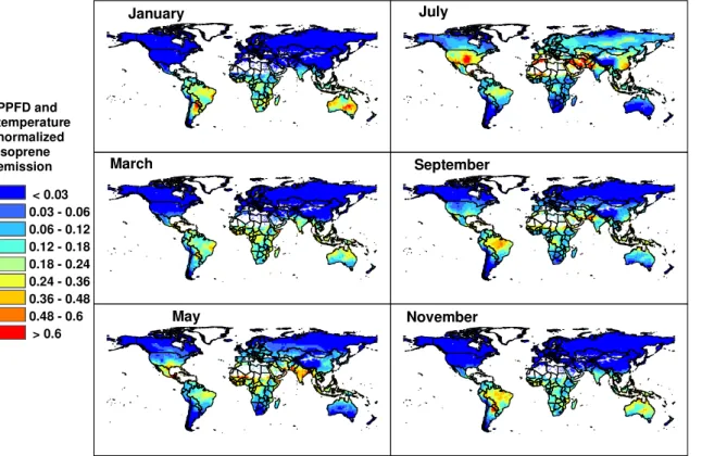
MEGAN weather input variables include ambient temperature, PPFD transmission, hu-midity, wind speed and soil moisture. Figure 8 shows that both seasonal and spatial weather variations can result in monthly average isoprene emission estimates that vary 20

by more than an order of magnitude. In particular, the cool weather conditions at high latitudes result in much lower isoprene emissions. Previous estimates of seasonal variations in tropical rainforests indicate fairly constant monthly emission rates (Guen-ther et al., 1995) but MEGAN estimates much larger (factor of 3) variations. These large seasonal variations are a result of the MEGAN algorithms that account for the 25

(29)

ACPD

6, 107–173, 2006

emissions

A. Guenther et al.

Title Page

Tables Figures

◭ ◮

Back Close

Full Screen / Esc

Print Version

EGU

needed for a rigorous evaluation.

The sensitivity of MEGAN hourly isoprene emission estimates to di_fferent global weather data was examined using the databases listed in Table 2. These include estimates based on interpolated observations (IIASA and CRU), estimates from global weather models with assimilated observations (NCEP-DOE reanalysis and MM5), and 5

two global climate models (HadCM2 and CSM1). The NCEP-DOE reanalysis, which is the only one that included soil moisture, was used as the standard database (MEGAN-W). The NCEP-DOE soil moisture was used to estimateγSMfor all emission estimates. Hourly estimates were generated from 4 times daily values for MEGAN-W, MM5 and CSM1 data and from monthly mean values for IIASA, CRU and HadCM2. Hourly tem-10

perature and PPFD variations were estimated for an average day for each month for the latter databases. Annual global emission estimates for the five alternative databases are all within −11% to +15% of the MEGAN-W estimate. The alternative weather databases result in annual global emission estimates are within∼15% of the MEGAN-W estimate. However, regional estimates differ by as much as a factor of two to three 15

for specific locations and months. The difference in isoprene emission estimated for alternatives of the same database type (e.g., observations) is similar to the level of difference between database types (e.g., observations compared to climate models).

The Guenther et al. (1995) isoprene emission estimates used the IIASA database without including diurnal temperature variations (which underestimated emissions) but 20

also used a method for estimating PPFD from cloud cover (based on Pierce and Wal-druff, 1991) that overestimated emissions. The two compensating errors resulted in an annual global emission estimate that is within∼3% of the annual global emission that is estimated when using a diurnal temperature range and more accurate estimates of surface solar radiation.

25

(30)

ACPD

6, 107–173, 2006

emissions

A. Guenther et al.

Title Page

Tables Figures

◭ ◮

Back Close

Full Screen / Esc

Print Version

EGU

occurred in regions that have moderate to high total annual precipitation but also have dry seasons with little rainfall.

5. MEGAN-EZ model description

Application of the MEGAN algorithms (Sect. 3) and the associated driving variables (Sect. 4) may require more e_ffort than is desirable for some modeling studies. We 5

have developed a simplified approach, referred to as MEGAN-EZ, with relatively sim-ple methods for estimating the three factors used to estimate emissions with Eq. (1). The factor,ρ, is simply assigned a constant value of unity. Instead of calculating land-scape average ε from the PFT specific emission factors described in Sect. 3.1 and the MEGAN-P PFT distribution database described in Sect. 4.2, a global gridded av-10

erageεcan be downloaded from the MEGAN data portal. The global distribution of

εis shown in Fig. 9 with a base resolution of 30 s (∼1 km). Global hotspots include the southeastern U.S. and southeastern Australia. Figure 9 illustrates the considerable variation inεthat occurs on both global and regional (10–100 km) scales. The small scale variability estimated by MEGAN is important for regional modeling simulations 15

due to the short lifetime of isoprene and the non-linear chemistry that determines the impact of isoprene on the chemistry of the atmosphere.

The MEGAN-EZ approach for estimating the isoprene emission activity factor is as follows,

γ=γ_LAI·γP·γT (16)

20

(31)

ACPD

6, 107–173, 2006

emissions

A. Guenther et al.

Title Page

Tables Figures

◭ ◮

Back Close

Full Screen / Esc

Print Version

EGU

tions is simulated as

γ_P =Sin(a)[1+0.0005·(P P F Dm−400)][2.46φ−(0.9φ2)] (17)

wherePPFDm is monthly average PPFD (µmol m−2_s−1_), _a _{is solar angle (degrees)}

and φ is PPFD transmission (non-dimensional) which can be estimated from solar angle and PPFD or cloud cover. The MEGAN-EZ temperature response factor,γT, is 5

estimated as

γT=Eopt·exp(0.08(Tmon−297))[CT2·exp(CT1·x)/(CT2−CT1·(1−exp(CT2·x)))] (18)

where x=[(1/Topt)–(1/Thr)]/0.00831, Thr is hourly average air temperature (K), Tmon is monthly average air temperature (K),Eopt(=1.75),CT1(=80),CT2(=200), are empirical coefficients and Toptis estimated using Eq. (8). Emission responses to LAI variations 10

are estimated as

γLAI=0.49LAI/[(1+0.2LAI2)0.5]. (19)

When the standard MEGAN driving variables are used, the annual global isoprene emission estimated by MEGAN-EZ is within∼5% of the value estimated by MEGAN. However, differences can exceed 25% for estimates at specific times and locations. 15

6. Isoprene emission estimates

Guenther et al. (1995) estimated a global annual emission of ∼570 Tg of isoprene (503 Tg of carbon), which was somewhat higher than prior estimates which had ranged from∼200–500 Tg of isoprene. The higher emission estimate of Guenther et al. (1995) is primarily due to increased emission factors, although there were also substantial dif-20