Exploring errors in paleoclimate proxy reconstructions using Monte Carlo simulations: paleotemperature from mollusk and coral geochemistry

(1)

CPD

7, 2477–2510, 2011

Exploring errors in paleoclimate proxy reconstructions

M. Carr ´e et al.

Title Page

Abstract Introduction

Conclusions References

Tables Figures

◭ ◮

Back Close

Full Screen / Esc

Printer-friendly Version Interactive Discussion

Discussion

P

a

per

|

Dis

cussion

P

a

per

|

Discussion

P

a

per

|

Discussio

n

P

a

per

Clim. Past Discuss., 7, 2477–2510, 2011 www.clim-past-discuss.net/7/2477/2011/ doi:10.5194/cpd-7-2477-2011

Climate of the Past Discussions

This discussion paper is/has been under review for the journal Climate of the Past (CP). Please refer to the corresponding final paper in CP if available.

Exploring errors in paleoclimate proxy

reconstructions using Monte Carlo

simulations: paleotemperature from

mollusk and coral geochemistry

M. Carr ´e1, J. P. Sachs2, J. M. Wallace3, and C. Favier1

1

Institut des Sciences de l’Evolution, CNRS-UM2-IRD, UMR5554, Universit ´e Montpellier 2, Pl. Eug `ene Bataillon, 34095 Montpellier, France

2

University of Washington, School of Oceanography, Box 355351, Seattle, WA 98195, USA 3

University of Washington, Department of Atmospheric Sciences, Box 351640, Seattle, WA 98195, USA

Received: 3 July 2011 – Accepted: 14 July 2011 – Published: 1 August 2011

Correspondence to: M. Carr ´e (matthieu.carre@univ-montp2.fr)

(2)

CPD

7, 2477–2510, 2011

M. Carr ´e et al.

Title Page

Tables Figures

◭ ◮

Back Close

Full Screen / Esc

Discussion

P

a

per

|

Dis

cussion

P

a

per

|

Discussion

P

a

per

|

Discussio

n

P

a

per

|

Abstract

Reconstructions of the past climate from proxy records involve a wide range of un-certainties at every step of the process. These unun-certainties and the subsequent error bar in the reconstruction of a paleoclimatic variable need to be understood and quantified in order to properly interpret the reconstructed variability and to

per-5

form meaningful comparisons with climate model outputs. Classic proxy calibration-validation techniques are not well-suited for identifying the causes of reconstruction errors, estimating their relative contribution, or understanding how errors accumulate from a multitude of sources. In this study, we focus on high resolution proxy records based on calcium carbonate geochemistry of sessile organisms such as mollusks,

10

corals, or sclerosponges, and propose an approach based on Monte Carlo simula-tions with simple numerical surrogate proxies. A freely available algorithm (MoCo, http://www.isem.cnrs.fr/spip.php?rubrique472) is provided for estimating systematic and standard errors of mean temperature, seasonality and variance reconstructed from marine accretionary archive geochemistry. This algorithm is then used for sensitivity

15

experiments in a case study to characterize and quantitatively evaluate the sensitiv-ity of systematic and standard errors to sampling randomness, stochastic uncertainty sources and systematic proxy limitations. The results of the experiments yield an il-lustrative example of the range of variations that climate reconstruction errors may undergo, and bring to light their complexity. One of the main improvements of this

20

method is the identification and estimation of systematic bias that would not otherwise be detected. It thus offers the possibility of correcting the proxy-based climate from these biases for a more accurate reconstruction. Beyond the findings of error sources for coral and mollusk-based reconstructions, our study demonstrates that numerical simulations based on Monte Carlo analyses are a simple and powerful approach to

25

(3)

CPD

7, 2477–2510, 2011

M. Carr ´e et al.

Title Page

Tables Figures

◭ ◮

Back Close

Full Screen / Esc

Discussion

P

a

per

|

Dis

cussion

P

a

per

|

Discussion

P

a

per

|

Discussio

n

P

a

per

much more comprehensive and therefore closer to reality than error estimates provided by typical calibration studies.

1 Introduction

Reconstructions of the past climate from proxy records involve a wide range of uncer-tainties at every step of the process. These unceruncer-tainties and the subsequent error bar

5

in the reconstruction of a paleoclimatic variable need to be understood and quantified in order to properly interpret the reconstructed variability and to perform meaningful comparisons with climate model outputs. In a recent overview of methods used in high resolution paleoclimatology, Hughes and Ammann (2009) concluded that “the study of the processes by which climate proxy records are formed [. . . ] should be accorded high

10

priority”. Highly complex methods based on Bayesian statistics and involving biological models have been developed for pollen assemblages that provide a probability distri-bution of the paleoclimate reconstruction (Guiot et al., 2009). Considerable effort has also been devoted to statistically estimate the sensitivity of climate field reconstructions from tree rings to proxy uncertainties, the proxy network, and the calculation methods

15

(Mann et al., 2005, 2007; Lee et al., 2008; Riedwyl et al., 2009). For many other proxies, and especially in paleo-oceanography, the climate proxy development work has been concentrated on the calculation of empirical regression models (or transfer functions) linking the proxies to the environmental variables. Then, in most studies, the uncertainty of the paleo-oceanographic variable reconstruction is estimated by the

20

scattering of the empirical calibration dataset. Thus, in these cases, the reconstruction error bar is assumed to be identical in every application of the transfer function. We ar-gue that, although essential, the empirical calibration-verification work only provides a first-order, generally underestimated, value of the error bar. The processes leading to a climate proxy record involve randomness and a suite of stochastic parameters

operat-25

(4)

CPD

7, 2477–2510, 2011

M. Carr ´e et al.

Title Page

Tables Figures

◭ ◮

Back Close

Full Screen / Esc

Discussion

P

a

per

|

Dis

cussion

P

a

per

|

Discussion

P

a

per

|

Discussio

n

P

a

per

|

number of tests in a calibration-verification approach. There is growing agreement in the paleoclimate science community on the need for better methods to evaluate the uncertainties in climate proxy records (Jones et al., 2009).

In this study, we focus on high resolution proxy records based on calcium carbon-ate geochemistry of sessile organisms such as mollusks, corals, or sclerosponges.

5

Short-term windows of monthly to decadal sea surface temperature (SST) can be re-constructed from these accretionary archives using paleo-temperature proxies such as Sr/Ca (Beck et al., 1992; Marshall and McCulloch, 2002; Corr ège et al., 2004; Rosen-heim et al, 2004) orδ18O (Epstein et al., 1953; Grossman and Ku, 1986, B öhm et al., 2000; Carr é et al., 2005) serially measured along the growth axis. In most works based

10

on this technique, SSTs are calculated using an empirical regression model, verified with modern samples. The same error bar, assumed to be inherent to the proxy re-gression model, is ascribed to all data points. However, paleoclimatic interpretations are not based on a single data point, but rather on characteristics of the whole dataset (mean, variance, spectral power density), which is taken to be representative of the

15

mean climate of a time period over a defined region. Even considering that the error bar was correctly estimated for single SST reconstructions, it is not readily applied to the statistical properties of the dataset. Here we develop a quantitative framework for evaluating how stochastic noise (analytic error, vital effect, weather, microenvironment heterogeneity, growth breaks . . . ) and proxy-specific noise (physiological temperature

20

tolerance, spawning growth breaks . . . ) influence the statistical properties of paleocli-mate data derived from mollusk, coral, and coralline sponge geochemistry.

We propose an approach based on Monte Carlo simulations with simple numeri-cal surrogate proxies. Monte Carlo simulations have been used in previous studies (Briskin and Harrell, 1980; Ballentine and Hall, 1999; Touchan et al., 1999; Meibom et

25

(5)

CPD

7, 2477–2510, 2011

M. Carr ´e et al.

Title Page

Tables Figures

◭ ◮

Back Close

Full Screen / Esc

Discussion

P

a

per

|

Dis

cussion

P

a

per

|

Discussion

P

a

per

|

Discussio

n

P

a

per

of stochastic parameters, and how it can significantly improve the understanding of the proxy signal and eventually the quality of the paleoclimate reconstruction. This tech-nique is conceptually very simple compared to the full probabilistic modelling studies using Bayesian inferences that have been developed by statisticians for climate field reconstructions (Haslett et al., 2006; Jones et al., 2009). It is intended for use as an

5

intermediate method, efficient enough to provide reliable assessments of paleoclimate errors, while being technically and conceptually accessible to a broad community in paleoclimate science.

Specifically, we provide a ready-to-use, parameterize-yourself, open access algo-rithm for estimating systematic and standard errors of mean temperature, seasonality

10

and variance reconstructed from marine accretionary archive geochemistry (mollusks, corals, sclerosponges . . . ). This algorithm is then used in a case study to characterize and quantitatively evaluate the sensitivity of systematic and standard errors to sampling randomness, stochastic uncertainty sources and systematic proxy limitations.

2 The surrogate paleoclimate proxy Monte Carlo algorithm for mollusks and

15

corals (MoCo)

The starting hypothesis is that an empirical linear regression model, with no apparent systematic bias, is available for the calculation of a climate variable from a single geo-chemical proxy. This would thus apply to quaternary temperature reconstructions from Sr/Ca ratios measured in corals (Beck et al., 1992) and sclerosponges (Rosenheim et

20

al., 2004), or to temperature reconstructions from coral δ18O (Cobb et al., 2003) or mollusk shellδ18O (Sch ¨one et al., 2004) in conditions where the water isotopic compo-sition can be constrained. As in all surrogate proxy (also referred to as “pseudo-proxy”) studies, the basic principle is to use a realistic climate time series, sample and perturb it in a way that mimics the proxy uncertainties, and compare the surrogate

“recon-25

(6)

CPD

7, 2477–2510, 2011

M. Carr ´e et al.

Title Page

Tables Figures

◭ ◮

Back Close

Full Screen / Esc

Discussion

P

a

per

|

Dis

cussion

P

a

per

|

Discussion

P

a

per

|

Discussio

n

P

a

per

|

2.1 Different types of error

We explore both systematic and standard errors of statistical climate properties [annual meanT_m, variance of the annual mean var(T_m), mean annual amplitude∆T, variance of the annual amplitude var(_∆T)] reconstructed from a random sample of specimens taken to be representative of a time period.T refers here to the reconstructed

environ-5

mental variable, which could be temperature, salinity, pH or something else. Identifying and estimating systematic errors allows us to correct the reconstruction and improve its accuracy. A quantitative estimate of the standard deviation is also essential to de-termine a threshold of significance in the amplitude of the climate proxy variations.

Defining the error in a paleoclimate reconstruction from a local archive is not trivial.

10

It may depend on the climate information sought. An ideal proxy would provide the exact temperature in a precise location and thus be considered as error-free, but if the aim is to have regional scale information, the proxy signal would still be noisy owing to micro-environment effects. Weather also contributes to the noise inherent in climate statistics. Thus some of the noise in the reconstruction is related to random sampling

15

in time and space and is thus independent of the quality of the empirical regression model.

The formation of the proxy record involves a complex chain of physical and biological processes (for instance mechanisms of Strontium incorporation into coral aragonite) that introduce non-climate-related stochasticity and limitations in the climate-proxy

re-20

lationship (Meibom et al., 2003). The scatter inherent in in situ calibration datasets partly captures this stochastic variability but does not allow the exploration of its full range nor the characterization of the error from different sources. Stochastic param-eters may contribute to the standard error in the reconstruction of climate statistical properties as well as to systematic errors as we will show.

25

(7)

CPD

7, 2477–2510, 2011

M. Carr ´e et al.

Title Page

Tables Figures

◭ ◮

Back Close

Full Screen / Esc

Discussion

P

a

per

|

Dis

cussion

P

a

per

|

Discussion

P

a

per

|

Discussio

n

P

a

per

carbonateδ18O is used as a paleotemperature proxy. They also include uncertainties in the proxy calibration model. Considering that the mechanisms behind such errors are identical for all specimens in the archive (which is generally assumed), then the model would be identically wrong for all the climate calculations. Therefore, the pale-oclimate errors due to the imperfection of the model do not contribute to the standard

5

error, but instead are more comparable to a systematic error (although its value might be linearly dependent on the proxy variable). Nevertheless, when the source of a po-tential systematic error can be identified, it may be possible to estimate statistically its impact on the reconstructed climate.

Owing to their different nature, and for a more complete representation of error, the

10

standard error and the potential systematic error should be represented separately in paleoclimate results (Carr ´e et al., 2011). Systematic errors that can be estimated should be corrected for. The MoCo algorithm yields estimates of the standard error, systematic error, and potential systematic error.

2.2 The Monte Carlo simulation

15

Monte Carlo techniques are useful for the analysis of complex stochastic systems (Metropolis and Ullam, 1949; Hastings, 1970). In our study, surrogate proxy records are produced by perturbing a known climate time series with a suite of random noise. Each surrogate proxy record is only of realization of the infinite number of values and combinations that noise can take. In the Monte Carlo simulation, this process is

re-20

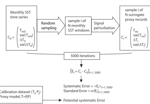
peated many times (5000 iterations in the experiments presented here) in order to have a representative sample of the range of responses, and therefore of the probability dis-tribution of the error (Fig. 1). The average value of the error population calculated in a Monte Carlo simulation represents the systematic error. If the reconstruction method is not biased, the mean value of the error population should be zero. If this is not

25

(8)

CPD

7, 2477–2510, 2011

M. Carr ´e et al.

Title Page

Tables Figures

◭ ◮

Back Close

Full Screen / Esc

Discussion

P

a

per

|

Dis

cussion

P

a

per

|

Discussion

P

a

per

|

Discussio

n

P

a

per

|

2.3 Using the MoCo.m application

MoCo.m is freely available and can be downloaded at http://www.isem.cnrs.fr/spip. php?rubrique472, along with the MoCo readme.txt file which contains step by step instructions for users. The program is designed to work with the Matlab software. The algorithm is parameterized by the user according to the specifics of the study. These

5

input parameters are listed in table 1 and described in the next section.

3 Inputs to the algorithm

3.1 A target time series

When using the MoCo algorithm, a climate time series is first chosen that will be used as the “target climate”. As will be shown later, the characteristics of the target time

10

series have a large influence on the reconstruction error. It is therefore important to use a realistic time series with a variability that is as far as possible similar to the paleoclimate that the proxy is being used to study. The length of the time series should be much longer than the typical proxy record length to allow adequate random sampling in time. For instance, if 50-yr long coral records are being used to study early Holocene

15

climate, a time series of at least 1000 yr should be used as a target in the Monte Carlo simulation. Such a long time series can only be provided by climate models. Instrumental time series may be used for short-lived proxy archives such as one-year long mollusk shells. The target time series for proxies with sub-annual resolution should be monthly, starting in January, and include full years without missing data.

20

3.2 Random sampling of target time series

(9)

CPD

7, 2477–2510, 2011

M. Carr ´e et al.

Title Page

Tables Figures

◭ ◮

Back Close

Full Screen / Esc

Discussion

P

a

per

|

Dis

cussion

P

a

per

|

Discussion

P

a

per

|

Discussio

n

P

a

per

proxy records. Two approximations are made in this process: (1) the proxy record time resolution is assumed to be monthly and constant, (2) all specimens are assumed to have the same duration equal toNy years.

3.3 Signal perturbation

In this step, the random sample ofN climate time windows is perturbed by stochastic

5

noise and by archive-related limitations.

3.3.1 Spatial heterogeneity

Corals, mollusks and sclerosponges, as sessile organisms, record only a very local en-vironmental variability that may differ from the regional environmental variability. This effect is especially significant in coastal environments where large spatial heterogeneity

10

can occur. Several specimens should thus be analyzed to average out this heterogene-ity effect. In MoCo, this stochastic noise is represented by a random parameter with a normal distribution N(0,σs). A random value is drawn for every specimen and added uniformly to the climate variable over the whole time window.

3.3.2 Monthly noise

15

MoCo provides for three additional sources of month-to-month noise: (1) the proxy analytical error, (2) the weather scale variability, (3) biogenic carbonate heterogeneity at the µm scale of microsampling owing to vital effects and diagenesis. These three types of noise follow the normal distributions N(0,σa), N(0,σw), N(0,σc) respectively, where the standard deviation are expressed in the proxy unit (e.g. mmol/mol for coral

20

(10)

CPD

7, 2477–2510, 2011

M. Carr ´e et al.

Title Page

Tables Figures

◭ ◮

Back Close

Full Screen / Esc

Discussion

P

a

per

|

Dis

cussion

P

a

per

|

Discussion

P

a

per

|

Discussio

n

P

a

per

|

normally distributed because they are expected to have symmetric distributions, and each is comprised of a large number of stochastic processes.

3.3.3 Limitations of the biological archives

The archives considered in this study, corals, mollusks, sclerosponges, coralline algae, are living organisms. Their biology constrains their growth and thus the way in which

5

they record the environment. Every species is defined by a range of physico-chemical tolerances beyond which they stop precipitating new carbonate skeletal material. If it is possible that the reconstructed variable may represent a growth limitation (like temperature or salinity) the effect of these limits should be explored and quantified. Upper and lower biological limits (Tls, Tli) for the variable T are thus considered in

10

MoCo.

Some species systematically stop growing at a precise period of the year because their resources are exclusively dedicated to reproduction. This implies a systematic gap in the record that may affect the final calculated averages or variance. Parameters gb1 to gb12 define the typical monthly growth pattern of the species (Table 1).

15

Finally, growth breaks may occur randomly because of storms, predation, or sick-ness. The MoCo program allows the choice of occurrence of zero to 12 random growth breaks per year.

3.4 Proxy model calibration dataset

Here we only consider linear regression models between the reconstructed variableT

20

(11)

CPD

7, 2477–2510, 2011

M. Carr ´e et al.

Title Page

Tables Figures

◭ ◮

Back Close

Full Screen / Esc

Discussion

P

a

per

|

Dis

cussion

P

a

per

|

Discussion

P

a

per

|

Discussio

n

P

a

per

I(alpha)=±t·_σσT

P ·

s

(1−R2)

Nc−2 , I(beta)=±t·σT·

s

(1−R2)

Nc−2 (1)

WhereNcis the number of data points in the calibration dataset,σ_T andσ_P the stan-dard deviations ofT and P respectively in the calibration dataset,R is the Pearson’s correlation coefficient, andt is the value of the Student variable at the 0.05 confidence level andNc-2 degrees of freedom.

5

4 Sensitivity experiments

Five sensitivity experiments were performed using the MoCo algorithm to explore the influence of (1) the random sampling (exp. 1 and 2), (2) stochastic perturbations (exp. 1, 2, and 3), (3) the biological limitations of the archive (exp. 4 and 5), and (4) the target time series (exp. 3, 4, and 5) on the systematic and standard errors when

reconstruct-10

ing the statistical characteristics of the target time series (T_m, var(T_m), ∆T, var(∆T)). To perform these experiments we chose the illustrative case study of temperature re-constructions in the eastern Pacific from mollusk shell oxygen isotopes. We used the empirical proxy model established by Grossmann and Ku (1986) for biogenic aragonite (Eq. 2), which is often considered as the definition of isotopic equilibrium for biogenic

15

aragonite and has been widely used for paleoclimate studies from aragonitic mollusk shells:

T(◦_C)₌₁₉_.₇₃₋₄_.₃₄₍_δ18_O

arag.−δ18Ow) (2)

δ18Oarag. and δ

18

O_w are expressed in ‰ versus the V-PDB and V-SMOW standards respectively. This proxy model is used only for the case study. Any other proxy model

20

(12)

CPD

7, 2477–2510, 2011

M. Carr ´e et al.

Title Page

Tables Figures

◭ ◮

Back Close

Full Screen / Esc

Discussion

P

a

per

|

Dis

cussion

P

a

per

|

Discussion

P

a

per

|

Discussio

n

P

a

per

|

Three sea surface temperature (SST) time series were used as “target” climatol-ogy: (1) the 1925–2002 monthly in situ instrumental record from Puerto Chicama, Peru (measured by IMARPE), (2) the 1950–2009 monthly SST time series of the Ni ˜no1+2 area (both time series are available at http://jisao.washington.edu/data sets/ #time series), and (3) the 1000-yr long monthly SST time series of the Ni ˜no1+2 area

5

from the preindustrial control simulation of the IPSL CM4v2 coupled ocean atmosphere general circulation model (GCM) (for details about the simulation, see Servonnat et al., 2010). The target time series are presented in Table 2. The first 2 time series were used in all experiments except for the experiment 2 in which the GCM time series was used (Table 3). The parameterization of the sensitivity experiments are summarized in

10

Table 3.

4.1 Experiment 1: Influence of random sampling and stochastic noise

The first experiment was designed to test the effect of sampling on the standard and systematic errors and compare it to the effect of three stochastic noises that were turned offor on. Realistic values were assigned toσs(spatial heterogeneity) andσm

15

(month-to-month noise) based on field measurements on the Peruvian coast. In this experiment, shell records span one year and no biological limitations were included.

4.2 Experiment 2: Influence of the record length

Experiment 2 was designed to explore the effect of the record length on the skill of the reconstructions considering the existence of realistic stochastic perturbations of

20

the proxy signal. No biological limitations were included. The record lengthNy ranged from 1 to 200 yr as would be expected for coral-based records, and the total number of yearsN*Ny recorded by the sample was held constant at 200 yr. No instrumental record was long enough for this experiment so a 1000 yr long pre-industrial OA-GCM simulation of the Ni ˜no1₊2 SSTs was used as a monthly target time series.

(13)

CPD

7, 2477–2510, 2011

M. Carr ´e et al.

Title Page

Tables Figures

◭ ◮

Back Close

Full Screen / Esc

Discussion

P

a

per

|

Dis

cussion

P

a

per

|

Discussion

P

a

per

|

Discussio

n

P

a

per

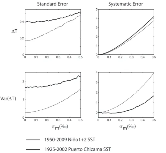
4.3 Experiment 3: Influence of month-to-month noise

Experiment 3 explored further the effect of the individual data point quality degraded by the monthly noise, characterized byσm, which includes the analytical error, weather scale noise, and skeletal carbonate heterogeneity. Here, all perturbations were turned offand all parameters were fixed except for σm which varied from 0 (ideal proxy) to

5

0.5 ‰. Simulations were performed with samples of 20 one-year long shells, and two di_fferent target time series.

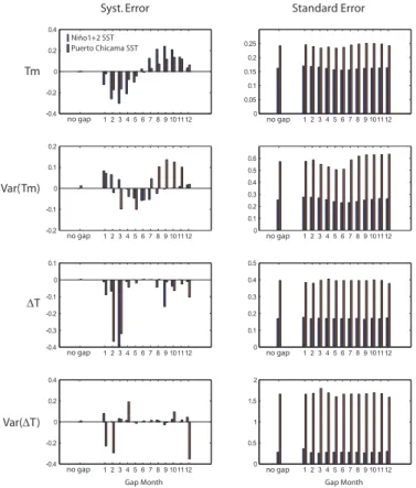
4.4 Experiment 4: Influence of a growth break

Experiment 4 was designed to test the effect of yearly growth breaks (such as spawning growth breaks) on reconstruction errors. All other perturbations were turned offand all

10

parameters exceptgbi were fixed. We only considered the case of a single one-month growth break per year, and compared the effect of varying its month of occurrence. Simulations were performed with samples of 20 one-year long shells, and with two di_fferent target time series.

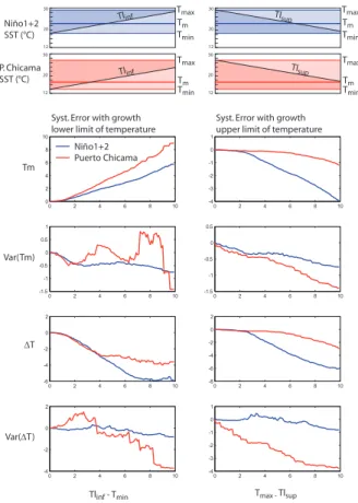
4.5 Experiment 5: influence of temperature tolerance range

15

In experiment 5, we explored the effect of temperature limits on skeletal growth for the reconstruction of two target time series. Obviously, the reconstruction would not be a_ffected if the biological temperature limits are outside the temperature range of the time series. Therefore, in this experiment, the upper (lower) temperature limit ranged from the maximum (minimum) temperatureTmax(Tmin) of the target time series toTmax

-20

10◦_{C (}_T

(14)

CPD

7, 2477–2510, 2011

M. Carr ´e et al.

Title Page

Tables Figures

◭ ◮

Back Close

Full Screen / Esc

Discussion

P

a

per

|

Dis

cussion

P

a

per

|

Discussion

P

a

per

|

Discussio

n

P

a

per

|

5 Results

5.1 Potential systematic error

The MoCo program calculates the potential systematic error due to errors in the linear proxy model calibration. This error not only depends on the proxy model but also on the target climate. When calculating the mean temperature for instance, the error

in-5

creases with the difference between the reconstructed conditions and the calibration dataset mean value. The mean valueT0 of Grossmann and Ku’s (1986) dataset was 10.5◦C. When using the Puerto Chicama time series (T_m=17.1◦C), the error for T_m reconstruction due to the proxy model only is±2.1◦C (95 % confidence level). This

error increases to±3.9◦C with the Ni ˜no1+2 time series (Tm=23.0◦C). These

uncer-10

tainties are so large because the target temperature range is far from the temperature calibration range. If the mean value of the target time series was 11◦C, the uncertainty at 95 % confidence level would only be±0.4◦C. The error for the mean seasonal

ampli-tude (∆T) was also significant for Puerto Chicama (±1.4◦C) and for Ni ˜no1+2 (±1.9◦C)

time series. This confirms the importance of local specific calibration works to minimize

15

this type of errors.

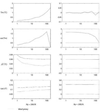
5.2 Random sampling (Exp. 1 and 2)

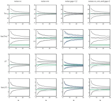
In experiment 1, the effect of random sampling is quantitatively estimated and com-pared to the stochastic proxy uncertainties (Fig. 2). The effect of sampling only is represented in Fig. 2 by the “ideal proxy” curves. It appears that random sampling is

20

one of the main sources of the standard error. This error decreases rapidly with the sample size and becomes relatively insignificant forTmand ∆T whenN reaches 20. On the other hand, the standard error for var(Tm) and var(_∆T) due to sampling remains relatively significant up toN =30.

In experiment 2, we test whether reconstructions from long proxy records are more

25

(15)

CPD

7, 2477–2510, 2011

M. Carr ´e et al.

Title Page

Tables Figures

◭ ◮

Back Close

Full Screen / Esc

Discussion

P

a

per

|

Dis

cussion

P

a

per

|

Discussion

P

a

per

|

Discussio

n

P

a

per

years recorded (N·Ny) is kept constant and equal to 200 in order to test only the

in-fluence of the record length. For regional mean temperature (Tm) reconstructions, it appears that a large sample set of short records provides a more precise estimate than a few long records. This result is due to the influence of local spatial temperature het-erogeneity which is averaged with large sample sets but represents a significant error

5

when determined from a single record. In a similar way, the spatial variance tends to overwhelm the climatic variability var(Tm) when the sample is small, unless it is calcu-lated from a single record (Fig. 3,N=1,Ny₌200). Systematic errors are only a_ffected by record length in the case of var(Tm). While the annual temperature variance is overestimated with short records because of the additional spatial variance, this effect

10

decreases when the record lengthens. Finally it appears that intermediate values ofN andNy (here 20 10-yr old shells) would yield the best compromise for accuracy and precision in the reconstruction of Tm and var(Tm). The reconstruction skills for ∆T, and var(_∆T) are not significantly a_ffected by the record length in our experiment.

5.3 Effects of stochastic noise (Exp. 1, 2, and 3)

15

Three kinds of stochastic perturbations (see Sect. 2.3.3.) are applied to the climate signal in experiments 1, 2, and 3. In the first experiment, their influence is observed separately and compared to ideal proxy reconstruction errors. As expected, spatial variability greatly affects the standard error of the Tmreconstruction (Fig. 2) and this effect increases with the record length (Fig. 3). It also induces a systematic positive

20

bias for the var(Tm) reconstruction which decreases with record length (Fig. 3). The monthly variability in experiment 1 does not significantly affect the Tmand var(Tm) re-constructions but it induces an unexpected overestimation of the annual amplitude∆T and of its variance (Fig. 2). This latter effect does not depend significantly on the record length (Fig. 3). Random growth breaks have no significant impact on the standard error

25

(16)

CPD

7, 2477–2510, 2011

M. Carr ´e et al.

Title Page

Tables Figures

◭ ◮

Back Close

Full Screen / Esc

Discussion

P

a

per

|

Dis

cussion

P

a

per

|

Discussion

P

a

per

|

Discussio

n

P

a

per

|

In our case study, the stochastic perturbation at the data point level characterized byσminvolves monthly waterδ18O variability, carbonateδ18O analytic error, and shell carbonate heterogeneity. Its effect on ∆T and var(∆T) reconstructions is further ex-plored in experiment 3 (Fig. 4) using two different target SST time series. In our ex-periment, the maximum value of σm is 0.5 ‰ (or 2.2◦_{C on the temperature scale)}

5

which represents an extremely noisy proxy record. The systematic positive bias on ∆T estimate is ∼1◦C when σm=0.1 ‰ and increases to 3◦C when σm=0.4 ‰. For

other parameters, the response depends on the target time series. Forσm=0.2 ‰, the systematic error for var(∆T) is about 100 % for the Ni ˜no1+2 time series while it is almost null for the Puerto Chicama time series. Standard errors for Ni ˜no1+2 SSTs are

10

more sensitive to the monthly noise than those for Puerto Chicama SSTs. This can be explained by the higher variability of Puerto Chicama (Table 2), which makes the noise-related variability relatively smaller.

5.4 E_ffects of biological limitations (Exp. 4 and 5)

Growth hiatuses may occur every year at approximately the same date for breeding or

15

other reasons (Sato et al., 1999). In experiment 4 (Fig. 5), we showed that the date of the growth break has little impact on the paleoclimate reconstruction standard error but may produce systematic errors. As expected, the mean annual temperature would be underestimated (overestimated) if the growth breaks occur in the warmest (coldest) period. Here, the maximum systematic error forTmwas−0.3◦C. The annual amplitude

20

may be largely underestimated if the growth hiatuses occur during seasonal extrema. In our experiment the systematic bias for∆T reached−0.4◦C with a systematic growth

break in March for the Ni ˜no1+2 SST time series. Proxy reconstructions of variances were affected by growth hiatuses in a much less predictable way. For Puerto Chicama SSTs, maximum systematic errors reached about 8 % for var(Tm) when growth breaks

25

(17)

CPD

7, 2477–2510, 2011

M. Carr ´e et al.

Title Page

Tables Figures

◭ ◮

Back Close

Full Screen / Esc

Discussion

P

a

per

|

Dis

cussion

P

a

per

|

Discussion

P

a

per

|

Discussio

n

P

a

per

Temperature tolerance for skeletal growth is an especially important biological lim-itation that may induce significant systematic biases in paleoclimate reconstructions. These biases were explored with 2 different time series in experiment 5 (Fig. 6). While it is obvious that upper (lower) temperature limits cause underestimation (overestima-tion) of the mean temperatureTm, and that _∆T is in both cases underestimated, our

5

experiment permits calculation of a quantitative estimate of this error. In experiment 5, the systematic error responses to lower and upper limits were not symmetrical. For Ni ˜no1₊2, the e_ffect of the lower temperature limit began to be significant when it reached ∼1.5◦C above the minimum temperature, whereas the effect of the upper

limit began to be significant when it reached ∼3◦C under the maximum temperature.

10

The systematic biases produced for var(Tm) and var(_∆T) reconstructions rapidly be-came significant and had unpredictable profiles, switching from positive to negative values (Fig. 6), especially for the lower temperature limit.

5.5 Importance of the target time series (exp 3, 4, and 5)

The results of experiments 3, 4, and 5 showed that the error strongly depends on

15

the climate time series used as a target in the experiment because it depends on the probability density function of the temperature. The Puerto Chicama time series has a much wider distribution than the Ni ˜no1₊2 time series (Table 2) so that standard error due to random sampling is much larger for Puerto Chicama (Fig. 4 (σm=0); Fig. 5). Target temperature distributions are also differently affected by proxy uncertainties,

20

which generates di_fferent error responses (Figs. 4, 5, 6). In the three experiments, the error responses to proxy uncertainties were strongly modulated by the character-istics of the target time series. The same proxy perturbation may induce strong errors with one time series and be insignificant with another. For instance, the upper growth temperature limit had no significant effect on the reconstruction ofTm and ∆T until it

25

reached∼6◦C under the maximum value of the Puerto Chicama SST (Fig. 6) because

(18)

CPD

7, 2477–2510, 2011

M. Carr ´e et al.

Title Page

Tables Figures

◭ ◮

Back Close

Full Screen / Esc

Discussion

P

a

per

|

Dis

cussion

P

a

per

|

Discussion

P

a

per

|

Discussio

n

P

a

per

|

location. These results show that the choice of the target time series when using MoCo to estimate paleoclimate reconstruction errors is a critical step.

6 Discussion

6.1 Implications for paleoclimate error representation

Three types of errors have been distinguished in this study that should all be treated

5

and represented explicitly. Standard error is the classic error bar. However, while the error bar is generally represented for individual data points (σmin our case study), it is generally not even mentioned for variables calculated from the whole dataset (Tm, var(Tm), ∆T, and var(∆T)), as if it was implicitly considered to be the same as for individual data points. Our experiments show how the standard error for statistical

10

characteristics (Tm, var(Tm),∆T, and var(∆T)) is related to σm(Fig. 4), but they also show how distinct and how much more complex it is. Monte Carlo simulations are reliable and simple tools to explore issues with this level of stochasticity and complexity. Systematic errors are meant to be corrected for when detected and quantified, and thus are not supposed to be represented. Systematic errors whose probability

distri-15

butions only can be estimated, referred to here as potential systematic errors, should be represented separately from the standard error. In our case study, they include the error due to flaws in the proxy model and uncertainty about the regional ice volume effect on sea waterδ18O.

6.2 Understanding the proxy

20

(19)

CPD

7, 2477–2510, 2011

M. Carr ´e et al.

Title Page

Tables Figures

◭ ◮

Back Close

Full Screen / Esc

Discussion

P

a

per

|

Dis

cussion

P

a

per

|

Discussion

P

a

per

|

Discussio

n

P

a

per

the proxy. Stochastic uncertainties and biological limitations significantly affect the re-sulting climate reconstruction, in different manners depending on the location and the climate parameter. Errors are affected by proxy uncertainties in a way that is so sensi-tive to the parameterization and to the target time series that no general relationships between errors and signal perturbations should be concluded from these experiments.

5

The results of the experiments, however, yield an illustrative example of the range of variations that climate reconstruction errors may undergo, and bring to light their com-plexity. Classic calibration-validation techniques are not well-suited for identifying the causes of reconstruction errors, estimating their relative contribution, or understanding how errors accumulate from a multitude of sources.

10

While the influences of several sources of error were qualitatively predictable, some perturbations produced significant unpredictable systematic bias (Figs. 4, 5, 6). Be-yond the findings of error sources for coral and mollusk-based reconstructions, our study demonstrates that numerical simulations based on Monte Carlo analyses are a simple and powerful approach to improve the proxy calibration process. A thourough

15

understanding of the proxy record errors is essential for the interpretation of paleocli-mate records from proxies derived from accretionary skeleton geochemistry.

6.3 Quantifying errors

Quantifying errors in paleoclimate reconstructions is essential for accurate and mean-ingful proxy-proxy and proxy-model comparisons. The MoCo algorithm was designed

20

to provide quantitative estimates of the three kinds of errors identified in Sect. 2.1 for coral and mollusk based climate reconstructions. It implies that the linear proxy model has been previously validated. The accuracy of the error quantification using MoCo may be limited in three ways:

the model for the paleoclimate reconstruction process implies simplifications

includ-25

(20)

CPD

7, 2477–2510, 2011

M. Carr ´e et al.

Title Page

Tables Figures

◭ ◮

Back Close

Full Screen / Esc

Discussion

P

a

per

|

Dis

cussion

P

a

per

|

Discussion

P

a

per

|

Discussio

n

P

a

per

|

The full parameterization of MoCo by the user requires field measurements and knowledge of the organism ecology and growth. Uncertainties inσs, σm, Tli orTls estimates may affect the quantification of errors.

By definition in paleoclimatology, the true target climate is unknown, and therefore different from the target time series used in the MoCo simulation. The errors calculated

5

by the simulation are therefore not true errors but only estimates whose accuracy de-pends on the similarity between the true past climate and the target time series. In the selection process for the simulation target time series, it is recommended to seek high temporal variability so that errors will not be underestimated. Despite these caveats, and even if the user-defined inputs are imperfect, the error estimates provided by MoCo

10

are much more comprehensive and therefore closer to reality than error estimates pro-vided by typical calibration studies. One of the main improvements of this method is the identification and estimation of systematic bias that would not otherwise be detected. It thus o_ffers the possibility of correcting the proxy-based climate from these biases for a more accurate reconstruction.

15

6.4 Extending applications

Sensitivity experiments were based on an illustrative case study of SST reconstruction from mollusk or coral δ18O in an environment where water δ18O is reasonably con-strained. The same kind of experiment would improve the understanding of other prox-ies including temperature reconstructions from Sr/Ca ratios in corals (Beck et al., 1992;

20

De Villiers et al., 1994; Marshall and McCulloch, 2002) and sclerosponges (Swart et al., 2002; Rosenheim et al., 2004), Mg/Ca ratios in coralline algae (Kamenos et al., 2008), and pH from coralδ11B (Rollion-Bard et al., 2011).

In many environments, biocarbonate δ18O variations yield a mixed signal between water temperature and waterδ18O variations related to freshwater input. Under such

25

(21)

CPD

7, 2477–2510, 2011

M. Carr ´e et al.

Title Page

Tables Figures

◭ ◮

Back Close

Full Screen / Esc

Discussion

P

a

per

|

Dis

cussion

P

a

per

|

Discussion

P

a

per

|

Discussio

n

P

a

per

water δ18O time series. This approach, referred to as forward modelling, has been applied to a variety of proxies, such as planktonic foraminiferaδ18O (Schmidt, 1999), or stalagmiteδ18O (Baker and Bradley, 2010). The strength of forward modeling that incorporates Monte Carlo analyses for paleoclimate proxy calibration was showed by Evans (2007) through a case study with wood celluloseδ18O. To our knowledge it has

5

never been applied to corals or mollusks. MoCo-type algorithms would be especially useful for exploring the error of salinity or water δ18O reconstructions based on the combination of coralδ18O and Sr/Ca ratios, since both proxies add and propagate in an unpredictable way.

7 Conclusions

10

We demonstrated that proxy climate reconstructions from biocarbonate accretionary skeleton geochemistry involve errors that are much more complex and potentially larger than those estimated from empirical calibration scatter. We showed in an illustrative case study that surrogate proxy techniques associated with Monte Carlo analyses are powerful tools to improve the understanding and calibration of proxy records.

Sensi-15

tivity experiments showed the significant and often unpredictable influence of random sampling, stochastic proxy perturbations, archive biological limitations, and the climate characteristics. These numerical experiments are a fast and e_fficient technique for a qualitative assessment of these influences and provide a first-order quantitative approx-imation of the reconstruction errors. We provided an open access Matlab algorithm,

20

MoCo.m, available at http://www.isem.cnrs.fr/spip.php?rubrique472, for quantitatively estimating the error related to the proxy linear model, systematic biases, and the stan-dard errors for proxy-based climate reconstructions. Although the algorithm is a very simple model of the climate reconstruction process, it allows significant improvement in the evaluation of the reconstruction uncertainties. Its conceptual simplicity should

al-25

(22)

CPD

7, 2477–2510, 2011

M. Carr ´e et al.

Title Page

Tables Figures

◭ ◮

Back Close

Full Screen / Esc

Discussion

P

a

per

|

Dis

cussion

P

a

per

|

Discussion

P

a

per

|

Discussio

n

P

a

per

|

Acknowledgements. This work was supported by a postdoctoral fellowship of the Joint

Insti-tute for the Study of the Atmosphere and Ocean (JISAO) under NOAA Cooperative Agreement No. NA17RJ1232, by the US National Science Foundation under grant No NSF-ATM-0811382 (J.P.S.), and by the US National Oceanic and Atmospheric Administration under grant #

pro-5

gramming. We also thank three anonymous reviewers who helped improving significantly this study.

References

Baker, A. and Bradley, C.: Modern stalagmiteδ18O: Instrumental calibration and forward

mod-elling, Global Planet. Change, 71, 201–206, 2010.

10

Ballentine, C. J. and Hall, C. M.: Determining paleotemperature and other variables by using an error-weighted, nonlinear inversion of noble gas concentrations in water, 3263–3280, 63, 2315–2336, 1999.

Beck, J. W., Edwards, R. L., Ito, E., Taylor, F. W., Recy, J., Rougerie, F., Joannot, P., and Henin, C.: Sea-surface temperature from coral skeletal Strontium/Calcium ratios, Science,

15

257, 644–647, 1992.

B ¨ohm, F., Joachimski, M. M., Dullo, W.-C., Eisenhauer, A., Lehnert, H., Reitner, J., and W ¨orheide, G.: Oxygen isotope of marine aragonite of coralline sponge, 3263–3280, 64, 1695–1703, 2000.

Briskin, M. and Harrell, J.: Time-series analysis of the Pleistocene deep-sea paleoclimatic

20

record, Mar. Geol., 36, 1–22, 1980.

Carr ´e, M., Bentaleb, I., Blamart, D., Ogle, N., Cardenas, F., Zevallos, S., Kalin, R. M., Or-tlieb, L., and Fontugne, M.: Stable isotopes and sclerochronology of the bivalve Mesodesma donacium: potential application to peruvian paleoceanographic reconstructions, Palaeo-geogr. Palaeocl., 228, 4–25, 2005.

25

Carr ´e, M., Azzoug, M., Bentaleb, I., Chase, B. M., Fontugne, M., Jackson, D., Ledru, M.-P., Maldonado, A., Sachs, J. P., and Schauer, A. J.: Mid-Holocene mean climate in the south-eastern Pacific and its influence on South America, Quatern. Int., in press, 2011.

Cobb, K. M., Charles, C. D., Cheng, H., and Edwards, R. L.: El Ni ˜no/Southern Oscillation and tropical Pacific climate during the last millenium, Nature, 424, 271–276, 2003.

(23)

CPD

7, 2477–2510, 2011

M. Carr ´e et al.

Title Page

Tables Figures

◭ ◮

Back Close

Full Screen / Esc

Discussion

P

a

per

|

Dis

cussion

P

a

per

|

Discussion

P

a

per

|

Discussio

n

P

a

per

Corr `ege, T., Gagan, M. K., Beck, J. W., Burr, G. S., Cabioch, G., and Le Cornec, F.: Inter-decadal variation in the extent of South Pacific tropical waters during the Younger Dryas event, Nature, 428, 927–929, 2004.

De Villiers, S., Shen, G. T., and Nelson, B. K.: The Sr/Ca-temperature relationship in coralline

aragonite: Influence of variability in (Sr/Ca)_seawater and skeletal growth parameters, 3263–

5

3280, 58, 197–208, 1994.

Epstein, S., Buchsbaum, R., Lowenstam, H. A., and Urey, H. C.: Revised carbonate-water isotopic temperature scale, Bull. Geol. Soc. Am., 64, 1315–1326, 1953.

Evans, M. N.: Toward forward modeling for paleoclimatic proxy signal calibration: A case study with oxygen isotopic composition of tropical woods, Geochem. Geophys. Geosyst.,

10

8, Q07008, doi:10.1029/2006GC001406, 2007.

Grossman, E. L. and Ku, Teh-Lung: Oxygen and carbon fractionation in biogenic aragonite:

temperature effect, Chem. Geol., 59, 59–74, 1986.

Guiot, J., Wu, H. B., Garreta, V., Hatt ´e, C., and Magny, M.: A few prospective ideas on climate reconstruction: from a statistical single proxy approach towards a multi-proxy and dynamical

15

approach, Clim. Past, 5, 571–583, doi:10.5194/cp-5-571-2009, 2009.

Haslett, J., Whiley, M., Bhattacharya, S., Salter-Townshend, M., Wilson, S. P., Allen, J. R. M., Huntley, B., and Mitchell, F. J. G.: Bayesian palaeoclimate reconstruction, Journal of the Royal Statistical Society: Series A (Statistics in Society), 169, 395–438, 2006.

Hastings, W. K.: Monte Carlo sampling methods using Markov chains and their applications,

20

Biometrika, 57, 97–109, doi:10.1093/biomet/57.1.97, 1970.

Hughes, M. and Ammann, C.: The future of the past—an earth system framework for high resolution paleoclimatology: editorial essay, Climatic Change, 94, 247–259, 2009.

Jones, P. D., Briffa, K. R., Osborn, T. J., Lough, J. M., van Ommen, T. D., Vinther, B. M.,

Luterbacher, J., Wahl, E. R., Zwiers, F. W., Mann, M. E., Schmidt, G. A., Ammann, C. M.,

25

Buckley, B. M., Cobb, K. M., Esper, J., Goosse, H., Graham, N., Jansen, E., Kiefer, T., Kull, C., K ¨uttel, M., Mosley-Thompson, E., Overpeck, J. T., Riedwyl, N., Schulz, M., Tudhope, A.

W., Villalba, R., Wanner, H., Wolff, E., and Xoplaki, E.: High-resolution palaeoclimatology of

the last millennium: a review of current status and future prospects, The Holocene, 19, 3–49, doi:10.1177/0959683608098952, 2009.

30

Kamenos, N. A., Cusack, M., and Moore, P. G.: Coralline algae are global palaeothermometers with bi-weekly resolution, 3263–3280, 72, 771–779, 2008.

(24)

CPD

7, 2477–2510, 2011

M. Carr ´e et al.

Title Page

Tables Figures

◭ ◮

Back Close

Full Screen / Esc

Discussion

P

a

per

|

Dis

cussion

P

a

per

|

Discussion

P

a

per

|

Discussio

n

P

a

per

|

Basin, Utah, Quaternary Sci. Rev., 22, 899–914, 2003.

Lee, T., Zwiers, F., and Tsao, M.: Evaluation of proxy-based millennial reconstruction methods, Climate Dynamics, 31, 263–281, 2008.

Mann, M. E. and Rutherford, S.: Climate reconstruction using “Pseudoproxies”, Geophys. Res. Lett., 29(4), 1501, doi:10.1029/2001gl014554, 2002.

5

Mann, M. E., Rutherford, S., Wahl, E., and Ammann, C.: Testing the Fidelity of Meth-ods Used in Proxy-Based Reconstructions of Past Climate, J. Climate, 18, 4097–4107, doi:10.1175/JCLI3564.1, 2005.

Mann, M. E., Rutherford, S., Wahl, E., and Ammann, C.: Robustness of proxy-based climate field reconstruction methods, J. Geophys. Res., 112, D12109, doi:10.1029/2006JD008272,

10

2007.

Marshall, J. F. and McCulloch, M. T.: An assessment of the Sr/Ca ratio in shallow water her-matypic corals as a proxy for sea surface temperature, 3263–3280, 66, 2002.

Meibom, A., Stage, M., Wooden, J., Constantz, B. R., Dunbar, R. B., Owen, A., Grumet, N., Ba-con, C. R., and Chamberlain, C. P.: Monthly Strontium/Calcium oscillations in symbiotic coral

15

aragonite: Biological effects limiting the precision of the paleotemperature proxy, Geophys.

Res. Lett., 30, 1418, doi:1410.1029/2002GL016864, 2003.

Metropolis, N. and Ulam, S.: The Monte Carlo Method, J. Am. Stat. Assoc., 44, 335–341, 1949. Riedwyl, N., K ¨uttel, M., Luterbacher, J., and Wanner, H.: Comparison of climate field

recon-struction techniques: application to Europe, Clim. Dynam., 32, 381–395, 2009.

20

Rollion-Bard, C., Blamart, D., Trebosc, J., Tricot, G., Mussi, A., and Cuif, J.-P.: Boron isotopes as pH proxy: A new look at boron speciation in deep-sea corals using 11B MAS NMR and EELS, 3263–3280, 75, 1003–1012, 2011.

Rosenheim, B. E., Swart, P. K., Thorrold, S. R., Willenz, P., Berry, L., and Latkoczy, C.: High-resolution Sr/Ca records in sclerosponges calibrated to temperature in situ, Geology, 32,

25

145–148, 2004.

Sato, S. I.: Temporal change of life history traits in fossil bivalves: a example ofPhacosoma

japonicumfrom the pleistocene of Japan, Palaeogeogr. Palaeocl., 154, 313–323, 1999.

Schmidt, G. A.: Forward Modeling of Carbonate Proxy Data from Planktonic Foraminifera Using Oxygen Isotope Tracers in a Global Ocean Model, Paleoceanography, 14, 482–497, 1999.

30

Sch ¨one, B. R., Freyre Castro, A. D., Fiebig, J., Houk, S. D., Oschmann, W., and Kr ¨oncke, I.: Sea surface water temperatures over the period 1884–1983 reconstructed from oxygen

(25)

CPD

7, 2477–2510, 2011

M. Carr ´e et al.

Title Page

Tables Figures

◭ ◮

Back Close

Full Screen / Esc

Discussion

P

a

per

|

Dis

cussion

P

a

per

|

Discussion

P

a

per

|

Discussio

n

P

a

per

Palaeocl., 212, 215–232, 2004.

Servonnat, J., Yiou, P., Khodri, M., Swingedouw, D., and Denvil, S.: Influence of solar variability,

CO₂ and orbital forcing between 1000 and 1850 AD in the IPSLCM4 model, Clim. Past, 6,

445–460, doi:10.5194/cp-6-445-2010, 2010.

Swart, P. K., Thorrold, S., Rosenheim, B., Eisenhauer, A., Harrison, G. A., Grammer, M.,

5

and Latkoczy, C.: Intra-annual variation in the stable oxygen and carbon and trace element composition of sclerosponges, Paleoceanography, 17, 1045, doi:1010.1029/2000PA000622, 2002.

Touchan, R., Meko, D., and Hughes, M. K.: A 396-year reconstruction of precipitation in south-ern Jordan, JAWRA J. Am. Water Resour. As., 35, 49–59, 1999.

(26)

CPD

7, 2477–2510, 2011

M. Carr ´e et al.

Title Page

Tables Figures

◭ ◮

Back Close

Full Screen / Esc

Discussion

P

a

per

|

Dis

cussion

P

a

per

|

Discussion

P

a

per

|

Discussio

n

P

a

per

|

Table 1. MoCo input parameters.

Parameters Description Type

Monte Carlo analysis

N Number of specimen per sample Integer

Ny Number of years spanned by individual records Integer

Tls Biological superior limit for skeletal growth Real (T unit)

Tli Biological inferior limit for skeletal growth Real (T unit)

gbi,i=1 to 12 Does skeletal growth occur during monthi ? 0/1

gap How many random 1-month growth gaps per year ? 0/1

σs Standard deviation of spatialT variations Real (T unit)

σw standard deviation of weather monthly noise Real (P unit)

σc standard deviation of carbonate micro-heterogeneity Real (P unit)

σa Analytical error (1σ) Real (P unit)

Niter Number of iteration of the Monte Carlo analysis Integer

Proxy model calibration

Alpha Slope of the linear proxy model Real (T/P unit)

Beta Intercept of the linear proxy model Real (T unit)

σT Standard deviation ofTin calibration dataset Real (T unit)

σ_P Standard deviation ofP in calibration dataset Real (P unit)

R Pearson’s correlation coefficient in calibration dataset Real in [0, 1]

Nc Number of datapoints in calibration dataset Integer

(27)

CPD

7, 2477–2510, 2011

M. Carr ´e et al.

Title Page

Tables Figures

◭ ◮

Back Close

Full Screen / Esc

Discussion

P

a

per

|

Dis

cussion

P

a

per

|

Discussion

P

a

per

|

Discussio

n

P

a

per

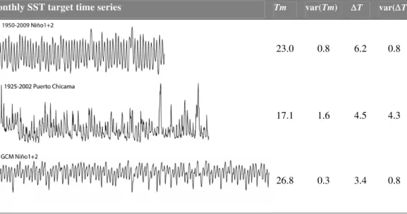
Table 2.Characteristics of monthly SST time series used as target in sensitivity experiments.

Only the first 100 yr of the GCM Ni ˜no1₊2 SST time series are shown.

Monthly SST target time series Tm var(Tm) ΔT var(ΔT)

23.0 0.8 6.2 0.8

17.1 1.6 4.5 4.3

26.8 0.3 3.4 0.8

(28)

CPD

7, 2477–2510, 2011

M. Carr ´e et al.

Title Page

Tables Figures

◭ ◮

Back Close

Full Screen / Esc

Discussion

P

a

per

|

Dis

cussion

P

a

per

|

Discussion

P

a

per

|

Discussio

n

P

a

per

|

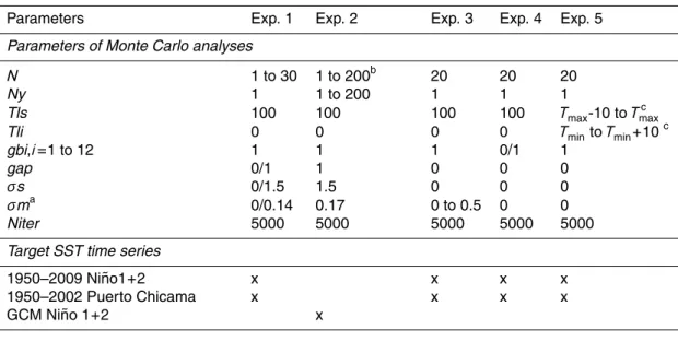
Table 3.Parameter setting in sensitivity experiments 1 to 5. Gray cells indicate varying param-eters.

Parameters Exp. 1 Exp. 2 Exp. 3 Exp. 4 Exp. 5

Parameters of Monte Carlo analyses

N 1 to 30 1 to 200b 20 20 20

Ny 1 1 to 200 1 1 1

Tls 100 100 100 100 Tmax-10 toT

c max

Tli 0 0 0 0 TmintoTmin+10

c

gbi,i=1 to 12 1 1 1 0/1 1

gap 0/1 1 0 0 0

σs 0/1.5 1.5 0 0 0

σma 0/0.14 0.17 0 to 0.5 0 0

Niter 5000 5000 5000 5000 5000

Target SST time series

1950–2009 Ni ˜no1+2 x x x x

1950–2002 Puerto Chicama x x x x

GCM Ni ˜no 1+2 x

a_σ_m2

=σa2+σw2+σc2.

b_N

·Ny=200. c

(29)

CPD

7, 2477–2510, 2011

M. Carr ´e et al.

Title Page

Tables Figures

◭ ◮

Back Close

Full Screen / Esc

Discussion

P

a

per

|

Dis

cussion

P

a

per

|

Discussion

P

a

per

|

Discussio

n

P

a

per

Random sampling Monthly SST

time series

sample i of N monthly SST windows

Signal perturbation

sample i of N surrogate proxy records

T_m0 var(T_m0)

∆T0 var(∆T₀) C0 =

T_mi var(Tmi)

∆T_i var(∆Ti) C_i=

[Ei = Ci - C0]i=1, 5000 5000 iterations

Systematic Error = <Ei>i=1, 5000 Standard Error = σ(E_i)_{i=1, 5000}

Potential systematic Error Calibration dataset (Tj, Pj)

Proxy model, T=f(P)

(30)

CPD

7, 2477–2510, 2011

M. Carr ´e et al.

Title Page Abstract Introduction Conclusions References Tables Figures ◭ ◮ ◭ ◮ Back Close

Full Screen / Esc

Printer-friendly Version Interactive Discussion Discussion P a per | Dis cussion P a per | Discussion P a per | Discussio n P a per |

0 10 20 30 21

22 23 24 25

0 10 20 30 21

22 23 24 25

0 10 20 30 21

22 23 24 25

0 10 20 30 21

22 23 24 25

0 10 20 30 0

2 4 6

0 10 20 30 0

0.5 1 1.5

0 10 20 30 0

0.5 1 1.5

0 10 20 30 0

2 4 6

0 10 20 30 5

6 7 8

0 10 20 30 5

6 7 8

0 10 20 30 5

6 7 8

0 10 20 30 5

6 7 8

0 10 20 30 -1

0 1 2 3

0 10 20 30 -1 0 1 2 3 4

0 10 20 30 -1

0 1 2 3

0 10 20 30 -1 0 1 2 3 4

noise σc noise σm noise gap=1,2 noises σc, σm, and gap=2

Tm

Var(Tm)

∆T

Var(∆T)

N N N N

Fig. 2. Results of experiment 1 with the 1950–2009 Ni ˜no1+2 SST time series. Mean values

ofTm, var(Tm),∆T, and var(∆T) (black bold lines) calculated from 5000 iterations of surrogate

proxy simulations (MoCo algorithm), and compared to the expected values (green) of the target time series, versus the sample size (e.g. number of shells). Systematic errors are indicated

by the difference between the mean calculated value and the expected value. Dotted lines

show the standard error interval (_±1σ) for an ideal proxy (no signal perturbation) versus the

sample size. Thin black lines show the standard error interval (_±1σ) for surrogate proxies

with stochastic noise. In the first three columns, the effects of spatial variability (σs), monthly

variability (σm), and the occurrence of random growth breaks (blue: 1 per year, black:2 per