Abstract— Optimization of design parameters based on electromagnetic simulation of microwave circuits is a time-consuming and iterative procedure. To provide a fast and accurate frequency response for a given case study, this paper employs a neural network modelling approach. First, one of the case study's outputs, i.e., scattering parameter (|S21|) in dB, is predicted using a
neural network model. Then the particle swarm optimization is employed to optimize the design parameters. The proposed method in designing the filter compares with two others methods for a case study. The simulation results show the capability of the proposed method in designing an optimized filter in a proper time.
Index Terms— neural networks, Microwave structures, particle swarm optimization, modelling.
I. INTRODUCTION
Neural networks are information processing systems inspired by the human brain’s ability to learn
from observations [1]. Neural networks are efficient alternatives to conventional methods, such as
numerical modelling methods which could be computationally expensive, or analytical methods
which could be difficult to obtain, or empirical models whose range and accuracy could be limited.
Due to their ability and adaptability to learn, generalizability, fast real-time operation, and ease of
implementation, they have been used in microwave design problems, RF, and microwave
computer-aided design problems [2].
In microwave applications, a neural network can train to mimic the electrical behavior of the
circuit. Then, it can be used in high-level simulation and design, providing a fast response to the
learned task [3], [4]. Moreover, neural networks can be employed along with evolutionary algorithms
such as genetic algorithm [5] and particle swarm optimization [6] to optimize the system under study.
In this application, a neuarl network can use with an electromagnetic packages, such as HFSS, CST,
ADS, to optimize the design.
In this paper, to accelerate the frequency sweep required in the full-wave simulators,for calculating
the S-parameters of a double folded stub microstrip filter, an artificial neural network is employed.
The neural network is trained, by achieved patterns from an electromagnetic package, to approximate
the S-parameters in the region of interest. The proposed model has capability to perform the frequency
Optimal Design of Double Folded Stub Microstrip
Filter by Neural Network Modelling and Particle
Swarm Optimization
Amir Banookh, S. Masoud Barakati
sweep fast and accurate, in comparison with the available electromagnetic packages. To optimize the
designed model the particle swarm optimization method is used.
The neural network structure is explained in the next section. Section 3 is dedicated to describe the
of particle swarm optimization. The case study is introduced in section 4. To verify the proposed
model, simulation results are illustrated in section 5. The last section is conclusions.
II. THE STRUCTURE OF NEURAL NETWORK
In this section, the structure of neural networks and its ability to model the behavior of RF and
microwave components are described.
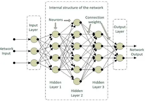
The MLP is a commonly used neural network structure, in which the neurons are grouped into
layers. The MLP contains input, hidden, and output layers. Each layer consists of some nodes and
fully connected to the next one. Node (or neuron) is a processing element with a nonlinear activation
function. The activation functions are applied to the weighted sum of the inputs of a neuron to
produce the output. Fig. 1 shows the structure of MLP neural network; consist of one input layer,
three hidden layers, and one output layer.
Fig. 1. Structure of the MLP artificial neural networ
Input neurons receive stimulus from outside the network, while the output of output neurons are
externally used. Hidden neurons receive stimulus from some neurons and their outputs are stimulus
for some other neurons. Different neural networks can be constructed by using different types of
neurons and by connecting them in different configurations [8].
The weights are the most important factor in determining the MLP function. Training is the act of
presenting the network with some sample data and modifying the weights to better approximate the
desired function. The weighting parameters, which are real numbers, are initialized before training the
MLP. During training, they are updated iteratively in a systematic manner. Typically many iterations
backpropagation learning technique can be used. The basic backpropagation algorithm is based on
minimizing the error of the network using the derivatives of the error function. Most common
measure of error is the mean square error: E = (target – output)2. Partial derivatives of the error with
respect to the weights:
Output Neurons: ∂E/∂wji = -outputiδj, (1)
where δj = f’(netj) (targetj – outputj), and j = output neuron, i = neuron in last hidden
Hidden Neurons: ∂E/∂wji = -outputiδj, (2)
where δj = f’(netj) Σ(δkwkj), j = hidden neuron, i = neuron in previous layer k = neuron in next layer.
Calculation of the derivatives flows backwards through the hidden and input layers of the network.
These derivatives point in the direction of the maximum increase of the error function. A small step
(learning rate) in the opposite direction will result in the maximum decrease of the (local) error
function:
wnew = wold – α∂E/∂wold , (3)
where αis the learning rate.
Once the neural network training is completed, the weighting parameters remain fixed throughout
the usage of the neural network as a model.
The case-study is modeled by a multilayer perceptron (MLP) neural network simulated in a
MATLAB environment [7].
III. PARTICLE SWARM OPTIMIZATION
In this section, a brief description of particle swarm optimization (PSO) is presented. PSO is a
stochastic optimization technique [9]-[16], that was developed in 1995 by Eberhart and Kennedy. It is
a global optimization algorithm, which can effectively be used to solve multidimensional optimization
problems [17]. PSO attempts to simulate the swarming behavior of birds, bees, fish, etc. It aims at
increasing the probability of encountering global extremum points without performing a
comprehensive search of the entire search space. PSO can easily be implemented and its performance
is comparable to other stochastic optimization technique, such as genetic algorithm and simulated
annealing [14].
The PSO starts with an initial population of individuals, which are named swarm of particles. Each
particle in the swarm is randomly assigned an initial position and velocity. The position of the particle
is an N-dimensional vector, representing a possible set of optimization parameters. Each particle starts
from its initial position, xi=[xi1,xi2,...,xin]T, and its initial velocity, vi =[vi1,vi2,...,vin]T. According
to the individual and the swarm experience, the velocity and position of each particle are updated
during the algorithm search. The goodness of a new particle position, a possible solution, is measured
by evaluating a fitness function. The process of updating velocities and positions continues by the
time that one of the particles in the swarm finds the position with best fitness. Since the particles will
The main steps of PSO algorithm can be summarized as follows:
A. Definition of the solution space
In this step, the minimum and maximum values for each dimension in the N-dimensional
optimization problem are specified.
B. Definition of the fitness function
The fitness function is a problem-dependent parameter which is used to evaluate and measure the
goodness of a position representing a valid solution.
C. Random initialization of the swarm positions and velocities
The position and velocity of the particles are randomly initialized. For faster convergence, however,
it is preferred that they are randomly chosen from the solution space. The number of particles is
problem-dependent, and for most engineering problems a swarm size of thirty particles is good
enough [18]. To complete the initialization step, the initial position of each particle is labeled as the
particle’s best position, Pbest. Also, the position of the particle with best fitness among the whole
swarm is labeled as the global best position, Gbest. The word ‘best’ means highest or lowest
depending on whether the problem is a minimization or maximization problem.
D. Updating the velocity and position of a particle
In this step, the following sub-steps are carried out for each particle
• Velocity update
The velocity of the ith particle in the jth dimension, vij is updated according to (4)
, ..., , 2 , 1 )), ( ( )) ( ( ) ( ) 1
(t wv t c1r1 Pbest x t c2r2 Gbest x t j N
vij + = ij + ij − ij + j − ij = (4)
where xij represents the position of the ith particle in the jth dimension. The time index of the current
and previous iterations are denoted by ‘t+1’ and ‘t’, respectively. r1 and r2 are two random numbers in
range [0–1], generated by uniformly distributed random functions. The parameters c1 and c2 are the
relative weight of the personal best position and the relative weight of the global best position,
respectively. Both c1 and c2 are typically chosen in range [0-2] [17]. The parameter w, which is called
the “inertial weight”, is a number in the range [0–1]. It specifies the weight by which the particle’s
current velocity depends on its previous velocity. The references [19]-[26] proposed a method on
selecting and optimizing the PSO parameters.
• Position update
The position of the ith particle in the jthdimension is updated according to the following equation
. ..., , 2 , 1 ), 1 ( ) ( ) 1
(t x t v t j N
xij + = ij + ij + = (5)
• Fitness evaluation
First, the fitness of the updated N-dimension position in the previous step is evaluated. If the
a new Pbest. Also, if the returning number is better than the fitness corresponding to the Gbest, the
updated N-dimension position is labeled as a new Gbest.
E. Checking the termination criterion
The algorithm may be terminated if the number of iterations reaches a pre-specified maximum
number of iterations or the fitness corresponding to the Gbest is close enough to a desired number. If
none of these conditions is satisfied, the algorithm will return to the previous step.
IV. CASE-STUDY: DOUBLE FOLDED STUB MICROSTRIP FILTER
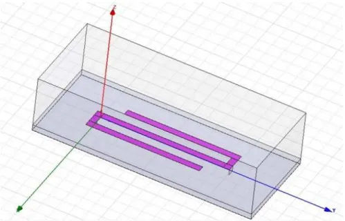
The structure of Double Folded Stub Microstrip filter in High Frequency Simulation Software
(HFSS) is shown in figure. 2. It is made of a perfect conductor on the top of a Duroid substrate with a
relative dielectric constant of 9.9 and a height of 5 mil, and the bottom layer is made with a perfect
conductor ground plane. The two design variable parameters are S and L2 and three other design
parameters, w1 , w2 , and L1 are fixed at 4.8, 4.8, and 93.7 mil, respectively. The diagram of Double
Folded Stub Microstrip filter, that shows the design parameters, is illustrated in figure 3. To represent
such input–output relationship, an artificial neural network model is trained for given design
parameters within the region of interest. The neural network model is used to provide a fast estimation
of |S21| based on given filter’s geometrical parameters.
Consider x, y, and w vectors refer to the neural network input, output, and weighting parameters,
respectively. The neural network input-output relationship is given by
). , (x w f
y = (6)
The neural network input is given by
[
sL2]
T,x = ω (7)
where ω is a range of frequency. The sample points are generated using an electromagnetic simulator,
i.e., HFSS [27]. The region of interest, in mil, is 3.6 ≤S≤ 7.6 and 80.3 ≤L2≤ 100.3. The objective of
training is to adjust neural network weighting parameters, such that the neural model output best
match to the output data of HFSS simulation.
Fig. 2. Structure of Double Folded Stub Microstrip filter in HFSS software
Fig. 3. Diagram of Double Folded Stub Microstrip filter
V. SIMULATION RESULTS
A. The Neural Network training using HFSS output data
As mentioned in previous section, an MLP neural network trained based on HFSS output pattern to
approximate the |S21| parameters in the region of interest. The neural network model will perform the
frequency sweep fast and accurate in comparison with HFSS.
The neural network consists of one input, one hidden, and one output layer. The input, hidden, and
output layers contain of three neurons, 40 neurons, and one neuron, respectively. The hidden and
output layer transfer functions are hyperbolic tangent sigmoid and linear functions, respectively. The
41 input vectors x, in form of equation (7) and in uniformly distributed sample points, are used as
training patterns. The traing algorithm is performed using a bach mode and Levenberg-Marquardt
method [7],[8]. During the trainnig algorithm the validation and testing of the results are very
important to obtain a well-generalised MLP without overtraining [7], [28]. The trainig data will be
model. Proper division of the data is controlled by checking the plots of test and validation errors, at
the same time [28]. If test and validation error plots do not demonstrate similar characteristics, this is
an indication of poorly divided data. In this study, the input data is devided into three sets, randomly,
as: 60% for traing, 20% for validation, and 20% for performance test. The learning rate, maximum
number of epoch, and maximum mean square error are set to 0.1, 1000, 0.0001, respectively. Figure 4
shows the training, validation, and testing errors versus number of epochs (iterations) for the MLP in
the case study. The training algorithm terminates if the validation error increases (after six sequence
iterations), or the limitations of maximum error/epoch are exceeded. As illustrated in Figure 4 the
training algorithm is terminated in 246 epochs (because of validation error), while the training error is
small enough (0.000166), and the test and validation error show similar characteristics.
Fig. 4. The training, validation, and testing errors versus number of epochs (iterations) for the MLP
After training stage, the neural network model is evaluated based on 40 sample points.
The |S21| parameter of Double Folded Stub Microstrip filter is simulated by HFSS package and
proposed neural network model for three different filters. The simulation results are depicted in figure
5, where two models are compared. As shown in the figure, the models responses are fairly close.
Therefore, the trained neural network output can use instead of HFSS response. This replacing helps
Fig. 5. S21 frequency responses of HFSS and the Neural Network models for three different filters
B. Optimization the design parameters using PSO technique
To find the optimal values of the physical parameters, the PSO technique, introduced in section 3, is
adopted. To optimize the double folded stub filter of figure 2, the following design specifications are
considered.
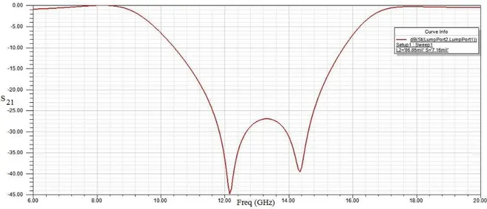
I) S21 ≥ -3dB for ƒ≤9.5 GHz and ƒ≥16.5 GHz,
II) S21 ≤ -25dB for 12 GHz≤ ƒ ≤ 14GHz.
The number of particles and total number of iterations in PSO are 80 and 100, respectively. Other
PSO parameters are c1=1, c2=2, and w=0.9.
The optimal parameters given by PSO are: S=7.16 mil and L2=86.85 mil.
Fig. 6. Response of the Double Folded Stub Microstrip filter for optimal parameters
Table I compares three design methods for the case study, i.e., using HFSS package, using HFSS
combined with PSO, and the proposed method. Substituting the trained neural network with HFSS
package speeds up finding the optimal parameters of the filter. The running time of the simulated
proposed method, using a machine with CPU Corei7 1.73GHz and 4G RAM, takes about 17 minutes,
while using a direct PSO method in HFSS (where the number of particles and the total number of
iterations in PSO are 80 and 100, and HFSS runs 8000 times) it takes about 3466 minutes, i.e., 208
times slower than the proposed method. In addition, the proposed method obtains the optimal design
parameter, and the HFSS package and PSO can be linked in MATLAB, instantaneously.
Table I. comparison the proposed method with two tools for finding the optimal parameters of the filter
Design approach Electromagnetic
Package (HFSS) HFSS-PSO
HFSS-ANN-PSO (Proposed method)
Design and optimization are
linked - NO Yes
Running Time
(for the case study) Very slow 3466 mins 17 mins
Conclusion
To optimal design of |S21| parameter of a Double Folded Stub Microstrip filter using an
electromagnetic package, such as, HFSS, is a time consuming method. Although, the optimal
parameter of the filter can be obtained by an optimization method, the HFSS package and the
optimization method cannot link together easily. In this paper, an MLP neural network, trained based
on the HFSS responses, is adopted for the fast and accurate calculation of |S21| parameter of the filter.
The trained neural network model has capability of providing an accurate frequency response in a
fraction of a second. In addition, to optimize the designed filter based on the neural network response,
a particle swarm optimization (PSO) method is employed to achieve the optimal parameter. The
trained MLP and PSO algorithm are interfaced in MATLAB, while for finding the optimal response
using the HFSS package, an optimization algorithm should be executed off-line. Based on the
simulation results for a case study, the proposed method is 208 times faster than using HFSS package.
Therefore, it can conclude that the proposed method is a fast and accurse tools for designing a Double
Folded Stub Microstrip filter.
REFERENCES
[1] Q. J. Zhang and K. C. Gupta, Neural Networks for RF and Microwave Design, Norwood, MA: Artech House, 2000.
[2] Q. J. Zhang and K. C. Gupta, “Neural Networks for RF and Microwave Design- From Theory to Practice,”IEEETransactions on Microwave Theory and Techniques, vol. 51, April 2003.
[3] K. C. Gupta, “Emerging trends in millimeter-wave CAD,” IEEETransactions on Microwave Theory and Techniques, vol. 46, pp. 747–755, June 1998.
[4] V. K. Devabhaktuni, M. Yagoub, Y. Fang, J. Xu, and Q. J. Zhang,“Neural networks for microwave modeling: Model development issues and nonlinear modeling techniques,” International Journal of RF MicrowaveComputer-Aided Engineering, vol. 11, pp. 4–21, 2001.
[5] S. N. Sivanandam and S. N. Deepa, Introduction to Genetic Algorithms, Springer, 2010.
[6] M. Clerc, Particle Swarm Optimization, John Wiley & Sons, 2010.
[7] MATLAB, version 7.11.0.584 (R2010b), The MathWorks Inc., 2010.
[8] F. Wang, V. K. Devabhaktuni, C. Xi, and Q. J. Zhang, “Neural network structures and training algorithms for microwave applications,” International Journal of RF Microwave Computer-Aided Engineering, vol. 9,pp. 216–240, 1999.
[9] R.C. Eberhart& J. Kennedy, A new optimizer using particle swarm theory, Proc. Sixth International Symposium on Micromachine and Human Science, Nagoya, Japan, 1995, 39–43.
[10] J. Kennedy & R.C. Eberhart, Particle swarm optimization, Proc. IEEE International Conference on Neural Networks, Piscataway, NJ, 1995, 1942–1948.
[12] J. Kennedy, R.C. Eberhart, & Y. Shi, Swarm intelligence (San Francisco: Morgan Kaufmann Publishers, 2001).
[13] J. Kennedy & R. Mendes, Population structure and particle swarm performance, on Proc. Congress Evolutionary Computation (CEC 02), vol. 2, 2002, 1671–1676.
[14] J. Kennedy & J.M. Spears, Matching algorithms to problems: An experimental test of the particle swarm and some genetic algorithms on the multimodal problem generator, Proc. IEEE World Congress Computational Intelligence Evolutionary Computation, 1998, 78–83.
[15] S. Tavakoli and A. Banookh, Robust PI Control Design Using Particle Swarm Optimization, Journal of Computer Science and Engineering, vol 1, issue 1, p36-41, 2010
[16] M. Zeinadini, S. Tavakoli and A. Banookh, Modelling and Design of Microwave Structures Using Neural Networks and Particle Swarm Optimization, Journal of Telecommunication, vol 3, issue 1, 2010.
[17] R.C. Eberhart& Y. Shi, Evolving artificial neural networks, Proc. Int. Conf. Neural Networks Brain, Beijing, P.R.C., 1998.
[18] J. Robinson & Y. Rahmat-Samii, Particle swarm optimization in electromagnetics, IEEE Transactions on Antennas and Propagation, 52(2), 2004, 397–402.
[19] I.C. Trelea, The particle swarm optimization algorithm: Convergence analysis and parameter selection, Information Processing Letters, 85, 2003, 317–325.
[20] M. Clerc and J. Kennedy, The particle swarm—explosion, stability, and convergence in a multidimensional complex space, IEEE Transactions on Evolutionary Computation, 6(2), 2002, 58–73.
[21] A.I. El-Gallad, M.E. El-Hawary, A.A. Sallam, & A. Kalas, Enhancing the particle swarm optimizer via proper parameters selection, Canadian Conference on Electrical and Computer Engineering, 2002, 792–797.
[22] D. Bratton and T. Blackwell, A Simplified Recombinant PSO, Journal of Artificial Evolution and Applications, 2008.
[23] Y. Shi & R. Eberhart, A modified particle swarm optimizer, Proc. IEEE World Congr. Computational Intelligence Evolutionary Computation, 1998, 69–73.
[24] Y. Shi & R. Eberhart, Empirical study of particle swarm optimization, Proc. Congr. Evolutionary Computation (CEC 99), vol. 3, 1999, 1945–1950.
[25] F. van den Bergh & A.P. Engelbrecht, Effects of swarm size on cooperative particle swarm optimizers, Proc. Genetic and Evolutionary Computation Conference 2001, San Francisco, USA, 2001.
[26] G. Evers, An Automatic Regrouping Mechanism to Deal with Stagnation in Particle Swarm Optimization, Master's thesis The University of Texas - Pan American, Department of Electrical Engineering, USA, 2009.
[27] Ansoft High Frequency Structure Simulator (HFSS), ver. 12.1, Ansoft Corporation, Pittsburgh, PA, 2009.