Abstract— The optimal design of a set of two permanent magnet generators that share the same cross section to reduce the manufacturing cost is presented using a gradient optimization algorithm. The optimization tool is used to define the optimal number of pole pairs of the set of machines and the optimal permanent magnets width respecting the geometrical and performance constraints. The design is validated using a FEM analysis tool.
Index Terms—Optimization, design, permanent magnet generator, magnetic circuits design, set optimization.
I. INTRODUCTION
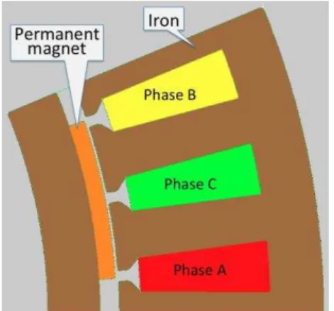
The case study presented here concerns the design of two generators with surface permanent
magnets with different speed and power, which have the same cross section in both stator and rotor
(Fig. 1). One of them is rated 3kW and 350rpm and is intended for rooftop wind turbines, whereas the
other is rated 4kW and 500rpm and is intended for mini hydropower plants, both with 220V
phase-to-phase voltage. For the purposes of the project, both feed on a resistive load. Sharing the same
cross-section aims to reduce the cost of stamping tools and stock of components (mainly magnets).
The objective of the optimal design is to find a design respecting, what we call, the M Main Input
Specifications (MIS) concerning the rated speeds, powers and voltage. Minimizing total material cost
Ctmat of both structures and restraining efficiency η must be achieved by respecting those
specifications. The external diameter of the stator must also be less than or equal to 300mm.
The originality of the paper is to propose a generic methodology, using optimization, for making
simultaneously the design of two devices sharing some components like typically the same cross
section of iron or the same magnet.
II. THE SIZING AND OPTIMIZATION MODELS BASIS
The methodology presented here uses an optimization approach for which we introduce the concept
of sizing model, and optimization model.
The sizing model will be used for finding a first design for one machine (we can call this design,
design A)
Then an optimization model is introduced for making the simultaneous optimization of the two
machines sharing the same cross-section.
Let us begin presenting the basis of the two models used in our design:
Optimal design of a set of permanent magnet
generators with the same cross
-
section
Renato Carlson, Frederic Wurtz,
UTFPR Ponta Grossa-Parana Brazil [email protected],
the sizing model for finding an initial design which is only an estimation, and not an optimal
solution
the optimization model that will allow us not only to optimize the design, but also to make
simultaneously the design of two machines sharing the same cross section.
A. The Sizing Model used for making the initial non optimal design of one machine
First we have to remember that the goal of the design is, starting from the M main input
specifications, to find at least one set of machines characterized by:
N design parameters (DPi): this set includes the construction parameters of the device like the
geometrical ones along with parameters such as the winding and the length of the machine.
K performances (Perfk): this set includes physical characteristics of the machines (with
parameters like torque and currents) as well as physical constraints (with parameters like
current density and inductions).
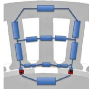
Fig. 1. The Permanent Magnet Generator (PMG) structure.
In practice, the problem is quite complex as, in general, we have N>>M. So a “good” sizing model needs to offer an efficient way to calculate those N design parameters starting from only the M main input specifications. In a “good” sizing model, this is obtained thanks to the designer knowledge that allows fixing the values of a subset of N1 design parameters and the values of a subset of K1
performances.
The remaining (N−N1) design parameters and (K-K1) performances are calculated through a mixture of knowledge, physics, and expertise.
The sizing model is purely analytical and is built based mainly on these references [1,2].
To compute the N design parameters and K performances of the device, the sizing model takes as
input:
M=5 main input specifications (nA = 350 rpm, PnA = 3 kW, nB = 500 rpm, PnB = 4 kW,
Vn = 220V) that are defined by the requirements of the application.
N1=12 initial design parameters on some geometric and design parameters (pole pairs p, stack
length Lstk, etc.) that are defined by the designer experience for the given application.
induction Bd, the current density J, etc.) that are also defined by the designer experience for the
given application.
To give a value to the following:
N-N1 remaining “design parameters”, that are mainly dimensions and winding characteristics,
and
K-K1 “performances”, like torque, efficiency, resistances and reactances,
NbE equations are defined as follows:
(1)
Among the NbE equations, we typically have the following:
Analytical equations that allow calculating some design parameters from some “options on performances”;
Heuristic and statistic equations.
The advantages of sizing models are as follows:
They are able to find a design starting from the M main input specification parameters: this the
key point and the main characteristic of a sizing model,
They can make the design with a simple calculation owing to the use of analytical knowledge
[1,2],
Owing to the heuristic knowledge they contain, they are able to directly provide a good initial
solution for calculating all the N design parameters and K performances based on just N1 “design parameters” and K1 “performances”.
The limits of the sizing model are as follows:
The precision, that is well adapted for making a very good initial design, is too low for
optimizing the design precisely;
This precision is difficult to improve because these models have to retain the property to be
inverse models: the price for being able to calculate the majority of the design parameters
starting from the M minimal specifications, and a limited number N1 of “design parameters” and of K1 “performances” means necessarily making assumptions and approximations;
They do not provide an optimal solution because assumptions have been made especially on the
N1 initial design parameters and K1 initial performances. So we do not have an idea of the
global design space and the possible optimal solutions;
They rely heavily on the knowledge and experience of the designer.
It is also difficult to take into account the following:
The important constraints on the design: typically in this case Des ≤ 300 mm; for this, complex
iterations may be needed manually because Des is one of the N-N1 output design parameters of
the SM of our PMG,
the efficiency η.
For this, again, complex iterations by hand are needed. Besides, because the model has been made
with heuristics and simplification, it does not contain sufficient information for making a precise
optimization. Especially, the main difficulty here is, if we were able to build a sizing model for one
machine, it is more difficult to build a sizing model for making the simultaneous design of two
machines sharing a same component, like the cross section. For this the solution is to have an
optimization model associated to an optimization methodology.
B. The concept of optimization modelfor making the simultaneous design of two machines sharing components
1) The optimization model for the sizing of single machine
We will first introduce what a sizing model is for the sizing by optimization of a stand-alone device.
An Optimization Model is a direct model: this means that this model is written in the natural
physical way or in the natural direct sense.
This has two consequences:
1°. This model can be more complicated, with less assumptions and hypotheses. Thus we can use
more sophisticated approaches like reluctances network that allow to model phenomena like
saturation of flux leakages (phenomena that are usually neglected in a sizing model).
Typically with such a model, the induction of the airgap will become an output of the model,
calculated by the reluctance network (an not an input parameter for which the designer will
have to guess a value).
2°. Usually in such a model, not all the M Main Input Specifications (MISj) are inputs of the
model.
Consequently, this OM will have as inputs the following:
M2 “main input specification”,
N2 "input design parameters,”
K2 “input performances,”
to give a value to the following:
M-M2 “main input specification,”
N−N2 remaining “design parameters,”
K-K2 “performances.”
Finally, an OM links Ip input parameters (with p ∈[1,M2+N2+K2]) to Oo outputs parameters (with
o∈[1,M-M2+N-N2+K-K2]).
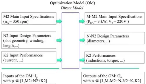
Thus, in an OM, the main key point is that all the “main input specifications” are not necessarily inputs; for our set of PMGs, only nA = 350 rpm and remain as inputs, whereas PnA and Vn are outputs.
The OM developed for one machine verifies N2 + K2 = 26 (with parameters about geometry,
current density, rated power, torque etc.) are output parameters. The structure of an OM for sizing a
single machine is illustrated on figure 2.
Fig. 2. Structure of an optimization model for a single machine.
Making the design with this kind of model is a complex task because some of the M main
specifications that we have to reach are outputs of the model (typically, PnA and Vn for our PMG). To
solve this problem, the OM should be coupled with an optimization algorithm what will be explained
latter in this paper.
2) The optimization model for the sizing of two machines sharing components
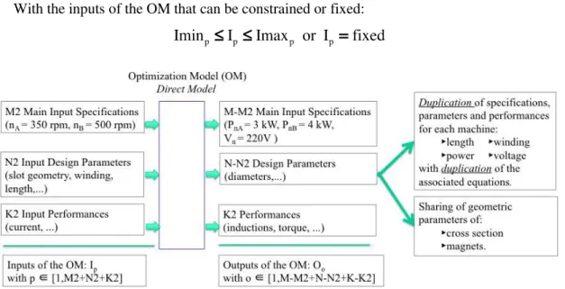
The structure of an OM for sizing two machines sharing components is illustrated on figure 3. The
main principle is:
Duplication of specifications, parameters and performances specific to each machines, with
duplication of the associated equations,
but sharing of parameters linked to the common components: typical the geometrical
parameters linked to the common cross section (height and length of tooth, height of rotor and stator yoke, …).
The consequence of this is that this OM model, adapted for making the simultaneous design of two
machines is necessarily more complex, with more parameters.
III. THE PROPOSED OPTIMIZATION METHODOLOGY FOR MAKING THE SIMULTANEOUS DESIGN OF TWO MACHINES SHARING COMPONENTS:
In this paper we propose to use of the OM with an optimization algorithm able to solve the
following generic problem:
Minimizing an objective function that is one of the outputs of our OM:
(2)
or (3)
With the inputs of the OM that can be constrained or fixed:
(4)
Fig. 3. The new optimization model for optimizing 2 machines sharing componentes (cross section plus magnets)
This allows us to solve the design problem by being able to limit any parameter to a fixed value or
constrain it inside an interval regardless of whether this parameter is an input or an output. Therefore,
for our PMGs, there is no problem in configuring the solution such that nA = 350 rpm, PnA = 3 kW,
nB = 500 rpm, PnB = 4 kW, Vn = 220V and Des ≤ 300 mm even if those parameters are output
parameters of our OM.
From a theoretical and practical point of view, the difficulty is that the number of inputs and outputs
can be quite high, especially when we want to make the simultaneous design of several machines
sharing components, since the number of parameters will increase with this number of machines and
this even if some parameters are shared.
That is why we propose here to use the methodology described in [3] and implemented in the
CADES software [4]. This methodology is particularly efficient for solving optimization problems of
electromagnetic devices with a high number of input and output parameters and constraints.
The principle is:
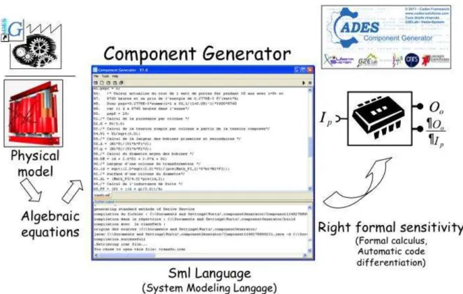
1° The designer has to give the model as a “white box” to a generator (a kind of compiler). “White box” means that the designer will give all the algebraic equations of the model of the device in a declarative language (called in CADES the SML language for System Modeling
Language). Then the generator, thanks to an automated process, creates a code that computes
the model. Moreover, as the generator produces computation code, it also obtains the
derivatives of the equations and produces the sensitivity computation code. This has been done
with sophisticated approaches likes symbolic computation, or Automatic Code Differentiation.
This produces a software component, able to compute all the equations Oo(Ip) but also all the
partial derivatives (or Jacobian) as illustrated on Figure 1. By this way it generates the right
easily large optimization problems (with a high number of input and output parameters).
Fig. 4. The “white box” approach used for optimization – compilation of the model and formal computation of the sensitivity
2° The Optimizer module using the model and its right formal sensitivity does the optimization.
Thanks to the fact that we have the computation of the formal right sensitivity, and that we have
use deterministic optimization algorithms like Sequential Quadratic Programming [5] With this
approach With this approach], we have then an optimization process that is very quick (only a
few seconds), even with a high number of parameters and constraints. This property is very
important for making simultaneous optimization of several machines. Figure 5 gives an
overview of this optimizer available in the CADES software.
With this approach, the OM can be analytical but also semi-numerical. For instance, for the OM of
our set of PMGs, we use a reluctance network [6] (see Fig. 6) approach to compute the induction in
the air gap, the stator, and the rotor for each optimization step. This reluctance network is realized
using the software RELUCTOOL that is part of the CADES optimization tool. It takes into account
the magnetic saturation of the iron during the optimization process. The reluctance network was
validated comparing the magnetic induction in the air-gap with that obtained using the finite elements
method.
Fig. 6. PMG no-load reluctance magnetic equivalent circuit.
The OM being analytical or semi-analytical the best performances are obtained, it evaluates quickly
and it is quite easy to compute derivatives that will greatly improve the efficiency of optimization
algorithms. This is why, for us, a purely numerical model is not a good OM; it has to be considered as
a validation model, to be used after the optimization process to verify the result.
Lastly, we can say that many works and papers have proposed solutions for optimization of
electromagnetic devices. We can think about [7-9] and commercial solutions are of course available.
The originality of this paper is to propose an approach for making optimization with models with a
high number of parameters and constraints, what is a necessity for making simultaneous optimization
of devices sharing components. We have validated this methodology for reaching this goal, a good
strategy is to develop semi-analytical models, which can be derived in a formal way and linked to a
deterministic algorithms.
Because the OM is written in a physically direct sense, the designer has no limits for including
equations or additional submodels (for instance, a thermal model) depending on the design
parameters and conditions of use, and with more physical information.
IV. AGENERAL DESIGN PROCESS USING THE COMPLEMENTARY PROPERTIES OF THE SIZING AND OPTIMIZATION MODELS
Here, we will describe the complete optimal design process in three steps using the sizing model
and the optimization model successively.
A. Step 1: Preliminary Sizing
In this step, the SM of part II is used. It can be implemented in tools like Excel or Mathcad. Here,
we are able to compute an initial design starting only from M = 3 main input specifications. The total
cost of material of the 3 kW / 350 rpm generator for this design is US$ 813 and has an efficiency of
B. Step 2: Optimization in continuous sizing space
In this step, the OM of Section III is used with the methodology and software described in [3,4].
Here, a continuous optimization process is carried out with the following characteristics for the
3 kW / 350 rpm generator:
The optimization process is carried out with a gradient optimization algorithm (sequential
quadratic programming [3]). Because the entire sensitivity of the optimization is computed [4],
this results in a very fast optimization process, only a few seconds for our PMG.
This optimization is made for the first time by letting all the parameters vary continuously.
The optimization algorithm needs an initial starting point; the machine of the preliminary sizing
(Step 1) is used.
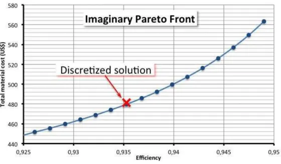
For our PMG, this allows us to make a mono-objective optimization in which we minimize the total
material as a function of the efficiency. This consists of an entire set of optimizations, where we
discretize the efficiency to several values between 92.5% and 95%, and for each discrete value of
efficiency in this range, we make an optimization in which we minimize the material cost. This allows
building the curve showed in Figure 7. This curve corresponds to the Pareto Front in the continuous
space (what we call the imaginary Pareto front: IPF [10]). This curve represents the best possible
compromise between cost and efficiency in the continuous space. We talk about imaginary machines,
as many of the PMG of this front cannot directly be built. This is because some continuous parameters
need to be discretized (like the number of conductors in a slot).
Fig. 7. The optimal design graph.
However, the advantage of this curve is that it is very fast to compute (only in a few seconds for our
PMG) and gives the theoretical limit of the best possible compromise between cost and efficiency.
We can see from Fig. 7 that the optimization procedure led us to a much lower total material cost.
Although the initial sizing gave us a starting point very far from the optimal design graph, the OM
find acceptable, Ctmat remains under US$ 560, representing an important cost reduction compared with
what we obtained with the SM. Ctmat can be as low as US$ 480 if we accept a 93.5% efficiency.
C. Step 3: Discretization
In Step 2, all the optimal designs (the machines of the IPF front) are made in the continuous space.
We need to design at least one machine by discretizing the parameters that must be discretized
(typically, for our PMG, the number of conductors in a slot must be an integer and the diameter of the
wires must be chosen from a commercial round wires table). For this, we use the OM with a simple
procedure: a successive rounding of continuous parameters to the nearest discrete values, and we
restart optimization after each discretization. Of course, a more sophisticated procedure can be
imagined, but this one is sufficient for our PMG to obtain a machine that is very close to the one
obtained in step 2 as can be seen in Fig. 8 where a red cross marks this solution.
V. OPTIMAL DESIGN OF THE SET OF TWO MACHINES
Once the OM is established, we now have to adjust it to consider the two PMG.
This is not difficult because the main dimensions are defined to be the same. The only dimension
that is allowed to be different between the two machines is the length of the stack. Also, the stator
winding is allowed to be different between the two machines, which means that the number of
conductors in the slots and the section of the wire will be different. A one slot per pole per phase
winding is chosen to simplify the design in a first moment.
1) Defining the number of pole pairs
We start the optimal design by choosing the number of pole pairs of the two machines. To do that,
we used the optimization tool CADES with the Pareto tool for calculating the set of two imaginary
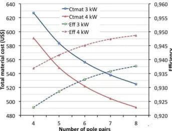
machines for different numbers of pole pairs. Fig. 8 shows that the total material cost decreases when
the number of pole pairs increases. Note: in all cases the outer stator diameter is limited to 300 mm
and the optimizations always push it to this maximum, as expected. We verify also in this figure that
the efficiency increases with the number of pairs of poles and the higher efficiency of the 4 kW/500
rpm machine due to its lower copper losses.
The variation of the cost of copper, iron and magnets with the number of pole pairs is shown in
Fig. 9 for the 3 kW/350 rpm machine as well as for the 4 kW/500 rpm machine. We observe here that
the higher cost corresponds to the NdFeB permanent magnets, as expected. We observe from this
figure that the larger percentage cost reduction corresponds to copper.
The main limitation considered in choosing the number of pole pairs of the two machines was
related to the width of stator yoke and teeth. Considering the external diameter of the two machines,
that was fixed to 300 mm maximum, and for reason of mechanical rigidity we decided to limit the
stator yoke and teeth width to 10 mm corresponding to 6 pole pairs for both machines. Fig. 10.a
shows the detail of the slots and teeth for three pole pair numbers (in the same scale) that allows
the tooth and yoke width as the pole pair number increases.
Fig. 8. Total material cost and efficiency versus the number of pole pairs.
Fig. 9. Cu, Fe, and Nd.FeB cost as a function of the number of pole pairs.
(a) (b)
Fig. 10. (a) Detail of the slots for three different number of poles; (b) Tooth and yoke width as a function of the number of pole pairs.
2) Defining the magnets thickness
Having determined the number of pairs of poles, we now define the proper thickness of the
permanent magnets examining how this dimension affects the total material cost, the efficiency and
As a design criterion we adopted a permeance coefficient for the permanent magnets equal to 10,
meaning that the air gap is 1/10 of the permanent magnets thickness [1].
To do that, once again, we used the optimization tool CADES with the Pareto tool for calculating
the set of two imaginary machines for different permanent magnets thicknesses [5].
Considering the high cost of the NdFeB permanent magnets it is important to consider this aspect in
defining its thickness. Fig. 11.a shows that after 4 mm the total cost increase presents a kind of
saturation with the permanent magnet thickness.
On the other side, a beneficial effect of increasing the permanent magnet thickness is to increase the
efficiency. This can be seen in Fig. 11.b where we find that the efficiency of the 3 kW machine is
lower than that of the 4 kW machine. This difference of efficiency, although the two machines are
designed with the same current density, is due to the greater resistance per phase of the 3 kW
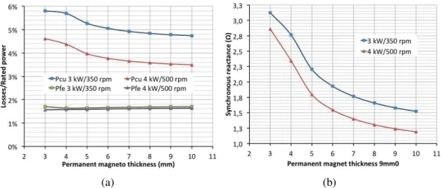
machine. This is corroborated by the copper losses, shown in Fig. 12.a, which are larger in the 3 kW
machine, while the iron losses are much smaller than the copper losses and are fairly similar on both
machines.
(a) (b) Fig. 11. (a) Total material cost as a function of the permanent magnet thickness,
(b) Efficiency as a function of the permanent magnets thickness.
Another aspect to be considered is the armature reaction, which was found to require some
attention. We will discuss this phenomenon later, but it should be noted here that a lower synchronous
reactance is desired. Fig. 12.b shows that the synchronous reactance is strongly influenced by the
thickness of the permanent magnets as expected.
Considering all these aspects we decided to adopt a 5 mm thickness for the permanent magnets of
both machines.
VI. VALIDATIONOFTHEDESIGN
Since the optimization model is an analytical, or semi analytical model, a verification of the optimal
design produced must be made. This can be done efficiently by using a finite element model. Here,
we used the EFCAD software as a validation model considering the 6 pole pairs 3 kW /350 rpm PMG
(a) (b)
Fig. 12. (a) Losses and (b) synchronous reactance as a function of the permanent magnet thickness.
Fig. 13 shows the no-load magnetic flux density distribution over the machine cross section. The
permanent magnets used in the design are NdFeB with a remanent flux density of 1.21 T. This figure
shows that the flux densities defined in the project (see Table I) are achieved.
Fig. 13. No-load magnetic flux density distribution.
The main input specifications of the 3 kW/350 rpm generator that will be checked are the
phase-to-phase voltage, the electromagnetic torque and the load power. To verify these specifications we used a
module of EFCAD that connects the finite elements model to an external three-phase resistive load,
star connected. This is a time varying simulation at fixed speed; hence steady state results are attained
Fig. 14. Full load steady-state magnetic field distribution.
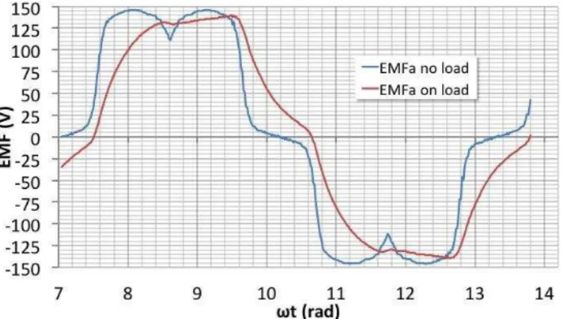
The phase-to-neutral EMF of the 3 kW PMG is shown in Fig. 15. In this figure we can see the
effect of the armature reaction over the phase-to-neutral EMF.
Fig. 15. Phase-to-neutral EMF: at no-load and on load conditions.
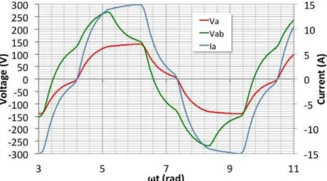
Fig. 16 shows the phase-to neutral and phase-to-phase load voltage and the phase current. The
amplitude of the first harmonic of the current is 15.5 A and that of the phase-to-phase voltage is
250 V. Hence we obtained a phase-to-phase voltage that is 13.6% higher than the specified. This is
due to the difficulty of properly taking into account the effects of the armature reaction in the design.
The other specification concerns the rated torque of 88.56 N.m. Fig. 16 show the instantaneous
electromagnetic torque of the 3 kW/350 rpm machine. We can see in this figure the effect of the
saturation of the magnetic circuit over the instantaneous torque, reducing the average torque from
97.3 N.m under linear conditions to 92.2 N.m under saturated conditions. The rated torque is a little
lower than that value. This figure also shows the effect of skewing the rotor magnets, significantly
reducing the torque ripple. This would be the result of continuously skewing the permanent magnets
of 9 mechanical degrees or 9/10 of the stator slot pitch. As this is not feasible in practice, the rotor
Fig. 15. Load voltage (phase-to-neutral and phase-to-phase) and current.
Fig. 16. Electromagnetic torque.
VII. CONCLUSIONS
The design of a set of two permanent magnet generators was performed using the CADES
optimization tool. The optimal number of pole pairs and the magnet thickness were obtained using
the same tool with a Pareto tool that enabled to make the parameters variation very effectively. A
FEM analysis tool that couples the field calculation to an external electrical circuit in the time domain
verified the design results. The results show a good agreement between the design and the FEM
simulation. The modeling of the armature reaction is still a complicated task that is being studied. A
prototype was built that will serve to corroborate the simulation by experimental tests.
REFERENCES
[1] J.R. Hendershot Jr and T.J.E. Miller, Design of Brushless Permanent- Magnet Machines, Oxford, Motor Design Books, LLC, 2010.
[2] J. Pyrhönen, T. Jokinen and V. Hrabovcová, Design of Rotating Electrical Machines”. New York, John Wiley & Sons, 2009.
[3] F. Wurtz, J. Bigeon and C. Poirson, “A methodology and a tool for the computer aided design with constraints of electrical devices,” IEEE Trans. on Magn., vol 32, no 3, pp 1429-32, May 1996
[4] B. Delinchant et al. "An Optimizer using the Software Component Paradigm for the Optimization of Engineering Systems", COMPEL: The Int. Journal for Comp. and Math. Electrical and Electronics Eng.”, Vol. 26, No. 2, pp. 368 -379, 2007.
[6] B. Du Peloux, L. Gerbaud, F. Wurtz, V. Leconte, F. Dorshner, “Automatic generation of sizing static models based on reluctance networks for the optimization of electromagnetic devices“, IEEE Transactions on Magnetics, Vol. 42, Issue 4, April 2006, pp. 715 – 718.
[7] O. Mohammed, D. A. Lowther, M. H. Lean, and B. Alhalabi: On the creation of a generalized design optimization environment for electromagnetic devices, IEEE Trans. on Magn, vol.37, pp.3562-3565, 2001.
[8] O. Mohammed, S. Liu, and Z. Liu: Physical modeling of electric machines for motor drive system simulation, IEEE PES Conference, pp.781-786, 2004.
[9] R. Ramarathnam, B.G. Desai, V. Subba Rao, "A comparative study of minimization techniques for optimization of induction motor design", IEEE Trans. on PAS, Vol. PAS 92, No 5, pp. 1448-1454, Sep./Oct. 1973.
[10]F. Wurtz, P. Kuo-Peng and E. S. De Carvalho, “The Imaginary Pareto Front: a helpful Tool for setting Optimization Problem”, COMPUMAG 2011 Conference, Sydney, Australia.