www.atmos-chem-phys.net/16/9089/2016/ doi:10.5194/acp-16-9089-2016
© Author(s) 2016. CC Attribution 3.0 License.
Can we detect regional methane anomalies? A comparison between
three observing systems
Cindy Cressot1, Isabelle Pison1, Peter J. Rayner2, Philippe Bousquet1, Audrey Fortems-Cheiney1, and Frédéric Chevallier1
1Laboratoire des Sciences du Climat et de l’Environnement, CEA/CNRS/UVSQ, Gif-sur-Yvette, France 2School of Earth Sciences, University of Melbourne, Melbourne, Australia
Correspondence to:Isabelle Pison ([email protected])
Received: 17 March 2016 – Published in Atmos. Chem. Phys. Discuss.: 18 March 2016 Revised: 17 June 201 – Accepted: 5 July 2016 – Published: 25 July 2016
Abstract. A Bayesian inversion system is used to evaluate the capability of the current global surface network and of the space-borne GOSAT/TANSO-FTS and IASI instruments to quantify surface flux anomalies of methane at various spatial (global, semi-hemispheric and regional) and time (seasonal, yearly, 3-yearly) scales. The evaluation is based on a signal-to-noise ratio analysis, the signal being the methane fluxes inferred from the surface-based inversion from 2000 to 2011 and the noise (i.e., precision) of each of the three observing systems being computed from the Bayesian equation. At the global and semi-hemispheric scales, all observing systems detect flux anomalies at most of the tested timescales. At the regional scale, some seasonal flux anomalies are detected by the three observing systems, but year-to-year anomalies and longer-term trends are only poorly detected. Moreover, reli-ably detected regions depend on the reference surface-based inversion used as the signal. Indeed, tropical flux inter-annual variability, for instance, can be attributed mostly to Africa in the reference inversion or spread between tropical regions in Africa and America. Our results show that inter-annual anal-yses of methane emissions inferred by atmospheric inver-sions should always include an uncertainty assessment and that the attribution of current trends in atmospheric methane to particular regions’ needs increased effort, for instance, gathering more observations (in the future) and improving transport models. At all scales, GOSAT generally shows the best performance of the three observing systems.
1 Introduction
nu-merical weather prediction (Desroziers et al., 2005) within a robust Monte Carlo approach to optimize the input er-ror covariance matrices of a global CH4 inversion system. Here, we use their results as a starting point to character-ize the uncertainty of the year-to-year variations of the in-ferred fluxes at various temporal (e.g., seasonal, annual, 3-yearly, monthly) and spatial (global, latitudinal bands, large regions) scales in order to document which anomaly sig-nals from the inversions are reliable and which are not re-liable within our framework. To do so, three different global CH4observation systems are considered: surface sites from various global networks (flasks and continuous), the space-borne Infrared Atmospheric Sounding Interferometer (IASI) that provides a middle-to-upper tropospheric column and the Thermal And Nearinfrared Sensor for carbon Observation -Fourier transform spectrometer (TANSO-FTS), that observes the total column from space. Using the flux anomalies of the surface inversion as the signal, signal-to-noise ratios for dif-ferent temporal and spatial scales are computed, the noise be-ing the uncertainty (precision) of the year-to-year changes of the inferred fluxes for each observing system. Signal-to-noise ratios are then considered as a statistical criterion to evaluate the ability of an observing system to retrieve the CH4 flux inter-annual variability.
The paper is structured as follows. The theoretical frame-work and the different data sets are presented in Sect. 2. The signal-to-noise ratios are presented in Sect. 3 and further dis-cussed in Sect. 4.
2 Method
2.1 Inversion framework
Our inversion system is based on a variational formulation of Bayes’ theorem, as detailed by Chevallier et al. (2005), which has been adapted to the inversion of CH4fluxes by Pi-son et al. (2009). It allows inferring grid-point-scale fluxes, thereby avoiding gross aggregation errors (Kaminski et al., 2001), while assimilating the large flow of satellite data at appropriate observation times and locations. It ingests obser-vations of CH4 mole fractions and prior information about the variables that are to be optimized, with associated error covariance matrices. Bayesian error statistics of the inferred variables are computed from a Monte Carlo ensemble of in-versions which is consistent with the assigned-prior and ob-servation errors (Chevallier et al., 2007). The inversion sys-tem includes the LMDZ transport model of Hourdin et al. (2006) at a resolution of 3.75◦×2.5◦(longitude by latitude) for 19 vertical levels nudged to ECMWF-analyzed winds in its on-line mode. Here, we use its off-line mode that exploits the output variables of the on-line version. We couple it to a simplified chemistry module to represent the interactions between CH4 and the hydroxyl radical (OH), its main sink in the atmosphere, and between methyl chloroform (MCF)
and OH. Note that the loss due to chlorine in the marine boundary layer is not implemented yet in this model. When it assimilates both CH4and MCF mole fractions, as is done here, it synergistically optimizes both CH4surface sources at weekly and model grid resolution and OH at weekly resolu-tion over four latitude bands (−90/−30,−30/0, 0/30, 30/90). This setup therefore dynamically distinguishes between CH4 net surface emissions (soil uptake included) and atmospheric loss. The system iteratively minimizes the Bayesian cost function (made nonquadratic by the nonlinear chemistry) us-ing the M1QN3 algorithm (Gilbert and Lemaréchal, 1989).
This system is applied here to assimilate data from each of three CH4 observing systems together with data from a MCF observing system (to constrain OH concentrations), in the configuration used by Cressot et al. (2014). The reader is referred to Cressot et al. (2014) for a detailed description of this configuration. It is important here to recall that the prior fluxes (fires excepted) have no inter-annual variability (IAV). This choice is made for IAV to be generated by atmospheric observations and atmospheric transport and chemistry and not by prior IAVs of emissions (and sinks) which are still uncertain or even controversial (e.g., Schaefer et al., 2016; Hausmann et al., 2016; Nisbet et al., 2014).
Two types of inversions are presented in this study: – a reference inversion (hereafter called REFSURF)
us-ing CH4and MCF surface measurements from Decem-ber 1999 to DecemDecem-ber 2011; and
– three ensembles of inversions (see Sect. 2.3 for the use of these), one using surface measurements only (called SURF hereafter), one using IASI data and MCF ob-servations only (called IASI hereafter) and one using TANSO-FTS data and MCF observations only (called GOSAT hereafter, from the name of the platform, Greenhouse Gases Observing Satellite); each ensemble consists of 10 1-year inversions from October 2009 to September 2010, with respective inversion setups tuned according to an objective analysis described in Cressot et al. (2014).
For all inversions, the minimization of the nonquadratic cost function is stopped when the ratio of the final to the ini-tial norm of the gradient is less than 0.01.
2.2 Data sets
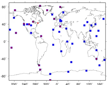
Figure 1.Surface sites from the NOAA, CSIRO, NIWA and EC networks used in this study with red circles for surface sites observ-ing MCF dry air mole fractions and blue squares for surface sites observing CH4dry air mole fractions.
et al., 1991). We also use station Alert (ALT) from Environ-ment Canada (EC) (Worthy et al., 2009). MCF measureEnviron-ments are provided by 11 NOAA surface sites (Montzka et al., 2011) and are used to constrain OH concentrations (Pison et al., 2009). The surface sites used in our inversions are pre-sented in Fig. 1.
We use observations of the middle-to-upper tropospheric CH4 column made by IASI, a thermal interferometer on-board the Meteorological Operational (MetOp) satellites. This quantity is retrieved based on a nonlinear inference scheme (Crevoisier et al., 2009) within 30◦ of the Equator over both land and ocean at about 09:30/21:30 LT, with an accuracy of 1.2 % (≈20 ppb).
Last, we use observations of the CH4 atmospheric total column over land from TANSO-FTS, a near-infrared spec-trometer onboard GOSAT. Total columns are retrieved by op-timal estimation using the algorithm of Parker et al. (2011) and with a precision of∼0.6 % (≈10 ppb).
The averaging kernel or weighting function and the prior profile (when available) of each IASI or TANSO-FTS re-trieval are directly accounted for in the inversion system fol-lowing Connor et al. (2008).
2.3 Error statistics
The error statistics are described in detail in Cressot et al. (2014). For the fluxes, the spatial correlations are defined bye-folding lengths of 500 km over land and 1000 km over ocean (no correlation between land and ocean); time corre-lations are defined by ane-folding length of 2 weeks. It was checked that these choices led to a budget uncertainty which is consistent with the uncertainty of bottom-up inventories as described in Kirschke et al. (2013).
The input error statistics for the prior and the observations are tuned using objective diagnostics as described by Cressot et al. (2014). This means that they exhibit some objectivity that is seen to translate into realistic Bayesian posterior er-ror statistics, which in particular make all present inversions statistically consistent at the annual and global or regional scales (Cressot et al., 2014).
In order to keep the computational burden to a reason-able level, we compute the posterior error statistics from a Monte Carlo inversion ensemble of 10 times 1 year for each of the three observing systems (ensembles GOSAT, IASI and SURF as described in Sect. 2.1).
The posterior error statistics (the “noise” for our study) are estimated as follows:
– We estimate the ratio of posterior-to-prior standard de-viations of the annual flux errorsr=σa
σb from the en-semble, a quantity which is more robust thanσaandσb individually for small ensembles (because some of the underspread affects the prior and the posterior in a sim-ilar way). The number of members in the ensemble de-pends on the timescale, e.g., 10 members for the yearly timescale (10 inversions, each one covering 1 year), 120 members for the monthly timescale.
– We estimate the posterior standard deviations of the an-nual flux errors by multiplyingrby the known value of σb, i.e., the one implied by our error covariance matrix (computed from the above assumptions).
– The posterior standard deviations of the multi-annual flux errors fornyears are obtained by applying a fac-tor of√1
nto the previous result, assuming that the errors are uncorrelated from one year to the next.
– The posterior standard deviations of the difference be-tween fluxes from one year to the next (i.e., the error on the IAV for 2 consecutive years) is computed by apply-ing an inflation factor of√2 to the previous result, still assuming that the errors are uncorrelated from one year to the next. We assume this approach to be a conserva-tive hypothesis since, in reality, some of the transport and retrieval errors are recurrent, thereby inducing pos-itive correlations and reducing the inflation factor. The variability of CH4concentrations depends on the ox-idizing capacity of the atmosphere, which is largely con-trolled by OH concentrations. Since OH concentrations are constrained through MCF data in our multi-species inversion system (Sect. 2.1), the uncertainty on OH (≈5 % after opti-mization) is accounted for in the uncertainty of the inferred CH4emissions and of their inter-annual variations.
Figure 2. Regions on the model grid, adapted to key areas for methane fluxes.
data, to their distribution in time and space and also to their sensitivity to methane surface fluxes and to their uncertainty. It may also depend on the ability of the transport model to properly represent the various data.
2.4 Evaluation criterion
CH4 regional flux anomalies are defined here as the devia-tion from a reference of the CH4inferred fluxes for various time periods, from the monthly to the 3-yearly scale. The reference is the 2004–2005 mean over the same time period. The aim of this definition is to get the order of magnitude of the year-to-year changes at various timescales. As the 2004– 2005 reference corresponds to a period of minimum atmo-spheric methane growth rate (Dlugokencky et al., 2011), it leads to more positive anomalies for the longer timescales. The regional scale is based on the regions defined and shown in Fig. 2 and large latitudinal bands are defined as BorN for latitudes higher than 60◦N, MidN between 30 and 60◦N, TropN between 0 and 30◦N, TropS between 0 and 30◦S, MidS between 30 and 60◦S and BorS higher than 60◦S. We study various spatial and temporal scales of inferred flux anomalies.
Our criterion consists in evaluating the ability of the ob-serving systems to detect CH4anomalies of a given ampli-tude, defined by the reference inversion. For this, we define a signal-to-noise ratio:
– The inversion with surface measurements is chosen to provide the signal as the data cover a long time window (2000–2011) as compared to the two other observing systems. This longer window makes it possible to sam-ple the CH4 IAV more robustly than a 2–3-year sion. We assume that the fluxes inferred by this inver-sion are representative of state-of-the art inverinver-sions cur-rently published. The signal is actually the CH4 anoma-lies for the various timescales derived from REFSURF. – For the three observing systems (SURF, IASI and
GOSAT), the Bayesian posterior errors of the
year-to-year changes of CH4fluxes, computed from the Monte Carlo ensemble as described in Sect. 2.3, constitute the noise associated to each observing system.
Finally, the criterion for detecting CH4anomalies is that the signal-to-noise ratio is larger than 1 (≈68 % confidence).
Comparing signal-to-noise ratios amounts to comparing noises normalized by the expected signals. The normaliza-tion provides an absolute criterion to assess the timescales and regions at which the CH4anomalies are reliable. How-ever, the quality of the chosen signal remains debatable and our diagnostic for GOSAT and IASI may be pessimistic in areas where SURF signal-to-noise ratio is low.
In the following, the presentation of the results is done for three timescales (seasonal, yearly and 3-yearly trends) before assessing their sensitivity to temporal and spatial aggrega-tions.
3 Results: signal-to-noise ratios 3.1 Seasonal-scale detection
The signal-to-noise ratios are computed over 3-month peri-ods (JFM, AMJ, JAS and OND, hereafter referred to as sea-sons for simplicity) from 2000 to 2011, i.e., 48 occurrences (12 JFM, 12 AMJ, 12 JAS and 12 OND).
The three observing systems are able to detect almost all anomalies at the global scale (Table 1). As expected, the frac-tion of detected anomalies decreases with the spatial scale. At the global scale, 91–93 % of the flux anomalies are de-tected depending on the observing system (Table 1). At semi-hemispheric scales (excluding MidS and BorS areas), this range is 0–87 % (median=49.5 %), GOSAT having the best range (8–87 %) compared to IASI (12–60 %) and SURF (0– 66 %). The lack of detection in MidS and BorS is not signif-icant considering the small methane fluxes involved. At the regional scale, the detection range is 0–79 % (median=4%), with large contrasts. Again the range is more favorable for GOSAT (0–79 %, median=7 %) than for SURF (0–75 %, median=3 %) and IASI (0–72 %, median=0 %). Anoma-lies in the USA, Central America (CentralAm), temperate Africa (SouthernAfr), Middle East, and Australia and New Zealand (AustrNZ) are not detected by any of the three serving systems. GOSAT is the only one of the three ob-serving systems to detect any anomaly in temperate South America (SouthSAm) and northern Africa (NorthAfrWest, NorthAfrEast).
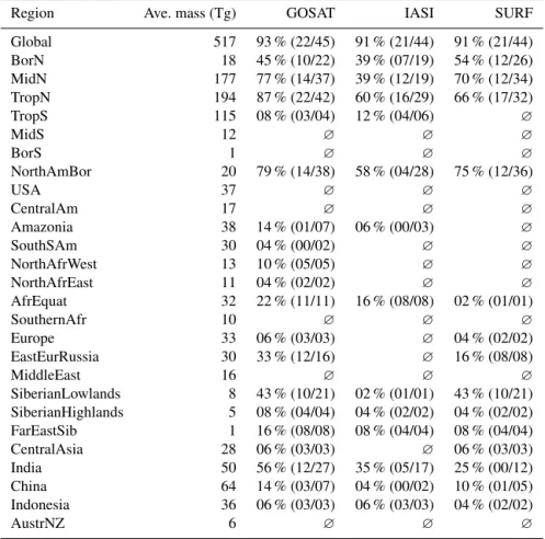
(Ta-Table 1.Detection of the signal consisting in the anomalies at the seasonal timescale, i.e., quarters of the year (JFM, AMJ, JAS, OND). The signal is the difference between each quarter in the 2000–2011 period (i.e., 48 occurrences) and the 2004–2005 average from REFSURF. The noise is computed at the quarter timescale from each of the three observation systems, GOSAT, IASI and SURF. See Sects. 2.4 and 2.3 for details. In each cell of the table, we showX% (Y Y /ZZ) whereX% is the percentage of quarterly anomalies detected (among 48 possible), Y Yis the number of positive anomalies detected among theZZdetected anomalies. Column labeled Ave. mass indicates the average emitted mass of CH4over 2004–2005 in the area.
Region Ave. mass (Tg) GOSAT IASI SURF
Global 517 93 % (22/45) 91 % (21/44) 91 % (21/44)
BorN 18 45 % (10/22) 39 % (07/19) 54 % (12/26)
MidN 177 77 % (14/37) 39 % (12/19) 70 % (12/34)
TropN 194 87 % (22/42) 60 % (16/29) 66 % (17/32)
TropS 115 08 % (03/04) 12 % (04/06) ∅
MidS 12 ∅ ∅ ∅
BorS 1 ∅ ∅ ∅
NorthAmBor 20 79 % (14/38) 58 % (04/28) 75 % (12/36)
USA 37 ∅ ∅ ∅
CentralAm 17 ∅ ∅ ∅
Amazonia 38 14 % (01/07) 06 % (00/03) ∅
SouthSAm 30 04 % (00/02) ∅ ∅
NorthAfrWest 13 10 % (05/05) ∅ ∅
NorthAfrEast 11 04 % (02/02) ∅ ∅
AfrEquat 32 22 % (11/11) 16 % (08/08) 02 % (01/01)
SouthernAfr 10 ∅ ∅ ∅
Europe 33 06 % (03/03) ∅ 04 % (02/02)
EastEurRussia 30 33 % (12/16) ∅ 16 % (08/08)
MiddleEast 16 ∅ ∅ ∅
SiberianLowlands 8 43 % (10/21) 02 % (01/01) 43 % (10/21) SiberianHighlands 5 08 % (04/04) 04 % (02/02) 04 % (02/02) FarEastSib 1 16 % (08/08) 08 % (04/04) 08 % (04/04)
CentralAsia 28 06 % (03/03) ∅ 06 % (03/03)
India 50 56 % (12/27) 35 % (05/17) 25 % (00/12)
China 64 14 % (03/07) 04 % (00/02) 10 % (01/05)
Indonesia 36 06 % (03/03) 06 % (03/03) 04 % (02/02)
AustrNZ 6 ∅ ∅ ∅
ble 1), but in contrast to the other regions and to the other timescales, the prior error statistics already lead to detection rates of 58 % for the prior. This shows that the tropical IASI soundings do not add information for this region and at this timescale, as expected. GOSAT performs better by detect-ing more than three-quarters of the anomalies, about one-third of which are in winter (Fig. 3, due to almost null emis-sions when the surface is snow-covered), one-third in sum-mer and one-third in fall (Fig. 3, due to maximum emissions in summer). Due to a larger noise (≈1.5 Tg vs. ≈1.2 Tg for GOSAT, Fig. 4a), SURF misses all springs (Fig. 3). In the larger BorN area, only winter and summer are detected (Fig. 3).
In the tropics, some areas also have large seasonal vari-ations, mainly due to biomass burning or rice-paddies. In AfrEquat, some of the AMJ positive signals generated are detected by GOSAT and IASI (Fig. 4a). Note that SURF per-forms poorly in this area (Table 1) due to the lack of sta-tions, which leads to large noise (≈3.3 Tg, Fig. 4a). In
In-dia and China, rice-paddy practices led to a seasonal cycle of methane emissions with a maximum in JAS and a mini-mum in JFM (Matthews et al., 1991). The three systems de-tect anomalies in JFM and JAS (Fig. 3) with consistent signs (≈half positive, half negative anomalies) for GOSAT, neg-ative anomalies preferentially detected by IASI and SURF (Table 1).
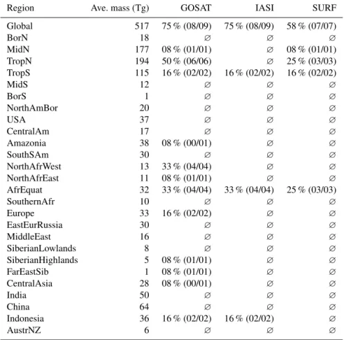
3.2 Yearly-scale detection
Figure 3.Number of detected seasons over the 12 possible for winter (JFM, blue), spring (AMJ, green), summer (JAS, red) and fall (OND, orange) in the various regions.
with a median of 0 %; the only regions above 25 % of de-tection are tropical Africa (AfrEquat) and NorthAfrWest for GOSAT. No detection is obtained in key regions for methane emissions such as Amazonia (except GOSAT at 8 %), India, China and North America (NorthAmBor, USA).
The differences between the three observing systems are larger at the yearly scale than at the seasonal scale: GOSAT and IASI detect 75 % of the 12 possible global occurrences vs. 58 % for SURF (Table 2). At the regional scale, GOSAT
Figure 4.Noise at the seasonal timescale by the three observing systems (bars) and box plots (median, 25 and 75 %) for the signal in various areas (latitudinal bands and regions). Detection is achieved when the signal is larger than the noise, i.e., for all the occurrences in each box plot which lay outside the matching colored bar.
In agreement with the intuition of Bergamaschi et al. (2013) that performing gross averages makes it possible to extract a signal from the inversion, the detection is enhanced in the latitudinal bands, e.g., detection rates ≥25 % in TropN for GOSAT and SURF. But it remains difficult to robustly extract yearly flux anomalies. Therefore, we now focus our analy-sis on longer timescales, with a longer time aggregation of 3 years, to get hints at the longer trends in methane emissions.
3.3 Trend detection over 2000–2011
To study the detection of flux long-term trend over 12 years, a compromise has to be found between the rather short length of this time window and the time aggregation of fluxes, which needs to filter out year-to-year changes. Aggregating through time while still retaining a small-enough resolution to discuss trends over 2000–2011, we define four time win-dows of 3 years each: 2000–2002, 2003–2005, 2006–2008 and 2009–2011. The reference period for the definition of the anomalies of each of these four periods is still 2004–2005 (Sect. 2.4).
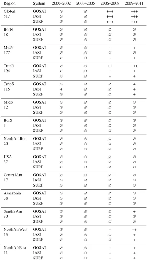
At the global scale, the emissions have slowly decreased from 2000 to 2005, with a global minimum in 2004–2005, then increased at a larger rate after 2006 (Kirschke et al., 2013). The three observing systems are able to detect the large positive anomalies after 2006 and detect nothing before (Table 3). The three observing systems are able to detect the same temporal evolution of the signal in TropN and TropS. Only GOSAT and SURF detect MidN anomalies; the lower detection by IASI at these latitudes is expected since the data used here are only within±30◦of the Equator (Table A1, no IASI data in MidN). The signal in BorN is never detected.
This is consistent with the recent increase of methane global emissions coming mostly from the tropics and to a lesser ex-tent from the northern midlatitudes, as suggested by Berga-maschi et al. (2013) and Nisbet et al. (2014).
Being able to detect anomalies at a smaller spatial scale could help attributing the changes in methane emissions to particular processes. Unfortunately, even when aggregating 3 years together (instead of 1 year as in Sect. 3.2), it is still difficult to detect regional anomalies.
Table 2.Detection of the signal consisting in the anomalies at the yearly timescale. The signal is the difference between each year in the 2000–2011 period (i.e., 12 occurrences) and the 2004–2005 average from REFSURF. The noise is computed at the yearly timescale from each of the three observation systems, GOSAT, IASI and SURF. See Sects. 2.4 and 2.3 for details. In each cell of the table, we showX% (Y Y /ZZ) whereX% is the percentage of yearly anomalies detected (among 12 possible),Y Yis the number of positive anomalies detected among theZZdetected anomalies. Column labeled Ave. mass indicates the average emitted mass of CH4over 2004–2005 in the area.
Region Ave. mass (Tg) GOSAT IASI SURF
Global 517 75 % (08/09) 75 % (08/09) 58 % (07/07)
BorN 18 ∅ ∅ ∅
MidN 177 08 % (01/01) ∅ 08 % (01/01)
TropN 194 50 % (06/06) ∅ 25 % (03/03)
TropS 115 16 % (02/02) 16 % (02/02) 16 % (02/02)
MidS 12 ∅ ∅ ∅
BorS 1 ∅ ∅ ∅
NorthAmBor 20 ∅ ∅ ∅
USA 37 ∅ ∅ ∅
CentralAm 17 ∅ ∅ ∅
Amazonia 38 08 % (00/01) ∅ ∅
SouthSAm 30 ∅ ∅ ∅
NorthAfrWest 13 33 % (04/04) ∅ ∅
NorthAfrEast 11 08 % (01/01) ∅ ∅
AfrEquat 32 33 % (04/04) 33 % (04/04) 25 % (03/03)
SouthernAfr 10 ∅ ∅ ∅
Europe 33 16 % (02/02) ∅ ∅
EastEurRussia 30 ∅ ∅ ∅
MiddleEast 16 ∅ ∅ ∅
SiberianLowlands 8 ∅ ∅ ∅
SiberianHighlands 5 08 % (01/01) ∅ ∅
FarEastSib 1 08 % (01/01) ∅ ∅
CentralAsia 28 08 % (00/01) ∅ ∅
India 50 ∅ ∅ ∅
China 64 ∅ ∅ ∅
Indonesia 36 16 % (02/02) 16 % (02/02) ∅
AustrNZ 6 ∅ ∅ ∅
the associated large fires, such as those experienced in 1997– 1998 or more recently in 2015–2016, for instance (National Weather Service – Climate Prediction Center, 2016).
Among the key areas for methane emissions, signals in Amazonia (dominated by tropical wetlands) and in BorN, particularly in SiberianLowlands (dominated by boreal wet-lands in summer), remain undetectable by the three sys-tems. In SiberianLowlands, the noises of the three systems are small (between 3.8 and 7.8 Tg (not shown)); in Ama-zonia, the noises of the satellites are relatively small (≈6 and≈7 Tg, respectively, for GOSAT and IASI), whereas the noise of SURF, for which no stations are available closer than ASC in the Atlantic, is ≈24 Tg (Fig. 7, 3Y case). Never-theless, all these anomalies remain smaller than the smaller noise, and are therefore not detectable in our framework. This is because the signal variability remains small after inversion (less than 20 % of the average mass over 2004–2005). Pos-sible reasons for this are an actual low variability in these regions for this period and the fact that the choice to limit IAV in the prior emissions to biomass burning together with
the lack of constraints from the atmosphere led the inferred fluxes to stick to the low IAV prior.
3.4 Detection at other timescales
Table 3.Detection of the signal consisting in the anomalies at the 3-yearly timescale. The signal is the difference between each 3-year time window in the 2000–2011 period (2000–2002, 2003–2005, 2006–2008, 2009–2011) and the 2004–2005 average from REFSURF. The noise is computed at the 3-yearly timescale from each of the three observation systems, GOSAT, IASI and SURF. See Sects. 2.4 and 2.3 for details. In each cell of the table, we show whether a positive anomaly, a negative anomaly or no anomaly is detected and with which signal-to-noise ratio: positive anomaly detected: +++=stn ratio>3, ++=stn ratio>2 and +=stn ratio>1; negative anomaly detected with−− =stn ratio<−2,− =stn ratio<−2,∅,=no anomaly detected. The number below the name of the area is the average emitted mass of CH4over 2004–2005 in the area.
Region System 2000–2002 2003–2005 2006–2008 2009–2011
Global GOSAT ∅ ∅ +++ +++
517 IASI ∅ ∅ +++ +++
SURF ∅ ∅ +++ +++
BorN GOSAT ∅ ∅ ∅ ∅
18 IASI ∅ ∅ ∅ ∅
SURF ∅ ∅ ∅ ∅
MidN GOSAT ∅ ∅ + +
177 IASI ∅ ∅ ∅ ∅
SURF ∅ ∅ + +
TropN GOSAT ∅ ∅ ++ +++
194 IASI ∅ ∅ + +
SURF ∅ ∅ + +
TropS GOSAT ∅ ∅ ∅ +
115 IASI + ∅ ∅ +
SURF ∅ ∅ ∅ +
MidS GOSAT ∅ ∅ ∅ ∅
12 IASI ∅ ∅ ∅ ∅
SURF ∅ ∅ ∅ ∅
BorS GOSAT ∅ ∅ ∅ ∅
1 IASI ∅ ∅ ∅ ∅
SURF ∅ ∅ ∅ ∅
NorthAmBor GOSAT ∅ ∅ ∅ ∅
20 IASI ∅ ∅ ∅ ∅
SURF ∅ ∅ ∅ ∅
USA GOSAT ∅ ∅ ∅ ∅
37 IASI ∅ ∅ ∅ ∅
SURF ∅ ∅ ∅ ∅
CentralAm GOSAT ∅ ∅ ∅ ∅
17 IASI ∅ ∅ ∅ ∅
SURF ∅ ∅ ∅ ∅
Amazonia GOSAT ∅ ∅ ∅ ∅
38 IASI ∅ ∅ ∅ ∅
SURF ∅ ∅ ∅ ∅
SouthSAm GOSAT ∅ ∅ ∅ +
30 IASI ∅ ∅ ∅ ∅
SURF ∅ ∅ ∅ ∅
NorthAfrWest GOSAT ∅ ∅ + ++
13 IASI ∅ ∅ ∅ +
SURF ∅ ∅ ∅ +
NorthAfrEast GOSAT ∅ ∅ + +
11 IASI ∅ ∅ + +
Table 3.Continued.
Region System 2000–2002 2003–2005 2006–2008 2009–2011
AfrEquat GOSAT ∅ ++ +++
32 IASI ∅ ∅ ++ +++
SURF ∅ ∅ + ++
SouthernAfr GOSAT ∅ ∅ ∅ ∅
10 IASI ∅ ∅ ∅ ∅
SURF ∅ ∅ ∅ ∅
Europe GOSAT + ∅ ∅ ∅
33 IASI ∅ ∅ ∅ ∅
SURF + ∅ ∅ ∅
EastEurRussia GOSAT ∅ ∅ ∅ ∅
30 IASI ∅ ∅ ∅ ∅
SURF ∅ ∅ ∅ ∅
MiddleEast GOSAT − ∅ ∅ +
16 IASI ∅ ∅ ∅ ∅
SURF ∅ ∅ ∅ ∅
SiberianLowlands GOSAT ∅ ∅ ∅ ∅
8 IASI ∅ ∅ ∅ ∅
SURF ∅ ∅ ∅ ∅
SiberianHighlands GOSAT ∅ ∅ ∅ ∅
5 IASI ∅ ∅ ∅ ∅
SURF ∅ ∅ ∅ ∅
FarEastSib GOSAT + ∅ ∅ ∅
1 IASI ∅ ∅ ∅ ∅
SURF ∅ ∅ ∅ ∅
CentralAsia GOSAT − ∅ ∅ ∅
28 IASI ∅ ∅ ∅ ∅
SURF ∅ ∅ ∅ ∅
India GOSAT ∅ ∅ ∅ ∅
50 IASI ∅ ∅ ∅ ∅
SURF ∅ ∅ ∅ ∅
China GOSAT ∅ ∅ ∅ ∅
64 IASI − ∅ ∅ ∅
SURF ∅ ∅ ∅ ∅
Indonesia GOSAT + ∅ ∅ ∅
36 IASI + ∅ + ∅
SURF ∅ ∅ ∅ ∅
AustrNZ GOSAT ∅ ∅ ∅ ∅
6 IASI ∅ ∅ ∅ ∅
SURF ∅ ∅ ∅ ∅
In key region Amazonia (Fig. 7), no signal is detected at the 3-yearly timescale nor at the monthly timescale by any of the three systems; only GOSAT detects about 8 % of the anomalies at the yearly timescale. Actually, the timescale at which the best detection rates are found depends on the re-gion and varies from the largest possible (3-year scale) to the 2-month scale. In Africa (NorthAfrWest, NorthAfrEast,
Figure 5.Impact of temporal aggregation on noise (bars) and sig-nal (box plots with median, 25 and 75 %) over 3-year time windows. Detection is achieved when the signal is larger than the noise, i.e., for all the occurrences in each box plot which lay outside the match-ing colored bar. Link to Table 3: the Global lines of the table corre-sponds to the 3Y bars here.
Figure 6.Impact of temporal aggregation on noise (bars) and sig-nal (box plots with median, 25 and 75 %) over 3-year time windows. Detection is achieved when the signal is larger than the noise, i.e., for all the occurrences in each box plot which lay outside the match-ing colored bar. Link to Table 3: the TropN lines of the table corre-sponds to the 3Y bars here.
At high latitudes (NorthAmBor), the best detection rates are found at the 2-monthly (SURF), 3-monthly (IASI) and 4-monthly (GOSAT) timescales (with 88–100 % for GOSAT, up to 75 % for IASI (but which is not better than the prior de-tection rate, see Sect. 3.1) and up to 77 % for SURF), which is consistent with seasonal cycles with a large magnitude over a short period of time in this region.
In order to further understand the various levels of detec-tion described above, we investigate the sensitivity of our re-sults to two main parameters of our setup: spatial aggregation and signal used.
4 Sensitivity analysis
4.1 Impact of spatial aggregation on trend detection Our inversion system solves for methane fluxes at model res-olution (3.75◦×2.5◦) worldwide. Although spatial and tem-poral correlations are prescribed (see Sect. 2.3), flux anoma-lies of different signs may still be obtained. These anomaanoma-lies may be either the realistic result of the constraints or due to the optimization taking an easy path when too few
con-Figure 7.Impact of temporal aggregation on noise (bars) and sig-nal (box plots with median, 25 and 75 %) over 3-year time windows. Detection is achieved when the signal is larger than the noise, i.e., for all the occurrences in each box plot which lay outside the match-ing colored bar. Link to Table 3: the Amazonia lines of the table corresponds to the 3Y bars here.
straints are available. The definition of larger areas may lead to summing up anomalies of opposite signs and hide (real-istic or not) spatial variations. We try here to investigate the impact of the spatial aggregation of model pixels in the case of one illustrative region, Amazonia, which is a key area for methane emissions and remains poorly detected by all the studied observing systems at all timescales (see Sect. 3.4). In the region, as defined on our model grid, the signal at the pixel scale is indeed patchy (Fig. 8). Dipoles of nega-tive/positive signal are summed up when aggregating at re-gional scale. The impact of the progressive aggregation of rings of pixels from the center of Amazonia is displayed in Fig. 9 for the 3-yearly timescale; the signal is detected by all systems for the four 3-year periods up to the third ring, i.e., for a region covering 25 pixels instead of 66. It would then be possible to define the regions based on the spatial aggregation that allows the best detection rates for the chosen observing system. Nevertheless, this may be inconsistent with users’ needs, e.g., if they are expressed in terms of country-based budgets.
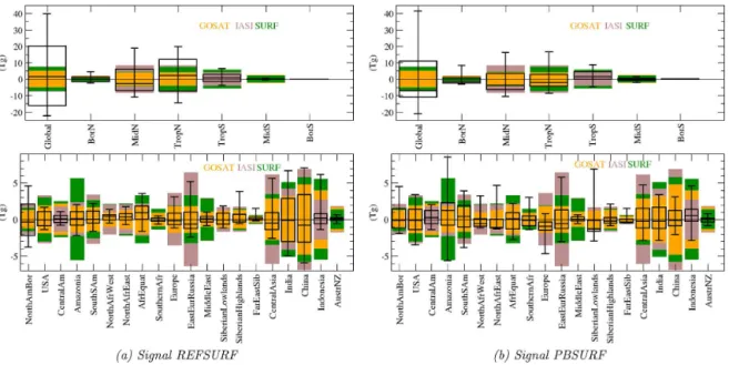
4.2 Impact of the signal on seasonal and yearly detection
Since the signal is obtained from one inversion only, it de-pends on a series of assumptions (error statistics, data selec-tion, etc.) and may have large uncertainties in various areas (e.g., far from the observing stations). Another signal defini-tion is therefore tested. We choose an inversion by Bousquet et al. (2011), (called PBSURF hereafter) instead of the REF-SURF inversion described above. Like REFREF-SURF, PBREF-SURF covers enough years of analysis to be representative of the variability of methane fluxes. The main differences between PBSURF and REFSURF are as follows:
Figure 8.Signal (Tg) for the four 3-year time windows at the pixel scale.
– Because of this, PBSURF solves for methane fluxes for large regions, whereas REFSURF works at the pixel scale.
– PBSURF retrieves monthly fluxes, whereas REFSURF retrieves fluxes at a weekly resolution.
– PBSURF solves for methane fluxes for several pro-cesses in each region, whereas REFSURF solves for net emissions.
– As a consequence of the three previous points, the B matrices of the two inversions are quite different. – PBSURF uses monthly means of the surface
observa-tions as constraints, whereas REFSURF uses hourly data.
– Because of this, the sets of surface stations used by PB-SURF and REFPB-SURF are different.
The large-region-scale inversion means that the spatial vari-ability of the prior is kept within each region and is only scaled (contrary to REFSURF, which is performed at the pixel scale, i.e., is able to vary only a few pixels to match the data). This difference in the methods may lead to very different spatial variability in each of the regions of interest (Fig. 4), a larger variability allowing a better detection rate with our criterion. Indeed, the large-region-scale inversion may lead to larger variability than pixel-based inversions in some regions (e.g., Pison et al. (2013)) because of the ho-mothetic scaling of the pixels composing each region in PB-SURF (correlations of 1 between pixels) as opposed to the
individual scaling of model pixels with soft constraints in REFSURF (spatial correlations less than 1).
We first focus on the seasonal (3-monthly) scale, which is the timescale at which the detection is the most favorable in the largest areas (Sect. 3.4) while being relevant for methane emissions at the regional scale defined here. The issue here is not whether the two inversions agree on the retrieved fluxes but whether the detection rates differ. Europe illustrates how the detection rates of two signals can differ; for GOSAT, sig-nal PBSURF is more than twice as often detected as REF-SURF and the signs of the detected anomalies are opposite (positive for REFSURF, mostly negative with PBSURF, Ta-bles 1 and A2; less positive anomalies are detected for a larger total number of detected anomalies).
Figure 9.Impact of spatial aggregation in Amazonia on noise (bars) and signal (box plots with median, 25 and 75 %) over 3-year time windows, from a unique pixel to larger rings around it. Detection is achieved when the signal is larger than the noise, i.e., for all the occurrences which lay outside the matching colored bar.
and NorthAfrEast, in which mainly positive anomalies are detected (IASI and SURF) or both positive and negative anomalies (GOSAT). The regional scale in the Southern Hemisphere confirms the better detection with signal PB-SURF (Amazonia, SouthSAm, SouthernAfr). In Amazonia, the (mainly positive) signals are detectable by GOSAT and IASI, but China (respectively India) is not any more (respec-tively poorly) detectable using PBSURF.
At the yearly scale (Table A3), the detection rates are shifted to the south (from TropN and MidN to TropS). De-tection rates higher than 50 % are found in Amazonia for GOSAT and IASI, and in Europe for GOSAT.
One important outcome of this sensitivity test to the sig-nal is that some regiosig-nal or hemispheric flux anomalies are detected but the localization of the detected signal varies de-pending on the inversion characteristics (including the ob-servations used). This is of course one important limitation in attributing the observed atmospheric changes to particular regions and to the underlying emission processes.
The impact of the signal on the detection of anomalies has also been tested by using a variational inversion at the
pixel scale assimilating both surface and IASI data. With this signal, the detection rates are higher in the tropics (partic-ularly in India and China) and in the Southern Hemisphere at midlatitudes (not shown). This suggests that the joint as-similation of surface and satellite data may lead to a better localization of the anomalies of the surface methane fluxes. Nevertheless, this requires that the consistency between the two types of data (surface and remote sensed) be improved (Locatelli et al., 2015; Monteil et al., 2013).
5 Conclusions
seasonal (3-month average) to long-term trend (3-year aver-age). At all scales, GOSAT generally shows the best results among the different systems, as could be expected from the density of the data and their sensitivity to surface emissions. At the regional scale, the results are more variable. In 8 regions out of 20, anomalies are detected by the three net-works; in 5 regions, no anomaly is detected by any of the three systems. The year-to-year changes are detected in 9 re-gions by GOSAT but with poor detection rates (lower than 40 %). Longer term trends (3-year averages) in African re-gions are detected with variable rates by the three systems. In some key regions for the methane cycle, anomalies are hardly detected, both in the case of dominant anthropogenic emissions (North America) or natural emissions (Amazo-nia, SiberianLowlands). A sensitivity test to the spatial scale through aggregation shows that dipole effects in the retrieved flux anomalies prevent anomalies in Amazonia (as defined in this study) to be detected. Flux anomalies in India and China, two areas with large and mixed (natural and anthropogenic) methane emissions, are generally poorly detected. A sensitiv-ity test with a second signal, also obtained from an inversion with surface constraints, shows that, overall, the detection at a yearly scale remains poor to fair (>50 % in Amazonia for the test signal). These tests point at the importance of prop-erly determining the spatial aggregation at which the inferred fluxes are used, with the issue that such an aggregation de-pends on the inversion system used. This suggests that the ability of the inversions to retrieve significant inter-annual variations in the methane fluxes is not evident and should be evaluated against uncertainties, which are not always com-puted and/or provided with the inversion products.
The use of another signal (which is from a different surface-based inversion) does not change the main conclu-sion that anomalies at the regional scale are not well detected but shows that the regions which are not seen may be differ-ent: some yearly changes in Amazonia can be detected but tropical Africa is much less detected with the second sig-nal. Therefore, the precise identification of flux anomalies in the tropics appears not to be robust with regard to changes in the inversion used for the signal. This is of course an is-sue when attributing the increase observed in atmospheric methane since 2006 to a particular region, as already noticed by Locatelli et al. (2015).
Our criterion is based on a 68 % confidence interval (1σ). At almost all regional space–time scales (except in NorthAmBor, AfrEquat at the longer timescales and a few cases in India, Indonesia, EastEurRussia and FarEastSib), the three observing systems would fail the test at 2σ (95 %), a more stringent criterion commonly used in other scien-tific communities. We also have neglected the impact of likely state-dependent systematic errors in current satellite retrievals and transport models that further reduce the inver-sion performance to an unknown extent.
Overall, our study may appear to be pessimistic about the skill of current inversions at the regional scale. However, at least two elements put this view into perspective.
First, we focused on the first decade of the 21st century, a time period with relatively flat methane signals. Neither a strong El Niño, nor a large volcanic eruption occurred, contrary to the previous decade (1990–1999). As an illus-tration, the methane atmospheric growth rate fluctuates from 2 to 16 ppb yr−1in the 1990s (standard deviation of yearly annual increase of ±4.5 ppb yr−1) as compared to −4 to +7 ppb yr−1(standard deviation of yearly annual increase of ±3.5 ppb yr−1) in the 2000s (Dlugokencky et al., 2011). This reduces methane flux anomalies and their detectability for a given noise. A time period with larger year-to-year changes in the methane cycle could lead to an improved detectability. Second, as mentioned in Sect. 2, we have been relatively conservative to estimate the noise, possibly leading to its overestimation, therefore also limiting the detectability of methane flux anomalies.
Our work has several implications for methane inversions. First, inversion results should never be presented without an extensive uncertainty analysis to distinguish between ro-bust and more hypothetical results. This may seem obvious but such an analysis is not always provided, or only partially, in inversion papers, mostly because of its computational cost. Second, to increase the detection robustness, the infor-mation amount from the satellite data and from the surface sites should be dramatically increased, as shown by the re-gional differences between the two surface-based inversions (e.g., Africa vs. tropical regions and China) and between the satellite-based inversions. Defining smaller regions, as tested here in Amazonia, may also improve the detection of anoma-lies in small key areas with intense methane emissions. An increase in the robustness of the attribution of flux anoma-lies to a particular region goes with the improvement of the consistency of error statistics prescribed for fluxes and obser-vations (Berchet et al., 2015).
Third, as the regions robustly inferred depend on the as-similated data sets, but also on the transport model and in-version setup, it seems important to push for regular com-parisons and syntheses of the various transport models and inversion systems, which is at present the only way to ap-proach the full range of uncertainty.
errors in passive satellite instruments (e.g., Buchwitz et al., 2016). Solar-based satellite instruments also provide limited data at high latitudes. The future space mission MERLIN, based on a differential active lidar measurement with a very small spot on the ground, should overcome these issues and provide data at all latitudes and all seasons (Kiemle et al., 2014). In this context, MERLIN seems to be a promising mission to improve some of the limitations raised in this pa-per.
6 Data availability
Appendix A: Appendix tables
Table A1.Yearly mean number of observations over the period used for the Monte Carlo noise computation (October 2009–September 2010) in the various regions for the three observing systems.
Region Area (×106km2) GOSAT IASI SURF
Global 510 32 348 240 084 1722
BorN 31 92 00 172
MidN 91 9060 00 556
TropN 126 14 934 121 756 602
TropS 128 6118 10 7148 156
MidS 95 2132 9078 140
BorS 37 00 00 96
NorthAmBor 14 194 00 00
USA 11 2516 2218 124
CentralAm 05 608 6328 24
Amazonia 07 802 3366 00
SouthSAm 10 1780 3068 24
NorthAfrWest 10 4986 4564 94
NorthAfrEast 07 3756 5148 00
AfrEquat 07 1394 3572 14
SouthernAfr 07 1488 3246 28
Europe 06 572 00 94
EastEurRussia 07 896 00 00
MiddleEast 06 2456 3748 26
SiberianLowlands 02 170 00 00
SiberianHighlands 05 126 00 00
FarEastSib 03 54 00 00
CentralAsia 12 3864 694 74
India 03 1180 4190 00
China 05 1164 4574 00
Indonesia 07 312 3324 26
Table A2.Detection of the signal consisting in the anomalies at the seasonal timescale (JFM, AMJ, JAS, OND). The signal is the difference between each quarter in the 2000–2011 period (i.e., 48 occurrences) and the 2004–2005 average from PBSURF. The noise is computed at the quarter timescale from each of the three observation systems, GOSAT, IASI and SURF. See Sects. 2.4 and 2.3 for details. In each cell of the table, we showX% (±T T) (±Y Y /±ZZ) whereX% is the percentage of quarterly anomalies detected, (±T T) is the difference with REFSURF (Table 1),±Y Yis the difference in the number of positive anomalies detected compared to REFSURF and±ZZis the difference in the total number of detected anomalies compared to REFSURF. Ave. mass indicates average emitted mass of CH4over 2004–2005.
Region GOSAT IASI SURF
Ave. mass (Tg) REFSURF/PBSURF
Global 517/499 87 % (−6) (−10/−3) 72 % (−19) (−9/−9) 72 % (−19) (−9/−9) BorN 18/17 75 % (+30) (+2/+14) 75 % (+36) (+5/+17) 77 % (+23) (0/+11) MidN 177/172 66 % (−11) (−2/−5) 35 % (−4) (0/−2) 62 % (−8) (0/−4) TropN 194/165 47 % (−40) (−10/−19) 27 % (−33) (−5/−16) 29 % (−37) (−6/−18) TropS 115/120 29 % (+21) (+9/+10) 31 % (+19) (+9/+9) 10 % (+10) (+5/+5)
MidS 12/25 ∅ ∅ 04 % (+4) (0/+2)
BorS 1/0 ∅ ∅ ∅
NorthAmBor 20/8 64 % (−15) (−2/−7) 43 % (−15) (+3/−7) 58 % (−17) (0/−8) USA 37/54 31 % (+31) (+8/+15) 06 % (+6) (+1/+3) 10 % (+10) (+3/+5)
CentralAm 17/13 ∅ 02 % (+2) (+1/+1) ∅
Amazonia 38/31 45 % (+31) (+19/+15) 35 % (+29) (+15/+14) 04 % (+4) (+2/+2) SouthSAm 30/45 45 % (+41) (+15/+20) 08 % (+8) (+3/+4) 20 % (+20) (+6/+10) NorthAfrWest 13/13 41 % (+31) (+7/+15) 16 % (+16) (+8/+8) 16 % (+16) (+8/+8) NorthAfrEast 11/12 39 % (+35) (+10/+17) 25 % (+25) (+12/+12) 25 % (+25) (+12/+12) AfrEquat 32/33 18 % (−4) (−10/−2) 10 % (−6) (−8/−3) 00 % (−2) (−1/−1) SouthernAfr 10/14 43 % (+43) (+7/+21) 14 % (+14) (+5/+7) 14 % (+14) (+5/+7) Europe 33/33 14 % (+8) (−3/+4) 04 % (+4) (0/+2) 12 % (+8) (−2/+4) EastEurRussia 30/27 33 % (0) (−2/0) ∅ 10 % (−6) (−3/−3)
MiddleEast 16/14 ∅ ∅ ∅
SiberianLowlands 8/14 89 % (+46) (+2/+22) 60 % (+58) (+11/+28) 85 % (+42) (+2/+20) SiberianHighlands 5/4 22 % (+14) (+7/+7) 12 % (+8) (+4/+4) 20 % (+16) (+8/+8) FarEastSib 1/2 52 % (+36) (+4/+17) 50 % (+42) (+8/+20) 50 % (+42) (+8/+20) CentralAsia 28/32 20 % (+14) (+5/+7) ∅ 08 % (+2) (+1/+1) India 50/45 10 % (−46) (−11/−22) 02 % (−33) (−5/−16) 00 % (−25) (0/−12) China 64/46 00 % (−14) (−3/−7) 00 % (−4) (0/−2) 00 % (−10) (−1/−5) Indonesia 36/33 06 % (0) (0/0) 12 % (+6) (+2/+3) 00 % (−4) (−2/−2)
Table A3.Detection of the signal consisting in the anomalies at the yearly timescale. The signal is the difference between each year in the 2000–2011 period (i.e., 12 occurrences) and the 2004–2005 average from PBSURF. The noise is computed at the yearly timescale from each of the three observation systems, GOSAT, IASI and SURF. See Sects. 2.4 and 2.3 for details. In each cell of the table, we showX% (±T T) (±Y Y /±ZZ) whereX% is the percentage of yearly anomalies detected, (±T T) is the difference with REFSURF (Table 2),±Y Y is the difference in the number of positive anomalies detected compared to REFSURF and±ZZis the difference in the total number of detected anomalies compared to REFSURF. Ave. mass indicates average emitted mass of CH4over 2004–2005.
Region
GOSAT IASI SURF
Ave. mass (Tg) REFSURF/PBSURF
Global 517/499 58 % (−17) (−1/−2) 66 % (−9) (0/−1) 4 %1 (−17) (−2/−2)
BorN 18/17 ∅ ∅ ∅
MidN 177/172 00 % (−8) (−1/−1) ∅ 00 % (−8) (−1/−1) TropN 194/165 00 % (−50) (−6/−6) ∅ 00 % (−25) (−3/−3) TropS 115/120 41 % (+25) (+3/+3) 41 % (+25) (+3/+3) 41 % (+25) (+3/+3)
MidS 12/25 ∅ ∅ ∅
BorS 1/0 ∅ ∅ ∅
NorthAmBor 20/8 25 % (+25) (+3/+3) ∅ ∅
USA 37/54 ∅ ∅ ∅
CentralAm 17/13 ∅ ∅ ∅
Amazonia 38/31 58 % (+50) (+7/+6) 58 % (+58) (+7/+7) 08 % (+8) (+1/+1) SouthSAm 30/45 33 % (+33) (+3/+4) 16 % (+16) (+2/+2) 16 % (+16) (+2/+2) NorthAfrWest 13/13 00 % (−33) (−4/−4) ∅ ∅
NorthAfrEast 11/12 00 % (−8) (−1/−1) ∅ ∅
AfrEquat 32/33 00 % (−33) (−4/−4) 00 % (−33) (−4/−4) 00 % (−25) (−3/−3)
SouthernAfr 10/14 16 % (+16) (+1/+2) ∅ ∅
Europe 33/33 50 % (+34) (−2/+4) 08 % (+8) (0/+1) 33 % (+33) (0/+4) EastEurRussia 30/27 16 % (+16) (+1/+2) ∅ ∅
MiddleEast 16/14 ∅ ∅ ∅
SiberianLowlands 8/+14 16 % (+16) (+1/+2) ∅ ∅ SiberianHighlands 5/4 00 % (−8) (−1/−1) ∅ ∅
FarEastSib 1/2 00 % (−8) (−1/−1) ∅ ∅
CentralAsia 28/32 00 % (−8) (0/−1) ∅ ∅
India 50/45 ∅ ∅ ∅
China 64/46 ∅ ∅ ∅
Indonesia 36/33 33 % (+17) (+2/+2) 33 % (+17) (+2/+2) ∅
Acknowledgements. The authors are very grateful to the many people involved in the surface and satellite measurement and in the archiving of these data. The authors particularly thank E. J. Dlugokencky (NOAA), S. A. Montzka (NOAA), C. Crevoisier (LMD), H. Boesch (University of Leicester), R. Parker (University of Leicester), P. B. Krummel (CSIRO), L. P. Steele (CSIRO), R. L. Langenfelds (CSIRO), S. Nichol (NIWA) and D. Worthy (EC). We acknowledge the contributors to the World Data Center for Greenhouse Gases for providing their data of methane and methyl-chloroform atmospheric mole fractions. The first author is funded by CNES and CEA. P. J. Rayner is in receipt of an Australian Professorial Fellowship (DP1096309). This work was performed using HPC resources from CCRT under the allocation 2014-t2014012201 made by GENCI (Grand Equipement National de Calcul Intensif) and a DSM allocation. We also thank the computing support team of the LSCE led by F. Marabelle.
Edited by: B. N. Duncan
Reviewed by: R. Kawa and one anonymous referee
References
Berchet, A., Pison, I., Chevallier, F., Bousquet, P., Bonne, J.-L., and Paris, J.-D.: Objectified quantification of uncertainties in Bayesian atmospheric inversions, Geosci. Model Dev., 8, 1525– 1546, doi:10.5194/gmd-8-1525-2015, 2015.
Bergamaschi, P., Frankenberg, C., Meirink, J., Krol, M., Dentener, F., Wagner, T., Platt, U., Kaplan, J., Körner, S., Heimann, M., Dlugokencky, E. J., and Goede, A.: Satellite chartography of at-mospheric methane from SCIAMACHY on board ENVISAT: 2. Evaluation based on inverse model simulations, J. Geophys. Res.-Atmos., 112, D02304, doi:10.1029/2006JD007268, 2007. Bergamaschi, P., Houweling, S., Segers, A., Krol, M.,
Franken-berg, C., Scheepmaker, R., Dlugokencky, E., Wofsy, S., Kort, E., Sweeney, C., Schuck, T., Brenninkmeijer, C., Chen, H., Beck, V., and Gerbig, C.: Atmospheric CH4in the first decade of the 21st century: Inverse modeling analysis using SCIAMACHY satellite retrievals and NOAA surface measurements, J. Geophys. Res.-Atmos., 118, 7350–7369, 2013.
Bousquet, P., Ciais, P., Miller, J. B., Dlugokencky, E. J., Hauglus-taine, D. A., Prigent, C., Van der Werf, G. R., Peylin, P., Brunke, E. G., Carouge, C., Langenfelds, R. L., Lathiere, J., Papa, F., Ramonet, M., Schmidt, M., Steele, L. P., Tyler, S. C., and White, J.: Contribution of anthropogenic and natural sources to atmospheric methane variability, Nature, 443, 439– 443, doi:10.1038/nature05132, 2006.
Bousquet, P., Ringeval, B., Pison, I., Dlugokencky, E. J., Brunke, E.-G., Carouge, C., Chevallier, F., Fortems-Cheiney, A., Franken-berg, C., Hauglustaine, D. A., Krummel, P. B., Langenfelds, R. L., Ramonet, M., Schmidt, M., Steele, L. P., Szopa, S., Yver, C., Viovy, N., and Ciais, P.: Source attribution of the changes in atmospheric methane for 2006–2008, Atmos. Chem. Phys., 11, 3689–3700, doi:10.5194/acp-11-3689-2011, 2011.
Buchwitz, M., Dils, B., Boesch, H., Crevoisier, C., and Detmers, R., Frankenberg, C., Hasekamp, O., Hewson, W., Laeng, A., Noel, S., Nothold, J., Parker, R., Reuter, M., and Schneis-ing, O.: Product Validation and Intercomparison Report (PVIR) for the Essential Climate Variable (ECV) Greenhouse Gases
(GHG), Tech. Rep. report version 4, ESA Climate Change Initia-tive (CCI), available at: http://www.esa-ghg-cci.org/?q=webfm_ send/300, last access: 10 February 2016.
Chevallier, F., Fisher, M., Peylin, P., Serrar, S., Bousquet, P., Breon, F., Chédin, A., and Ciais, P. F.: Inferring CO2 sources and sinks from satellite observations: Method and application to TOVS data, J. Geophys. Res., 110, D24309, doi:10.1029/2005JD006390, 2005.
Chevallier, F., Bréon, F.-M., and Rayner, P.: The contribution of the Orbiting Carbon Observatory to the estimation of CO2 sources and sinks: Theoretical study in a variational data assimilation framework, J. Geophys. Res., 112, D09307, doi:10.1029/2006JD007375, 2007.
Connor, B. J., Boesch, H., Toon, G., Sen, B., Miller, C., and Crisp, D.: Orbiting Carbon Observatory: Inverse method and prospec-tive error analysis, J. Geophys. Res.-Atmos., 113, D05305, doi:10.1029/2006JD008336, 2008.
Cressot, C., Chevallier, F., Bousquet, P., Crevoisier, C., Dlugo-kencky, E. J., Fortems-Cheiney, A., Frankenberg, C., Parker, R., Pison, I., Scheepmaker, R. A., Montzka, S. A., Krummel, P. B., Steele, L. P., and Langenfelds, R. L.: On the consistency between global and regional methane emissions inferred from SCIA-MACHY, TANSO-FTS, IASI and surface measurements, Atmos. Chem. Phys., 14, 577–592, doi:10.5194/acp-14-577-2014, 2014. Crevoisier, C., Nobileau, D., Fiore, A. M., Armante, R., Chédin, A., and Scott, N. A.: Tropospheric methane in the tropics – first year from IASI hyperspectral infrared observations, Atmos. Chem. Phys., 9, 6337–6350, doi:10.5194/acp-9-6337-2009, 2009. Desroziers, G., Berre, L., Chapnik, B., and Poli, P.: Diagnosis of
ob-servation, background and analysis-error statistics in observation space, Q. J. Roy. Meteor. Soc., 131, 3385–3396, 2005.
Dlugokencky, E., Steele, L., Lang, P., and Masarie, K.: The growth rate and distribution of atmospheric methane, J. Geophys. Res., 99, 17021–17043, doi:10.1029/94JD01245, 1994.
Dlugokencky, E., Bruhwiler, L., White, J., Emmons, L., Nov-elli, P., Montzka, S., Masarie, K., Crotwell, A., Miller, J., and Gatti, L.: Observational constraints on recent increases in the atmospheric CH4 burden, Geophys. Res. Lett., 36, L18803, doi:10.1029/2009GL039780, 2009.
Dlugokencky, E. J., Nisbet, E. G., Fisher, R., and Lowry, D.: Global atmospheric methane: budget, changes and dangers, Philos. T. R. Soc. Lond. A, 369, 2058–2072, doi:10.1098/rsta.2010.0341, 2011.
Francey, R., Steele, L., Langenfelds, R., and Pak, B.: High Preci-sion Long-Term Monitoring of Radiatively Active and Related Trace Gases at Surface Sites and from Aircraft in the Southern Hemisphere Atmosphere, J. Atmos. Sci., 56, 279–285, 1999. Gilbert, J.-C. and Lemaréchal, C.: Some numerical experiments
with variable-storage quasi-Newton algorithms, Math. Pro-gramm., 45, 407–435, 1989.
Hausmann, P., Sussmann, R., and Smale, D.: Contribution of oil and natural gas production to renewed increase in atmo-spheric methane (2007–2014): top–down estimate from ethane and methane column observations, Atmos. Chem. Phys., 16, 3227–3244, doi:10.5194/acp-16-3227-2016, 2016.
sensitivity to parametrized physics with emphasis on tropical convection, Clim. Dynam., 27, 787–813, 2006.
Houweling, S., Kaminski, T., Dentener, F., Lelieveld, J., and Heimann, M.: Inverse modeling of methane sources and sinks using the adjoint of a global transport model, J. Geophys. Res., 104, 26–137, 1999.
Kaminski, T., Rayner, P. J., Heimann, M., and Enting, I. G.: On ag-gregation errors in atmospheric transport inversions, J. Geophys. Res., 105, 4703–4715, 2001.
Kiemle, C., Kawa, S. R., Quatrevalet, M., and Browell, E. V.: Per-formance simulations for a spaceborne methane lidar mission, J. Geophys. Res.-Atmos., 119, 4365–4379, 2014.
Kirschke, S., Bousquet, P., Ciais, P., et al.: Three decades of global methane sources and sinks, Nat. Geosci., 6, 813–823, 2013. Locatelli, R., Bousquet, P., Hourdin, F., Saunois, M., Cozic, A.,
Couvreux, F., Grandpeix, J.-Y., Lefebvre, M.-P., Rio, C., Berga-maschi, P., Chambers, S. D., Karstens, U., Kazan, V., van der Laan, S., Meijer, H. A. J., Moncrieff, J., Ramonet, M., Scheeren, H. A., Schlosser, C., Schmidt, M., Vermeulen, A., and Williams, A. G.: Atmospheric transport and chemistry of trace gases in LMDz5B: evaluation and implications for inverse modelling, Geosci. Model Dev., 8, 129–150, doi:10.5194/gmd-8-129-2015, 2015.
Lowe, D., Brenninkmeijer, C., Tyler, S., and Dlugkencky, E.: Deter-mination of the Isotopic Composition of Atmospheric Methane and its Application in the Antarctic, J. Geophys. Res., 96, 15455– 15467, 1991.
Matthews, E., Fung, I., and Lerner, J.: Methane emission from rice cultivation: Geographic and seasonal distribution of cultivated ar-eas and emissions, Global Biogeochem. Cy., 5, 3–24, 1991. Monteil, G., Houweling, S., Butz, A., Guerlet, S.,
Schep-ers, D., Hasekamp, O., Frankenberg, C., Scheepmaker, R., Aben, I., and Röckmann, T.: Comparison of CH4 inver-sions based on 15 months of GOSAT and SCIAMACHY observations, J. Geophys. Res.-Atmos., 118, 11807–11823, doi:10.1002/2013JD019760, 2013.
Montzka, S., Krol, M., Dlugokencky, E., Hall, B., Jöckel, P., and Lelieveld, J.: Small interannual variability of global atmospheric hydroxyl, Science, 331, 67–69, doi:10.1126/science.1197640, 2011.
National Weather Service – Climate Prediction Cen-ter: Cold & Warm Episodes by Season, available at: http://www.cpc.ncep.noaa.gov/products/analysis_monitoring/ ensostuff/ensoyears.shtml, last access: 8 February 2016. Nisbet, E. G., Dlugokencky, E. J., Bousquet, P.: Methane on the
rise-again, Science, 343, 493–495, 2014.
Parker, R., Boesch, H., Cogan, A., Fraser, A., Feng, L., Palmer, P. I., Messerschmidt, J., Deutscher, N., Griffith, D. W., Notholt, J., Wennberg, P. O., and Wunch, D.: Methane observations from the Greenhouse Gases Observing SATellite: Comparison to ground-based TCCON data and model calculations, Geophys. Res. Lett., 38, L15807, doi:10.1029/2011GL047871, 2011.
Pison, I., Bousquet, P., Chevallier, F., Szopa, S., and Hauglus-taine, D.: Multi-species inversion of CH4, CO and H2emissions from surface measurements, Atmos. Chem. Phys., 9, 5281–5297, doi:10.5194/acp-9-5281-2009, 2009.
Pison, I., Ringeval, B., Bousquet, P., Prigent, C., and Papa, F.: Sta-ble atmospheric methane in the 2000s: key-role of emissions from natural wetlands, Atmos. Chem. Phys., 13, 11609–11623, doi:10.5194/acp-13-11609-2013, 2013.
Rigby, M., Prinn, R., Fraser, P., Simmonds, P., Langenfelds, R., Huang, J., Cunnold, D., Steele, L., Krummel, P., Weiss, R., O’Doherty, S., Salameh, P., Wang, H., Harth, C., Mülhe, J., and Porter, L.: Renewed growth of atmospheric methane, Geophys. Res. Lett., 35, L22805, doi:10.1029/2008GL036037, 2008. Schaefer, H., Fletcher, S. E. M., Veidt, C., Lassey, K. R.,
Brails-ford, G. W., Bromley, T. M., Dlugokencky, E. J., Michel, S. E., Miller, J. B., Levin, I., Lowe, D. C., Martin, R. J., Vaughn, B. H., and White, J. W. C.: A 21st-century shift from fossil-fuel to bio-genic methane emissions indicated by13CH4, Science, 352, 80– 84, doi:10.1126/science.aad2705, 2016.