www.atmos-chem-phys.net/16/6863/2016/ doi:10.5194/acp-16-6863-2016
© Author(s) 2016. CC Attribution 3.0 License.
Cluster analysis of European surface ozone observations for
evaluation of MACC reanalysis data
Olga Lyapina1, Martin G. Schultz1, and Andreas Hense2
1Forschungszentrum Jülich, Institute for Energy and Climate Research: Troposphere (IEK-8), Jülich, 52425, Germany 2Meteorological Institute, Bonn University, Bonn, 53121, Germany
Correspondence to:Martin G. Schultz ([email protected])
Received: 30 November 2015 – Published in Atmos. Chem. Phys. Discuss.: 8 February 2016 Revised: 6 April 2016 – Accepted: 14 April 2016 – Published: 6 June 2016
Abstract.The high density of European surface ozone mon-itoring sites provides unique opportunities for the inves-tigation of regional ozone representativeness and for the evaluation of chemistry climate models. The regional rep-resentativeness of European ozone measurements is exam-ined through a cluster analysis (CA) of 4 years of 3-hourly ozone data from 1492 European surface monitoring stations in the Airbase database; the time resolution corresponds to the output frequency of the model that is compared to the data in this study. K-means clustering is implemented for seasonal–diurnal variations (i) in absolute mixing ratio units and (ii) normalized by the overall mean ozone mix-ing ratio at each site. Statistical tests suggest that each CA can distinguish between four and five different ozone pol-lution regimes. The individual clusters reveal differences in seasonal–diurnal cycles, showing typical patterns of the ozone behavior for more polluted stations or more rural back-ground. The robustness of the clustering was tested with a series of k-means runs decreasing randomly the size of the initial data set or lengths of the time series. Except for the Po Valley, the clustering does not provide a regional differentia-tion, as the member stations within each cluster are generally distributed all over Europe. The typical seasonal, diurnal, and weekly cycles of each cluster are compared to the output of the multi-year global reanalysis produced within the Mon-itoring of Atmospheric Composition and Climate (MACC) project. While the MACC reanalysis generally captures the shape of the diurnal cycles and the diurnal amplitudes, it is not able to reproduce the seasonal cycles very well and it exhibits a high bias up to 12 nmol mol−1. The bias de-creases from more polluted clusters to cleaner ones. Also, the seasonal and weekly cycles and frequency distributions
of ozone mixing ratios are better described for clusters with relatively clean signatures. Due to relative sparsity of CO and NOxmeasurements these were not included in the CA.
How-ever, simulated CO and NOx mixing ratios are consistent
with the general classification into more polluted and more background sites. Mean CO mixing ratios are within 140– 145 nmol mol−1(CL1–CL3) and 130–135 nmol mol−1(CL4 and CL5), and NOxmixing ratios are within 4–6 nmol mol−1
and 2–3 nmol mol−1, respectively. These results confirm that relatively coarse-scale global models are more suitable for simulation of regional background concentrations, which are less variable in space and time. We conclude that CA of sur-face ozone observations provides a powerful and robust way to stratify sets of stations, being thus more suitable for model evaluation.
1 Introduction
Numerical models of atmospheric transport and chemistry (CTMs) have become indispensable tools for the interpre-tation of measurement data, the analysis of sensitivities to-wards, for example, emission changes, and the evaluation of potential future air quality changes in the context of climate change.
Since 2005, a major European effort is under way to establish an operational system for monitoring and pre-dicting global and European air quality with the help of data assimilation and numerical models (Hollingsworth et al., 2008). This Copernicus Atmosphere Monitoring Service (http://www.copernicus-atmosphere.eu/) has been developed in a series of projects funded by the European Commission under the acronym of Monitoring Atmospheric Composition and Climate (MACC). One of the products from MACC is a global reanalysis of atmospheric chemical composition cov-ering the period 2003–2012 (Inness et al., 2013).
The quality of all model-based estimates of atmospheric composition and its changes has to be assessed by in-depth model evaluations against observations. Currently model evaluation is often performed either on individual observa-tions or on the average of the set of measurements, selected from specific geographical regions. This is done for evalu-ation of global (Stevenson et al., 2006; Fiore et al., 2009; Lamarque et al., 2012; Katragkou et al., 2015) as well as re-gional (van Loon et al., 2007; Coman et al., 2012; Solazzo et al., 2012; Mailler et al., 2013) models or their ensemble. This approach is problematic because there is no guarantee that the regional average of selected stations gives a represen-tative picture of the ozone distribution in that region. Further-more there is large variability of ozone regimes even on small spacial scales, and models will not be able to capture this variability unless they are run on very fine resolution. There-fore, rather than aggregate data geographically we propose evaluating models based on groups of stations which share common characteristics with respect to their ozone seasonal and diurnal cycles.
In the Airbase database (http://acm.eionet.europa.eu/ databases/airbase/) more than 4000 stations from 39 Euro-pean countries are classified based on the evaluation of the population distribution and emission sources in the proximity of the station. This scheme was defined in the Council Deci-sion 97/101/EC (EC DeciDeci-sion, 1997), which was revised and amended by Commission Decision 2001/752/EC (EC sion, 2001) and finally modified by 2011/850/EU (EC Deci-sion, 2011) and described in Mol et al. (2008).
Analysis of the population distribution distinguishes the station type between urban, suburban, and rural, while the as-sessment of emission sources in the surrounding area divides sites into traffic, industrial, or background. Such categoriza-tion has the disadvantage of being based on subjective assess-ments by the different station maintainers or regional agen-cies. Moreover the station information may become outdated, for example due to newly built industries, residential areas, roads, or changes to forest areas. Such changes would
trans-form stations from “background” to “urban”, which would impede objective ozone analysis. Thus, a static category la-bel as given in Airbase may not provide an objective and reproducible classification for use in further statistical analy-ses. Instead, we suggest applying cluster analysis (CA) to the measurement data as a data-driven classification. The main goal of this study is to identify typical European air qual-ity ozone regimes, determine their indicative patterns with respect to the temporal behavior of ozone mixing ratios, to assess how well the classification works, and apply the cat-egorization to the evaluation of a global chemistry transport model. Analysis of group separation was presented in Lyap-ina (2015) and will not be discussed here.
The output from the MACC reanalysis was sampled at all station locations, and the results were grouped into the same clusters as the measurement data. Through comparison of the mean seasonal, weekly, and diurnal cycles and anal-ysis of the variability of clusters, we can identify how well the MACC reanalysis can reproduce the ozone mixing ratios and seasonal–diurnal features of each regime and, as a con-sequence, which regime is most consistent with the model results and thus representative for the scale of the model.
The paper is structured as follows: Sect. 2 describes the process of data filtering from the full Airbase database. The extraction conditions for the MACC model data are given as well as further steps of the preparation of both data sets. Sec-tion 3 provides details about the appliedk-means algorithm and Earth mover’s distance (EMD) method. In Sect. 4 the results of the two CAs are presented and compared to the MACC model data. Section 5 discusses the robustness of the cluster analyses and their application for the evaluation of models. Section 6 contains the conclusions.
2 Data 2.1 Airbase
convert measurements at actual temperature and pressure to these standard conditions.
Several data sets in Airbase contain incomplete data and some ozone records appear unreliable. Therefore a four-step filtering procedure was applied to each data set in order to identify suitable time series and to remove individual out-liers which could corrupt the time series statistics. First, all data less than 0 were eliminated, because they represent non-physical values. Next, data above either 2.83 times the value of the 95th percentile of the data or twice the value of the 99th percentile were eliminated. For a Gaussian distributed random variable both values should be approximately iden-tical. Even though the ozone probability density functions are generally not Gaussian (see Fig. 9), this test can be used to define a reasonable upper limit value, because deviations from the normal distribution are mainly at the lowest per-centile range of data. In a third step, those data points were removed which show erratic behavior near a missing value. The rationale behind this test is that a visual inspection of measurement time series sometimes indicates that data re-porting stopped too late or resumed too early after a calibra-tion procedure, an instrument maintenance, or malfunccalibra-tion. On each side of the missing value, the five nearest measure-ments are tested if they lie in the range of the surrounding values or exhibit abnormal variability. Finally, another outlier test (multi-step low-pass filter) was performed using the 240 data points moving average in the first pass, which removed data points exceeding 8 times the standard deviation within the moving sample. In the next two passes with a varying width between 10 and 72 points, thresholds of 8 and 6 stan-dard deviations are applied.
The data filtering was tested extensively on many different ozone time series and found to reliably detect obvious errors while removing only very few valid data points. In order to retain a time series in the analysis it had to fulfill the fol-lowing data capture criterion: in every year, at least 9 out of 12 months had to contain at least two-thirds of the theoretical maximum hourly values. After application of this criterion, the original Airbase data set of more than 4000 stations was reduced to 1525 stations (see Tables S1 and S2 in the Sup-plement). Their time series were then visually inspected for sudden changes in the baseline (this phenomenon is not cap-tured by the automated data quality filter; see also Solberg et al., 2009). We adopted a conservative approach and flagged only those stations, where baseline shifts of 5 nmol mol−1or greater occurred. The 33 stations which were filtered out at this step are presented in Table S2. Finally 1492 sites were used in the CA and model evaluation (Table S1).
As input for the CA multi-annual monthly mean diurnal variations averaged over the 4-year period 2007–2010 of the individual ozone time series were used. Seasonal–diurnal ozone variations appear as typical cycles and represent the concentrations resulting from many factors influencing the particular stations. We used 3 h resolution rather than the original hourly resolution in order to match the frequency
of the MACC model output (see Sect. 2.2). Thus each station is represented by a vector of dimension 96 (12 months times 8 time steps per day). The time averaged data at all stations were arranged as a data matrix of dimension 1492 by 96.
Two different input matrices for the CA were constructed leading to two different types of CA runs (first CA and sec-ond CA from here on). First, seasonal–diurnal ozone varia-tions in absolute values are used as a set of properties. Sec-ond, we used normalized seasonal–diurnal ozone variations in order to avoid the influence of actual ozone concentrations on the results. Each normalized variation had 0 mean and unit standard deviation. This second CA produces different clus-ters than the first step but allocates stations to clusclus-ters based on seasonal and diurnal variations themselves, regardless of absolute concentrations. Since the data generally exhibit no trend during the 2007–2010 period and interannual variabil-ity is much smaller than the diurnal or seasonal variabilvariabil-ity, we did not detrend the data prior to the CA.
2.2 MACC
The model data were taken from the MACC reanalysis (In-ness et al., 2013). The reanalysis invoked data assimilation of meteorological variables, trace gas columns of O3, CO, NO, and NO2, as well as ozone profile information from various satellite instruments. The model system was the European Centre for Medium Range Weather Forecasts (ECMWF) Integrated Forecasting System, which was coupled to the Model for Ozone and Related Tracers (MOZART) (Flem-ming et al., 2009; Stein et al., 2012). The model grid resolu-tion was about 80 by 80 km2, with 60 hybrid sigma-pressure levels covering the atmosphere from the surface to about 60 km altitude. Output was stored every 3 h. We extracted gridded time series for the years 2007–2010. The model data at the 1492 Airbase stations used in the cluster analysis were obtained by a horizontal as well as vertical bi-linear interpo-lation to the locations and heights of the 1492 Airbase sta-tions from the eight nearest neighboring grid points. Similar to O3, CO, and NOx were also extracted and provided as
mole fractions.
3 Method
3.1 Cluster analysis
CA is a data-driven technique for classifying objects into groups whereby each object is described through a set of in-put parameters (properties or variables) which are used as criteria for grouping. Clusters are formed such that the in-tra cluster similarity between objects inside a cluster and the inter cluster dissimilarity between objects of different clusters are jointly maximized. Initially the concept of CA was suggested by Tryon (1939). Since then it has found applications in statistical processing of large data sets in biology, medicine, computer science, meteorology, and at-mospheric sciences (Zhang et al., 2007; Lee and Feldstein, 2013; Camargo et al., 2007; Christiansen, 2007; Beaver and Palazoglu, 2006; Dorling and Davies, 1995; Marzban and Sandgathe, 2006), as well as in other fields.
Several cluster algorithms have been developed and dif-ferent choices can be made for the computation of distances between objects or groups of objects. The most commonly used types of clustering are hierarchical and partitional (aka centroid-based clustering ork-means clustering). Hierarchi-cal clustering progressively splits the data set into more and finer clusters, whereas partitional clustering groups the data into a pre-determined number of clusters. Clusters are non-overlapping groups, such that at the end of the computation each object will belong to exactly one cluster. In the present study we applied partitional clustering, because it allows for estimating the robustness of results and is less sensitive to outlier values than hierarchical clustering.K-means uses the Euclidean metricEdistfor the calculation of distances:
Edist(AB)= 2 v u u t
M X
m=1
(xmA−xmB)2, (1)
wherexA andxBare two objects of the data set, each with Mproperties (i.e., variables); A and B are two different sta-tions. In our case an object is a station time series of monthly averaged diurnal variations of 3-hourly ozone concentrations such that the Euclidean distance is evaluated from M=96 dimensions and is identical to the root mean square error between the two objects. The first CA uses absolute mix-ing ratio values, while in the second CA the mixmix-ing ratios at each station are normalized by the mean so that each ob-ject had zero ozone mean and unit standard deviation. Thek -means algorithm minimizes the average Euclidean distances between individual objects and the given number of cluster centroids. A centroidcis an artificial object that represents its cluster and is the arithmetic mean of all properties of clus-ter members:
ci=
1 ni
ni X
j=1
xij, (2)
Figure 1.Averaged SSD (“elbow” plot) of 50·100 independentk -means runs with varying number of clusterskfrom 1 to 100, based on the first set of properties.
whereniis the number of objects inith cluster,ciis the
cen-troid of theith cluster, andxijis thejth object of theith
clus-ter. Minimization is achieved iteratively in an analysis cycle of three steps. At the initial step of eachk-means run,k cen-troids are defined randomly from the data array. The second step assigns each object to the closest centroid by sorting in ascending order the distancesEdist(Aci). Through this an
ini-tial seed of clusters is formed. In the third step, each centroid cis recalculated as the mean of the current cluster members. Steps 2 and 3 are then repeated until the centroid coordinates no longer change. The goodness of the clustering can be as-sessed with the sum of squared distances (SSD) between all objects and their corresponding centroids:
SSD=
k X
i=1 Xnk
j=1Edist(ci, xij) 2,
(3)
wherekis the number of clusters, andnkis the number of
Figure 2.Averaged SSD (“elbow” plot) of 50·100 independentk -means runs with varying number of clusterskfrom 1 to 100, based on the second set of properties.
The elbow plots not only give the appropriate number of clusters to runk-means, but they also provide a preliminary answer on the question of stability of the CA run for the cho-sen k. For the presentation of results in Sects. 4 and 5 we picked thek-means run with the lowest SSD out of the 100 independent realizations shown in Figs. 20 and 21, respec-tively, for each kind of CA. Further details on the stability (i.e., reproducibility) ofk-means runs are given in Sect. 5. 3.2 Earth mover’s distance
In order to quantitatively evaluate the model’s ability to re-produce the observed frequency distributions in each cluster, we calculated the EMD. Initially the EMD was suggested by Rubner et al. (1998). EMD provides an objective distance measure between two frequency distributions or estimates of probability density functions. It is a true distance measure in the sense that it is positive semi-definite and symmetric and fulfills the triangle inequality. Additionally it has the property of being (asymptotically) proper, meaning that the smallest distance is only achieved when the two probability densities are identical. The formula for EMD according to Rabin et al. (2008) is
D(f||g)= 1
nb nb X
i=1
|FX(xi)−GX(xi)|, (4)
wherenb is the number of bins, andFX(xi) andGX(xi) are two cumulative distribution functions of f and g, which themselves are the two corresponding estimated probability densities obtained from the normalization of the respective frequency distribution histograms over thenbbins.
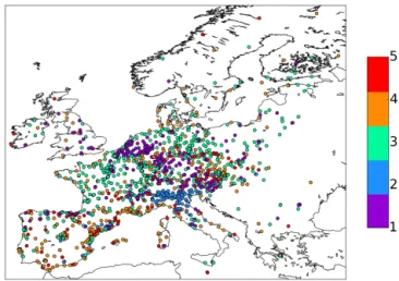
Figure 3.Map of 1492 Airbase stations clustered in five groups; first CA.
4 Results and discussion
4.1 Geographical distribution and cluster allocation of stations
4.1.1 First CA
The spatial distribution of the 1492 Airbase stations and the respective cluster number of their classification obtained af-ter the first CA are shown in Fig. 3. Evidently, the five clus-ters do not simply represent different regions in Europe, al-though the members of cluster 1 (CL1) and cluster 2 (CL2) are concentrated in the Benelux and Ruhr regions and in the Po Valley region, respectively. CL1 extends from Slovenia to Great Britain through the Netherlands but also includes sta-tions in France, Italy, Spain, and Eastern Europe. Besides the northern Italian stations CL2 also contains a few stations in the Alpine region, in the northwestern Balkans and in Spain. The third cluster (CL3) is much larger in its spatial extension and contains stations from almost all over Europe, including Scandinavia. The fourth cluster (CL4) spreads all over Eu-rope with increased density along the Mediterranean coast and in the mountainous areas to the north and east of the Alps, the Bohemian Massif, and the Carpathian Mountains. Finally, the smallest cluster (CL5) largely overlaps with the mountainous regions of the Alps, the Pyrenees, Spain, and the Carpathians.
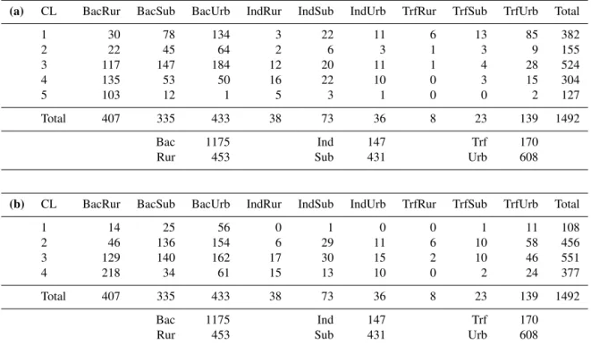
“back-Table 1. (a)Contingency table, showing the distribution of stations in clusters (rows) vs. Airbase classification groups (columns); first CA. Abbreviations: Bac – background, Ind – industrial, Trf – traffic, Rur – rural, Sub – suburban, Urb – urban.(b)Same as(a)but for the second CA.
(a) CL BacRur BacSub BacUrb IndRur IndSub IndUrb TrfRur TrfSub TrfUrb Total
1 30 78 134 3 22 11 6 13 85 382
2 22 45 64 2 6 3 1 3 9 155
3 117 147 184 12 20 11 1 4 28 524
4 135 53 50 16 22 10 0 3 15 304
5 103 12 1 5 3 1 0 0 2 127
Total 407 335 433 38 73 36 8 23 139 1492
Bac 1175 Ind 147 Trf 170
Rur 453 Sub 431 Urb 608
(b) CL BacRur BacSub BacUrb IndRur IndSub IndUrb TrfRur TrfSub TrfUrb Total
1 14 25 56 0 1 0 0 1 11 108
2 46 136 154 6 29 11 6 10 58 456
3 129 140 162 17 30 15 2 10 46 551
4 218 34 61 15 13 10 0 2 24 377
Total 407 335 433 38 73 36 8 23 139 1492
Bac 1175 Ind 147 Trf 170
Rur 453 Sub 431 Urb 608
Table 2.Cluster statistics and description based on the Airbase classification, geographical location, and altitude range of clusters; first CA.
CL Cluster description Number of stations Mean altitude, m (25. . . 75th percentiles)
1 urban traffic 382 177 (35. . . 250)
2 urban/suburban, Po Valley 155 243 (72. . . 381)
3 urban/suburban 524 203 (50. . . 287)
4 rural/industrial/remote, middle-elevated 304 288 (45. . . 503)
5 rural background, elevated 127 819 (370. . . 1137)
ground” according to the station type. Each row in Table 1 corresponds to one of the Airbase clusters and shows the number of stations related to each of nine Airbase classifi-cation pairs. Most of the stations that we retained in our data filtering procedure (Sect. 2) are background stations, which could indicate that there are no local pollution sources in their vicinity. Measured concentrations should ideally be repre-sentative for a larger area (and hence suitable for the eval-uation of numerical models), except when local effects from orography, land use, or land–sea contrast confound the anal-ysis. There is a relatively even split between rural, suburban, and urban background stations. Industrial and traffic stations constitute about 10–15 % each and are concentrated in the suburban and urban environments, respectively.
4.1.2 Second CA
Table 3 presents the same information as Table 2 but for the second CA. There is some overlap between the cluster
def-initions of the first and second CA. The first cluster of the second CA corresponds to the second cluster of the first CA, with the exception that it does not contain stations from the Alpine region (Fig. 4). The second cluster is much larger and spreads over the Benelux and Ruhr regions in the center of Europe, partly covering France, Switzerland, and Eastern Eu-rope and thus partially overlapping with the first cluster from the first CA.
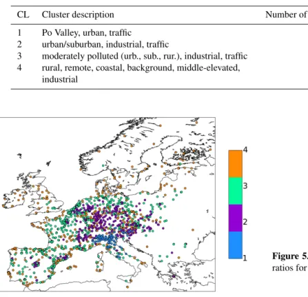
Table 3.Cluster statistics and description based on the Airbase classification, geographical location, and altitude range of clusters; second CA.
CL Cluster description Number of stations Mean altitude, m (25. . . 75th percentiles)
1 Po Valley, urban, traffic 108 200 (45. . . 293)
2 urban/suburban, industrial, traffic 456 250 (90. . . 360)
3 moderately polluted (urb., sub., rur.), industrial, traffic 551 190 (35. . . 273) 4 rural, remote, coastal, background, middle-elevated,
industrial
377 433 (35. . . 735)
Figure 4.Map of 1492 Airbase stations clustered in four groups; second CA.
with Airbase metadata (Table 1) and the geographical repre-sentation lead to the conclusion that the clusters from differ-ent CAs have some common features. For example, the first Po Valley cluster of the second CA, which is mostly concen-trated in the north of Italy, is the same as the second cluster of the first CA. The second cluster of the second CA has the majority of stations, which were assigned to the first cluster in the first CA, and moreover also captures stations of the second and third clusters of the first CA. However, it appears as more elevated agglomeration. The third cluster shares 326 stations out of more than 500 with the third cluster of the first CA, resembling it also geographically and in altitude. It is the largest cluster in both CAs. The fourth cluster of the second CA contains both high- and low-altitude stations. It includes the entire fifth cluster and has some stations from the fourth and third clusters of the first CA. Therefore, on average the fourth cluster of the second CA with the mean altitude of 433 m is semi-elevated.
Figure 5.Percentiles (5–25–50–75–95) of 3-hourly ozone mixing ratios for 1492 stations; Airbase vs. MACC.
4.2 Comparison of Airbase clusters with MACC model results
4.2.1 Ozone means and consistency with ozone precursor concentrations
Figure 5 presents a comparison of the 5–25–50–75–95th per-centiles distributions from the 3-hourly Airbase and MACC initial data sets for the period 2007–2010 (i.e., length of each data set= 1492 stations·4 years·365 days·8 values per day). The mean and median volume mixing ratios averaged over the entire set of 1492 stations are 25 and 24 nmol mol−1 for Airbase and 34 and 33 nmol mol−1 for MACC, respec-tively. Thus the 50th percentile and the mean of the model data both show a positive bias of 9 nmol mol−1.
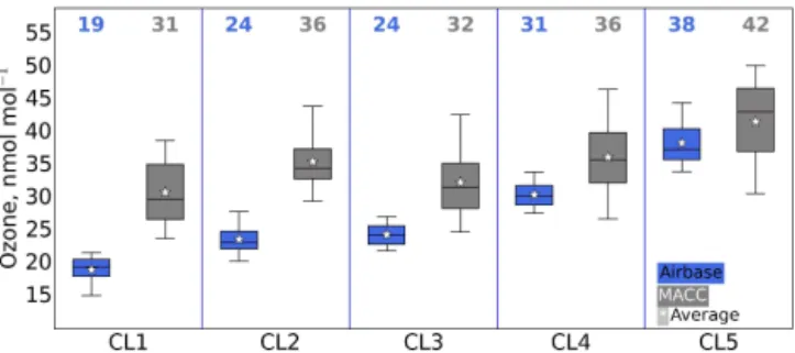
A more detailed pattern emerges when analyzing the sta-tion mean values using box-and-whisker plots separately for the five individual clusters of the first CA (Fig. 6). With the exceptions of CL2 and CL3, which show quite similar distri-butions, the distributions of the observed (Airbase) values are rather distinct for each cluster and increase from CL1 to CL5. In comparison, the MACC distributions are generally broader and exhibit a high bias of 5–12 nmol mol−1, except for CL5. MACC distributions also show increasing values from CL3 to CL5 but only little difference among CL1 to 3. Obviously, the model does not capture the differences among the some-what more polluted sites very well. This is consistent with the distributions of simulated CO and NOx concentrations
meaning-Figure 6.Percentiles (5–25–50–75–95) of ozone means in clusters; Airbase vs. MACC, first CA. Upper values indicate the mean of each cluster.
Figure 7. Percentiles (5–25–50–75–95) of modeled CO (a)and NOx(b)means in clusters; first CA.
ful comparison) shown in Fig. 7. While the MACC model re-sults show a clear separation between clusters 1–3 on the one hand and clusters 4–5 on the other hand, they do not distin-guish among CL1, 2, and 3. These results are not surprising given that ozone concentrations in CL1–CL3 are more likely influenced by local, small-scale pollution sources, which the model cannot simulate correctly with its grid point distance of approximately 80 km. It is, however, reassuring to see that the simulated mean values of ozone precursors are larger in those clusters that have been labeled more polluted according to the Airbase characterization tags.
Figure 8 shows the distributions of mean ozone mixing ratios in the clusters of the second CA. The MACC distribu-tions of mean values are again broader than the observadistribu-tions and the model overestimates all clusters with the highest bias of 14 nmol mol−1 for CL1 and the lowest 4 nmol mol−1for CL4. The distribution of observed ozone means of CL4 is
Figure 8.Percentiles (5–25–50–75–95) of ozone means in clusters; Airbase vs. MACC, second CA. Upper values indicate the mean of each cluster.
broader than it is in the first CA. This can be explained by the mix of stations of various altitudes. For other clusters, the distributions are relatively narrow but still nearly twice as broad as those of the first CA, except for CL1 (Fig. 6). MACC model distributions of CO and NOx concentrations
for the clusters of the second CA (not shown) are reflecting higher pollution levels in the first two clusters and moder-ate pollution conditions for CL3. CL4 is relatively clean and shows the lowest CO and NOxconcentrations.
4.2.2 Frequency distributions of ozone in clusters
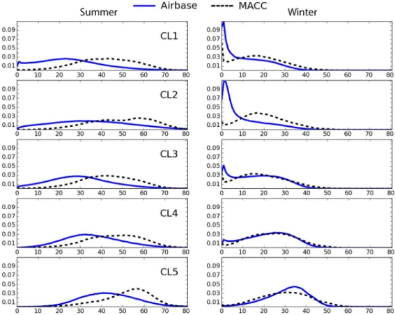
The comparison of ozone concentrations among the clus-ters and between the observations and the simulations was based upon quantiles characterizing the cumulative probabil-ity distribution. Another way is to estimate probabilprobabil-ity den-sity functions or normalized frequency distributions com-puted by binning all available 3-hourly observations from both the Airbase and MACC data. Those frequency distri-butions are presented in Fig. 9 for each cluster of the first CA and distinguished between summer and winter.
In the Airbase wintertime data the three clusters with more urban characteristics (CL1, CL2, and CL3) contain a signif-icant number of values with very low concentrations, which are primarily caused by ozone titration in the presence of large amounts of NOx from traffic and industries. Peak
fre-quencies are decreasing from CL1 to CL4, though the last shows only a few incidents of “zero” ozone. For clusters CL1, CL3 and CL4 the MACC model is able to capture some of this titration, but not for CL2 (Po Valley). No ozone titra-tion occurs in CL5, either in the observatitra-tional data or in the model results.
Figure 9.Normalized frequency distributions of 3-hourly ozone values in clusters (2007–2010), in summer (left) and winter (right); Airbase vs. MACC, first CA.
Figure 10.Normalized frequency distributions of 3-hourly ozone values in clusters (2007–2010); Airbase vs. MACC, second CA.
In order to quantitatively evaluate the model’s ability to reproduce the observed frequency distributions in each clus-ter, we calculated the EMD (described in Sect. 3) (Table 4). As expected from Fig. 9, the largest EMD is found for CL1 and CL2 in summer, while the model shows greater skill in capturing the frequency distributions of CL4 and CL5 and to a lesser extent also CL3 (Table 4). This is again consistent with the previous characterizations of CL3 as a background, moderately polluted station and of CL4 and CL5 as (mostly
Table 4.EMD values for each cluster between Airbase and MACC data (2007–2010); first CA.
CL Summer Winter All
1 0.181 0.068 0.126
2 0.146 0.112 0.134
3 0.139 0.028 0.083
4 0.110 0.021 0.064
5 0.092 0.025 0.041
Table 5.EMD values for each cluster between Airbase and MACC data; second CA.
CL EMD (obs–mod)
1 0.15
2 0.106
3 0.091
4 0.051
where MACC fails to predict the very low concentrations (Table 4, Fig. 9).
Frequency distributions of the 3-hourly surface ozone val-ues of Airbase and MACC for each cluster of the second CA are presented in Fig. 10. As anticipated from the pre-vious discussion, clusters with urban signatures CL1 and CL2 are expected to show a peak at low ozone concen-trations, related to their higher pollution level. Indeed, the peaks of Airbase probabilities of zero ozone concentrations are pronounced for both clusters in comparison to the mod-erately polluted CL3, for example, where zero ozone occurs only half as often and the ozone maximum appears in the range 25–30 nmol mol−1. The shape of the relatively clean CL4 curve resembles a Gaussian distribution with maximum probability at ≈35 nmol mol−1. EMD calculated for com-parison of observations to modeled frequency distributions (Table 5) show the strongest disagreement for CL1, followed by CL2 and CL3 with quite similar values, and finally is the smallest EMD value for CL4.
4.3 Analysis of seasonal, diurnal, and weekly variations 4.3.1 First CA
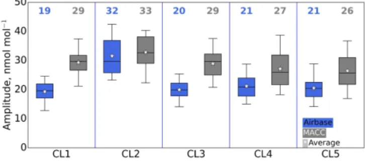
The mean seasonal amplitudes are defined as the differ-ence between the highest and lowest 4-year average monthly mean ozone concentrations (Fig. 11). The amplitudes esti-mated from the Airbase stations within the clusters of the first CA are generally between 18 and 24 nmol mol−1(25th to 75th percentiles), with the exception of CL2 (Po Val-ley stations), where seasonal amplitudes range from about 26 to 37 nmol mol−1(25th to 75th percentiles). The MACC model data show a similar pattern among the clusters. How-ever, the seasonal amplitude is often overestimated by 5–
Figure 11.Percentiles (5–25–50–75–95) of ozone seasonal ampli-tudes in clusters; Airbase vs. MACC, first CA. Upper values indi-cate the mean seasonal amplitude of each cluster.
10 nmol mol−1 due to the overestimation of summertime ozone. The seasonal amplitude of CL2 stations is captured relatively well, although the mean values in CL2 exhibited the second highest bias (12 nmol mol−1, Fig. 6).
The seasonal cycles of the first CA cluster centroids are displayed in Fig. 12. In the observations CL1 and CL3 run almost parallel and show a broad maximum extending from April to July for CL1 and a slight maximum in April for CL3. More prominent spring maxima are evident in CL4 and CL5, but CL5 also exhibits a second small peak in July. The only cluster with a single pronounced maximum in summer (July) is CL2. The spring maximum is typical for seasonal cycles of western European sites and considered a northern hemi-spheric phenomenon (Monks, 2000). Indeed, a substantial subset of stations in CL3, CL4, and CL5 are situated along the western edge of the continent (see map, Fig. 3). The de-cline of ozone mixing ratios from spring until autumn in CL3 and CL4 suggests that summer photochemical ozone forma-tion plays only a minor role at these sites. In contrast, the double peak of CL5 suggests a superposition of the “natural” spring maximum with the “anthropogenic” summertime pho-tochemical ozone production. The stations in CL5 are more elevated and therefore can be influenced by ozone from the stratosphere–troposphere exchange, which is considered as a possible reason for the ozone spring maximum on high mountains (Elbern et al., 1997; Harris et al., 1998; Stohl et al., 2000; Monks, 2000; Zanis et al, 2003).
In contrast to the seasonal cycles of the Airbase cluster centroids, the cluster mean seasonal cycles of the MACC data all show a summer maximum of similar shape with peak in June. This suggests that either the summertime chemical ozone formation is exaggerated in the model or the largely transport-driven springtime maximum is underestimated. A potential influence from inconsistencies in the data assimi-lation (see Inness et al., 2013) is unlikely, but it cannot be excluded.
Solid line: Airbase Dashed line: MACC
Figure 12.Seasonal cycles of cluster centroids; Airbase vs. MACC, first CA.
Figure 13.Percentiles (5–25–50–75–95) of ozone diurnal ampli-tudes in clusters; Airbase vs. MACC, first CA. Upper values indi-cate the mean daily amplitude of each cluster.
In the Validation Report of the MACC reanalysis (Bene-dictow et al., 2013), a comparison with GAW (Global At-mosphere Watch program, http://www.wmo.int/pages/prog/ arep/gaw/gaw_home_en.html) surface ozone data shows that in most regions of the world ozone mixing ratios are gen-erally underestimated during winter and overestimated dur-ing summertime. Inness et al. (2013) present an evaluation with EMEP (European Monitoring and Evaluation Program, http://www.emep.int/) data which is also consistent with this analysis. EMEP stations are almost exclusively characterized as background sites and are partly contained in the Airbase database as well.
Diurnal amplitudes were calculated from averaged diurnal cycles of each station as an absolute difference between daily maximum and minimum and then gathered into distributions for each cluster. Box-and-whisker plots of ozone average di-urnal amplitudes (Fig. 13) show a clear signature that appears to be correlated with the ozone precursor concentrations as simulated by the MACC model (see Fig. 7). The largest diur-nal amplitudes (mean 27 nmol mol−1)are obtained for CL2 (Po Valley), followed by CL1 (mean 18 nmol mol−1), CL3 (mean 18 nmol mol−1), and CL4 (mean 17 nmol mol−1).
Solid line: Airbase Dashed line: MACC
Figure 14.Diurnal cycles of cluster centroids; Airbase vs. MACC, first CA.
CL5 (relatively clean elevated) stations exhibit the lowest diurnal amplitude (mean 9 nmol mol−1). This is consistent with earlier findings by Flemming et al. (2005) and Cheva-lier et al. (2007), who show the smallest diurnal amplitudes for clean sites. The average diurnal amplitudes of the MACC model are generally consistent with the measurement data, except that the distributions are somewhat broader, and there is no big difference between the diurnal amplitudes in CL2 compared to CL1 and CL3. We note that the MACC model does not prescribe a diurnal cycle for ozone precursor emis-sions.
The diurnal cycles of the Airbase cluster centroids show rather similar patterns with peak values between 12:00 and 15:00 LT for all clusters (Fig. 14). CL2 shows the most pro-nounced maximum, while CL5 exhibits the flattest curve. Ig-noring the overall bias the model diurnal cycles are similar to the observations except that ozone mixing ratios show a lesser decline from 00:00 to 06:00 in all clusters except for CL5. This could indicate underestimation of ozone dry depo-sition, possibly in conjunction with errors in the calculation of mixing in the nocturnal boundary layer. Underestimation of the diurnal amplitude in CL2 (Fig. 13) is largely due to the model failure of capturing low ozone concentrations around 06:00 (Fig. 14).
Figure 15.Percentiles (5–25–50–75–95) of ozone weekly ampli-tudes in clusters; Airbase vs. MACC, first CA. Upper values indi-cate the mean weekly amplitude of each cluster.
confirms our characterization of the clusters from more to less polluted, meaning that the less polluted sites are less in-fluenced by local precursor emissions with distinct weekday cycles, notably traffic emissions (Beirle et al., 2003). As for the MACC model, the boundary conditions of its chemical equation system do not contain weekly variations of ozone precursor emissions; therefore simulated ozone has no sig-nificant weekly cycle.
Schipa et al. (2009) and Pollack et al. (2012) concluded that for polluted areas the higher ozone values during the weekend result from the fact that reduced NO emissions and relatively small changes in volatile organic compound (VOC) emissions facilitate ozone production due to an increased VOC/NOx ratio. The median of weekly amplitudes in
ur-ban CL1 is 4 nmol mol−1, which is consistent with Murphy et al. (2007). The MACC model results exhibit much smaller weekly amplitudes (generally less than 1 nmol mol−1)with no apparent difference among clusters. It would be interest-ing to see how much of the weekly cycle can be produced by a global model if weekly variations of ozone precursor emissions were included, but this is beyond the scope of this study.
The large seasonal and diurnal amplitudes in the Airbase data of CL2 are consistent with the relatively large emissions and active photochemistry in the Po Valley region (Bigi et al., 2012). While ozone precursor concentrations at stations in CL1 may be as large as those in CL2 (based on emission in-ventories and the MACC simulation results for CO and NOx;
see Fig. 7), the mean ozone concentrations at these stations are lower. As can be seen from the frequency distributions in Fig. 9, there are a lot more incidents with very low ozone concentrations at the stations in CL1, and these occur both in winter and in summer. In the northern and central parts of Europe, where the majority of CL1 stations are located, the photochemistry is slow especially during winter, so that not much NO2 is converted back to NO and ozone via photol-ysis. CL2 also exhibits ozone titration, but in summer to a lesser extent than for CL1 (Fig. 9). For CL2 ozone destruc-tion by NO and dry deposidestruc-tion still occur during nighttime but the prevalence of the daily ozone production over the
Figure 16.Percentiles (5–25–50–75–95) of ozone seasonal ampli-tudes in clusters; Airbase vs. MACC, second CA. Upper values in-dicate the mean seasonal amplitude of each cluster.
ozone titration is more obvious here than for CL1. Indeed, the seasonal and diurnal cycles of CL2 are more pronounced than for CL1 (Figs. 12 and 14) and are indicative of the in-tensive photochemistry in the Po Valley region. This may be explained by the basin type of the Po Valley region and by its partly subtropical climate with plenty of available UV light, which is favorable for summer diurnal photochemical ozone production.
4.3.2 Second CA
The mean seasonal amplitudes for clusters of the second CA are presented in normalized units in Fig. 16. MACC data were normalized in the same way as the Airbase data and then grouped according to the clustering results. We notice narrowness of seasonal amplitudes distributions and the de-crease of their average in order CL1→CL2→CL3→CL4. MACC seasonal amplitudes follow the same dependence, but in a more “smoothed” way, and they have broader dis-tributions. The means of modeled amplitudes slightly over-estimate average observed amplitudes for CL3 and CL4 are nearly equal for CL2 and underestimate CL1.
The seasonal cycles in normalized values of the cluster centroids from the second CA are depicted in Fig. 17. In contrast to the results from the first CA, the seasonal cy-cles of centroids show gradual change from the smoothest cycle of CL4 (“background rural”) with only April maxi-mum to the most prominent cycle of CL1 (“background ur-ban”) with strong July maximum. CL2 presents an interme-diate cycle with a broad maximum, and CL3, although it has a more pronounced amplitude than CL4, still preserves the same features with a dominant spring peak. While the an-nual amplitudes are generally well described, the model can-not distinguish different seasonal patterns, like spring max-imum or July peak, but always presents broad symmetrical bell-shaped summer maxima. The model underestimates nor-malized seasonal cycles in the beginning of the calendar year (except for CL1) and springtime as well as overestimates in autumn for CL1 and 2 and also in summer for CL3 and 4.
underes-Solid line: Airbase Dashed line: MACC
Figure 17.Seasonal cycles of cluster centroids; Airbase vs. MACC, second CA.
Figure 18.Percentiles (5–25–50–75–95) of ozone diurnal ampli-tudes in clusters; Airbase vs. MACC, second CA. Upper values in-dicate the mean seasonal amplitude of each cluster.
timation in spring and winter is evident for CL3; though in summertime there is a good fit of diurnal cycles in daytime, the observations show more ozone titration during the night, which is not captured by the model. The least well-predicted centroid of CL1 has large differences between model and ob-servations. Box-and-whisker plots of average diurnal ozone amplitudes expressed in normalized values (Fig. 18) are con-tinuously decreasing in their mean from CL1 to CL4, like-wise for the distributions of seasonal amplitudes (Fig. 16). For all clusters, modeled ozone diurnal amplitudes distribu-tions are broader and underestimate the observed amplitudes. In general the model performs better for the description of diurnal cycles rather than seasonal. The diurnal cycles (Fig. 19) show similar dependence on cluster number as sea-sonal cycles: the smoothest for CL4 and most pronounced for CL1. As expected from the first CA, all clusters exhibit diur-nal minima at 06:00 and maxima between midday and 15:00, except for CL1, which maximizes in the late afternoon to af-ter 15:00, similarly to CL2 of the first CA. Modeled diurnal minima and maxima are in accordance with the observations, except for CL1, where MACC shows daily maxima in be-tween 12:00 and 15:00 like for other modeled groups.
Solid line: Airbase Dashed line: MACC
Figure 19.Diurnal cycles of cluster centroids; Airbase vs. MACC, second CA.
Clustering based on the normalized set of properties shows a clear division of stations relevant to amplitudes of seasonal and diurnal cycles (Figs. 16 and 18). Further analysis (not presented here) of the second CA clusters have shown that they are also distinguished by the short-term variability, ex-pressed as the difference between 95th and 5th percentiles of ozone mixing ratios (Lyapina, 2015). Both these amplitudes, as well as variability, decrease uniformly and gradually from CL1 to CL4 in accordance with the level of pollution of these clusters. In contrast, there are no substantial differences of variability between clusters of the first CA (Lyapina, 2015). And as mentioned earlier, the dominant clustering criteria of the first CA are the average ozone concentrations (Fig. 6), and only to a lesser extent the seasonal–diurnal amplitudes.
5 Stability and robustness of the cluster analyses As described in Sect. 3.1 (“Cluster analysis”), repeated k -means runs do not necessarily lead to the same allocation of stations to clusters due to the random assignment of the initial centroids. As explained there, different initialization may lead to somewhat better or worse separation of clusters as expressed by the SSD values. Here we analyze the repro-ducibility of results from many independentk-means runs. We call this the stability of the CA. Another important as-pect investigated here is the robustness of the analysis, i.e., the reproducibility of the station classification when random subsets of stations are excluded from the analysis or when the input data are shortened in time.
5.1 Stability of the CA
analy-Figure 20.Averaged SSD for 100 independentk-means runs with cluster numberk=5 for all runs; first set of properties. Percentage ranges in legend indicate similarity of correspondingk-means runs with the first CA reference run presented in this work (black dia-mond dot). First category: five runs with>99 % similarity; second category: 70 runs with 95–99 % similarity; third category: 25 runs with<95 % similarity (always at least 89 % similarity).
sis. These runs (one for the first and one for the second CA) will be referred to as reference runs.
The plot of the SSD values for each of these 100 runs of the first set of properties (Fig. 20) reveals at least three “stable states” with 75 realizations out of 100 yielding smaller SSD values, a few cases with moderate SSD and about a quarter of realizations with much larger values. All of the 75 runs with smaller SSD generate a very similar classification of stations: four runs (green dots in Fig. 20) with more than 99 % iden-tity to the reference run and 70 runs with more than 95 % of stations are grouped into the same categories as in the refer-ence case which is marked with a black diamond in Fig. 20. The stability decreases when the SSD values become larger, but in all of the runs at least 89 % of the stations are always classified in the same way. Exemplary checks of how the sta-tions are redistributed when the results differ indicate that we usually find CL3 stations from the reference run in CL1 and CL2, while some CL4 stations are moved to CL3. This indi-cates that the distinctions between these clusters may be less obvious if we base our analysis on mean concentrations as we did in this study.
Similar to Fig. 20, Fig. 21 shows the SSD values of the 100 k-means runs from the second CA. From the first look at Fig. 21 we notice that the SSD curve of 100k-means runs based on the second set of properties is less structured and exhibits no “stable states”. However, the scale of SSD values is also very narrow here, and every run generates a classifi-cation which is at least 95 % similar to the reference run of the second CA.
Figure 21.Averaged SSD for 100 independentk-means runs with cluster numberk=4 for all runs; second set of properties. Percent-age ranges in legend indicate similarity of correspondingk-means runs with the second CA reference run presented in this work (black diamond dot). First category: four runs with>99 % similarity; sec-ond category: 96 runs with 95–99 % similarity (always at least 95 % similarity).
Table 6.Robustness analysis of the first CA. The table lists the num-ber ofk-means runs (out of 100) where stations are assigned to the same cluster as in the reference run after reducing the data set by randomly removing 10, 20, 30, 40, and 50 % of stations. Categories show the percent of similarity to the reference run, i.e., number of stations clustered to the same group as in reference run. Category 3 has the lowest similarity, but at least 89 % of the stations were re-producibly assigned to the same clusters.
Data Results
Fraction of Number of >=99 % 95–99 % <95 % data, % stations (cat. 1) (cat. 2) (cat. 3)
90 1343 86 14 0
80 1194 46 53 1
70 1044 39 58 3
60 895 25 74 1
50 746 12 80 8
5.2 Robustness with respect to number of stations considered
Table 7.As in Table 6 but for the second CA. Here, no runs occurred where less than 91 % of stations were assigned to the same cluster as in the reference run.
Data Results
Fraction of Number of >=99 % 95–99 % <95 % data, % stations (cat. 1) (cat. 2) (cat. 3)
90 1343 62 38 0
80 1194 62 38 0
70 1044 13 86 1
60 895 13 86 1
50 746 9 83 8
Table 6 summarizes the results of all of these tests by grouping the contingency results into three categories: bet-ter than 99 % agreement, 95–99 % agreement, and less than 95 % agreement of cluster allocations (in this case there were no cases with less than 89 % agreement fork-means runs of the first set of properties). Each row in Table 6 represents the results for one particular data set size. As Table 6 shows, the CA classification is very robust (more than 95 % agreement in 99 runs out of 100) even if only 60 % of the stations remain in the data set. Out of the 100 randomly selected subsets for each row, at least 25 yield a classification which is 99 % con-sistent with the reference run. Only if we remove 50 % of the stations from the input data does this similarity start to decline. Note again that each count in Table 6 is already the minimum SSD run out of 100 for a given random sample. Had we performed only one realization of each subset, the CA would appear much less robust because of the stability issues discussed above.
Table 7 shows the robustness results of the second CA. Though the reproducibility of second CA runs with the full data set is higher (see Fig. 21) than runs based on the first set of properties (Fig. 20), the reduced data sets give the opposite results. Reduced to 70 %, the data set delivers most of second CA runs into the second category (95–99 % of similarity), which happened only for the half-size reduced data set of the first CA runs. Nevertheless, in the case of the second set of properties no single run produces less than 91 % agreement with the reference run, which is slightly better than for the first set of properties (89 % of similarity). However, as there are very few such runs (maximum 8 runs out of 100) in both CAs, we can conclude that most of runs with any reduction result in clustering with 95 % and higher similarity to the ref-erence runs.
5.3 Robustness with respect to the length of the time series
Obviously it is desirable to obtain a station classification which is independent of the precise time period that is chosen for the analysis. We therefore performed additional robust-ness tests of the two CAs by repeating the analysis for
sub-Table 8.Similarities (percentages of stations assigned to identical clusters) between reference CA runs and runs based on data sets with excluded years (see text).
Set of properties Missing year
–2007 –2008 –2009 –2010 Average
First 94.8 95.1 95.0 94.9 95.0
Second 93.0 96.3 96.2 94.0 94.9
sets of 3 years out of the total 4 years we had available. Each CA was re-calculated in four sets of 100 realizations exclud-ing all data from 2007, 2008, 2009, and 2010, respectively. As before, from each set the run with minimum SSD was se-lected and compared to the reference runs. The similarities of the station classification were again taken from the diago-nals of contingency tables and are given in Table 8. There are small differences depending on which year is removed from the analysis, and on average both CAs yield a classification which is 95 % similar to the analysis of the complete data set.
6 Conclusions
Starting from more than 4000 European Airbase surface sta-tions monitoring ozone concentration for the period 2007 to 2010, 1492 were finally selected after filtering for incomplete time series and erroneous data. The classification of stations based onk-means cluster analysis is broadly consistent with the Airbase intrinsic description of area types, which divides station types into background, industrial, and traffic and sta-tion area types into urban, suburban, and rural. The consis-tency between this Airbase characterization and our classi-fication mainly reflects the pollution levels in the individual clusters.
From the chosen parameters for the investigation of ozone representativeness, namely absolute as well as normalized seasonal–diurnal variations provided as monthly averaged di-urnal cycles with 3 h time resolution, five and four clusters, respectively, yield the most stable clustering results. Most of these clusters spread across the entire European domain. This implies that differences in the local setting of stations (alti-tude, anthropogenic emissions) are more important than the geographic location for characterizing the seasonal–diurnal ozone cycles. Because of the strong spatial overlap between clusters, the representativeness of different ozone air qual-ity regimes is not related to the territory covered by the sta-tions set of any cluster. It indicates that comparison with a model based only on a geographical basis would not lead to an informative validation of model prediction of typical ozone regimes. Cluster analysis is a valid tool for obtaining clearer and more interpretable results for MACC validation.
the seasonal cycles among the clusters reflect typical patterns of the ozone behavior in traffic, urban, suburban, rural, and elevated regions. The first three clusters represent more pol-luted regimes, while the other two exhibit characteristics of more rural and clean sites. This interpretation is supported by comparing simulated concentrations of the precursor CO and NOxfrom the MACC reanalysis and the frequency
distribu-tions of hourly ozone values in clusters.
The seasonal cycles of the second CA show a gradual change from the smoothest cycle of CL4 with a maximum in April to the most pronounced cycle of CL1 with a strong July maximum. CL2 presents intermediate conditions with a broad maximum, and CL3, although it has a more pro-nounced amplitude than CL4, still preserves the same fea-tures with a dominant spring peak. Diurnal cycles exhibit similar tendencies with a more pronounced cycle in CL1 and a flat one in CL4. In the first CA, clusters are distinguished first of all by the mean ozone concentrations and, as a conse-quence, station altitudes play a major role. In contrast, using the same set of properties with normalized values (second CA) the seasonal and diurnal amplitudes dominate the clus-tering.
The ozone variability (expressed as difference between 95th and 5th percentiles) was not included as an input pa-rameter for any of the CAs. As an outcome there are no sub-stantial differences of variability between clusters of the first CA. In contrast, for the CAs based on the normalized proper-ties the variability reduces from CL1 to CL4 (Lyapina, 2015). This implies that the short-term variability of ozone concen-trations at European stations is generally correlated with the seasonal and diurnal amplitudes at these sites.
Comparison of the model with observations for individ-ual clusters reveals MACC pros and cons. Firstly, there are different overestimation biases for the first CA (from ≈5 to ≈15 nmol mol−1); secondly, the differences are mainly in seasonal behavior rather than diurnal for both first and second CAs. The biases are mostly driven by summertime ozone rather than wintertime, when ozone is generally well predicted (biases less than 5 nmol mol−1on average). The bi-ases decrease when going from clusters indicative of higher pollution to cleaner ones. Also, the seasonal cycles are de-scribed better for clusters with relatively clean air signatures. The best fit between the MACC reanalysis and the observa-tions is observed for CL5 of the first CA as well as for CL4 of the second CA and is explained by the fact that these stations are influenced more by regional than by local factors.
When applying thek-means clustering technique it is im-portant to ensure that the results are stable and robust against spatial and temporal subsampling of the data array. We ana-lyzed the reproducibility of the clustering results based on an extensive number of repetitions and found that, in general, more than 95 % of stations are almost always grouped into the same category, even when the total number of stations is reduced to 60 % of the total or when 1 year is excluded from the analysis. However, this robustness is only obtained if one
performs severalk-means runs for each subset and selects the run with minimum SSD for further analysis. We therefore conclude thatk-means clustering presents a suitable analy-sis of ozone mixing ratio data when applied in the described manner.
The robustness and clarity of the cluster analysis might be further improved by adding observations of other com-pounds (ozone precursor concentrations) and/or meteorolog-ical variables. Unfortunately, such data are only available for very few of the Airbase measurement sites. Inclusion of such data might also allow separation into more clusters where one might begin to see regional differences of the ozone behav-ior. As the robustness analysis indicates, our results should remain valid even if the analysis were to be repeated with longer time series or with an extended or reduced set of sta-tions. It would be interesting to perform similar analyses in other world regions and to find out if the clusters obtained there are related to the broad pollution regime classification that we found for Europe.
Data availability
Observational ozone data used in our study are available at the Airbase database of the Eu-ropean Environment Agency (EEA) data ser-vice (http://www.eea.europa.eu/data-and-maps/data/ airbase-the-european-air-quality-database-8). The MACC reanalysis data (Inness et al., 2013) are accessible from http://apps.ecmwf.int/datasets/data/macc-reanalysis/.
The Supplement related to this article is available online at doi:10.5194/acp-16-6863-2016-supplement.
Acknowledgements. We are grateful to the European Topic Centre on Air Pollution and Climate Change and Mitigation (ETC/ACM) on behalf of the European Environment Agency for managing Airbase, to the MACC-II project team for designing and operating the MACC forecasting system and running the reanalysis and to EU for funding MACC-II under grant no. 283576. We also thank S. Waychal for programming support and O. Stein and S. Schröder for processing of the MACC reanalysis data set. Finally, we are very thankful to the Jülich Supercomputing Center for letting us run model simulations.
The article processing charges for this open-access publication were covered by a Research
Centre of the Helmholtz Association.
References
Ashmore, M. R.: Assessing the future global impacts of ozone on vegetation, Plant Cell Environ., 28, 949–964, 2005.
Beaver, S. and Palazoglu, A.: Cluster Analysis of Hourly Wind Measurements to Reveal Synoptic Regimes Affect-ing Air Quality, J. Appl. Meteorol. Clim., 45, 1710–1726, doi:10.1175/JAM2437.1, 2006.
Beirle, S., Platt, U., Wenig, M., and Wagner, T.: Weekly cycle of NO2 by GOME measurements: a signature of anthropogenic sources, Atmos. Chem. Phys., 3, 2225–2232, doi:10.5194/acp-3-2225-2003, 2003.
Bell, M. L., Peng, R. D., and Dominici, F.: The exposure-response curve for ozone and risk of mortality and the adequacy of current ozone regulations, Environ. Health Persp., 114, 532–536, 2006. Benedictow, A., Blechschmidt, A. M., Bouarar, I., Cuevas, E.,
Clark, H., Flentje, H., Gaudel, A., Griesfeller, J., Huijnen, V., Huneeus, N., Jones, L., Kapsomenakis, J., Kinne, S., Lefever, K., Razinger, M., Richter, A., Schulz, M., Thomas, W., Thouret, V., Vrekoussis, M., Wagner, A., and Zerefos, C.: Validation Re-port of the MACC reanalysis of global atmospheric composition: Period 2003–2012, MACC-II Deliverable D_83.5, 2013. Bigi, A., Ghermandi, G., and Harrison, R. M.: Analysis of the air
pollution climate at a background site in the Po valley, J. Environ. Monitor., 14, 552–563, doi:10.1039/c1em10728c, 2012. Camargo, S. J., Robertson, A. W., Gaffney, S. J., Smyth, P.,
and Ghil, M.: Cluster Analysis of Typhoon Tracks. Part II: Large-Scale Circulation and ENSO, J. Climate, 20, 3654–3676, doi:10.1175/JCLI4203.1, 2007.
Chevalier, A., Gheusi, F., Delmas, R., Ordóñez, C., Sarrat, C., Zbinden, R., Thouret, V., Athier, G., and Cousin, J.-M.: Influ-ence of altitude on ozone levels and variability in the lower troposphere: a ground-based study for western Europe over the period 2001–2004, Atmos. Chem. Phys., 7, 4311–4326, doi:10.5194/acp-7-4311-2007, 2007.
Christiansen, B.: Atmospheric Circulation Regimes: Can Clus-ter Analysis Provide the Number?, J. Climate, 20, 2229–2250, doi:10.1175/JCLI4107.1, 2007.
Coman, A., Foret, G., Beekmann, M., Eremenko, M., Dufour, G., Gaubert, B., Ung, A., Schmechtig, C., Flaud, J.-M., and Berga-metti, G.: Assimilation of IASI partial tropospheric columns with an Ensemble Kalman Filter over Europe, Atmos. Chem. Phys., 12, 2513–2532, doi:10.5194/acp-12-2513-2012, 2012.
NRC (Committee on Tropospheric Ozone and National Research Council): Rethinking the Ozone Problem in Urban and Regional Air Pollution, National Academy Press, Washington, D.C., 1991. Dorling, S. R. and Davies, T. D.: Extending cluster analysis – syn-optic meteorology links to characterise chemical climates at six northwest European monitoring stations, Atmos. Environ., 29, 145–167, doi:10.1016/1352-2310(94)00251-F, 1995.
EC Decision: Decision 97/101/EC, Council Decision of 27 January 1997 establishing a reciprocal exchange of information and data from networks and individual stations measuring ambient air pol-lution within the Member States, Official Journal of the European Union, 35, 14–22, 1997.
EC Decision: Decision 2001/752/EC, Commission Decision of 17 October 2001 amending the Annexes to Council Decision 97/101/EC establishing a reciprocal exchange of information and data from networks and individual stations measuring ambient
air pollution within the Member States, Official Journal of the European Communities, 282, 69–76, 2001.
EC Decision: Decision 2011/850/EU, Commission Implementing Decision of 12 December 2011 laying down rules for Directives 2004/107/EC and 2008/50/EC of the European Parliament and of the Council as regards the reciprocal exchange of information and reporting on ambient air quality, Official Journal of the Eu-ropean Union, 335, 86–106, 2011.
EEA data service (European Environment Agency, http://www.eea.europa.eu): Airbase database, avail-able at: http://www.eea.europa.eu/data-and-maps/data/ airbase-the-european-air-quality-database-8, last access: 20 May 2016.
Elbern, H., Kowol, J., Sladkovic, R., and Ebel, A.: Deep Strato-spheric Intrusions: A Statistical Assessment with Model Guided Analyses, Atmos. Environ., 31, 3207–3226, doi:10.1016/S1352-2310(97)00063-0, 1997.
Emberson, L. D., Ashmore, M. R., and Murray, F.: Air Pollution Impacts on Crops and Forests, A Global Assessment, Imperial College Press, London, 2003.
European Monitoring and Evaluation Program database (EMEP): available at: http://www.emep.int/, last access: 20 May 2016. Flemming, J., Stern, R., and Yamartino, R. J.: A new air
quality regime classification scheme for O3, NO2, SO2 and PM10 observations sites, Atmos. Environ., 39, 6121–6129, doi:10.1016/j.atmosenv.2005.06.039, 2005.
Flemming, J., Inness, A., Flentje, H., Huijnen, V., Moinat, P., Schultz, M. G., and Stein, O.: Coupling global chemistry trans-port models to ECMWF’s integrated forecast system, Geosci. Model Dev., 2, 253–265, doi:10.5194/gmd-2-253-2009, 2009. Fiore, A. M., Dentener, F. J., Wild, O., Cuvelier, C., Schultz, M.
G., Hess, P., Textor, C., Schulz, M., Doherty, R. M., Horowitz, L. W., MacKenzie, I. A., Sanderson, M. G., Shindell, D. T., Stevenson, D. S., Szopa, S., Van Dingenen, R., Zeng, G., Ather-ton, C., Bergmann, D., Bey, I., Carmichael, G., Collins, W. J., Duncan, B. N., Faluvegi, G., Folberth, G., Gauss, M., Gong, S., Hauglustaine, D., Holloway, T., Isaksen, I. S. A., Jacob, D. J., Jonson, J. E., Kaminski, J. W., Keating, T. J., Lupu, A., Marmer, E., Montanaro, V., Park, R. J., Pitari, G., Pringle, K. J., Pyle, J. A., Schroeder, S., Vivanco, M. G., Wind, P., Wojcik, G., Wu, S., and Zuber, A.: Multimodel Estimates of Intercontinental Source-Receptor Relationships for Ozone Pollution, J. Geophys. Res., 114, D04301, doi:10.1029/2008JD010816, 2009.
Harris, J. M., Oltmans, S. J., Dlugokencky, E. J., Novelli, P. C., Johnson, B. J., and Mefford, T.: An Investigation into the Source of the Springtime Tropospheric Ozone Maximum at Mauna Loa Observatory, Geophys. Res. Lett., 25, 1895–1898, doi:10.1029/98GL01410, 1998.
Hollingsworth, A., Engelen, R. J., Textor, C., Benedetti, A., Boucher, O., Chevallier, F., Dethof, A., Elbern, H., Eskes, H., Flemming, J., Granier, C., Kaiser, J.W., Morcrette, J.-J., Rayner, P., Peuch, V.-H., Rouil, L., Schultz, M. G., and Simmons, A. J.: Toward a monitoring and forecasting system for atmospheric composition: The GEMS project, B. Am. Meteorol. Soc., 89, 1147–1164, doi:10.1175/2008BAMS2355.1, 2008.
J., Lefever, K., Leitão, J., Razinger, M., Richter, A., Schultz, M. G., Simmons, A. J., Suttie, M., Stein, O., Thépaut, J.-N., Thouret, V., Vrekoussis, M., Zerefos, C., and the MACC team: The MACC reanalysis: an 8 yr data set of atmospheric compo-sition, Atmos. Chem. Phys., 13, 4073–4109, doi:10.5194/acp-13-4073-2013, 2013 (data available at: http://apps.ecmwf.int/ datasets/data/macc-reanalysis/, last access: 20 May 2016). IPCC: Climate Change 2013: The Physical Science Basis.
Intergov-ernmental Panel on Climate Change, Contribution of Working Group I to the Fifth Assessment Report (AR5) of the Intergov-ernmental Panel on Climate Change, edited by: Stocker, T. F., Qin, D., Plattner, G.-K., Tignor, M. B., Allen, S. K., Boschung, J., Nauels, A., Xia, Y., Bex, V., and Midgley, P. M., Cambridge University Press, United Kingdom and New York, NY, USA, doi:10.1017/CBO9781107415324, 2013.
Katragkou, E., Zanis, P., Tsikerdekis, A., Kapsomenakis, J., Melas, D., Eskes, H., Flemming, J., Huijnen, V., Inness, A., Schultz, M. G., Stein, O., and Zerefos, C. S.: Evaluation of near-surface ozone over Europe from the MACC reanalysis, Geosci. Model Dev., 8, 2299–2314, doi:10.5194/gmd-8-2299-2015, 2015. Lamarque, J.-F., Emmons, L. K., Hess, P. G., Kinnison, D. E.,
Tilmes, S., Vitt, F., Heald, C. L., Holland, E. A., Lauritzen, P. H., Neu, J., Orlando, J. J., Rasch, P. J., and Tyndall, G. K.: CAM-chem: description and evaluation of interactive at-mospheric chemistry in the Community Earth System Model, Geosci. Model Dev., 5, 369–411, doi:10.5194/gmd-5-369-2012, 2012.
Lee, S. and Feldstein, S. B.: Detecting Ozone- and Greenhouse Gas–Driven Wind Trends with Observational Data, Science, 339, 563–567, 2013.
Lyapina, O.: Cluster analysis of European surface ozone obser-vations for evaluation of MACC reanalysis data, Schriften des Forschungszentrums Jülich, Reihe Energie & Umwelt/Energy & Environment 265, ISBN 978-3-95806-060-9, 2015.
Marzban, C. and Sandgathe, S.: Cluster Analysis for Verifica-tion of PrecipitaVerifica-tion Fields, Weather Forecast., 21, 824–838, doi:10.1175/WAF948.1, 2006.
Mailler, S., Khvorostyanov, D., and Menut, L.: Impact of the ver-tical emission profiles on background gas-phase pollution sim-ulated from the EMEP emissions over Europe, Atmos. Chem. Phys., 13, 5987–5998, doi:10.5194/acp-13-5987-2013, 2013. Mol, W., Hooydonk, P., and de Leeuw, F.: European exchange of
monitoring information and state of the air quality in 2006, Tech. rep., ETC/ACC, 2008.
Monitoring Atmospheric Composition and Climate project (MACC): available at: http://www.copernicus-atmosphere.eu/, 2013.
Monks, P. S.: A review of the observations and origins of the spring ozone maximum, Atmos. Environ., 34, 3545–3561, doi:10.1016/S1352-2310(00)00129-1, 2000.
Murphy, J. G., Day, D. A., Cleary, P. A., Wooldridge, P. J., Mil-let, D. B., Goldstein, A. H., and Cohen, R. C.: The weekend ef-fect within and downwind of Sacramento – Part 1: Observations of ozone, nitrogen oxides, and VOC reactivity, Atmos. Chem. Phys., 7, 5327–5339, doi:10.5194/acp-7-5327-2007, 2007. Pang, J., Kobayashi, K., and Zhu, J. G.: Yield and photosynthetic
characteristics of flag leaves in Chinese rice (Oryza sativa L.) varieties subjected to free-air release of ozone, Agr. Ecosyst. En-viron., 132, 203–211, 2009.
Pollack, I. B., Ryerson, T. B., Trainer, M., Parrish, D. D., Andrews, A. E., Atlas, E. L., Blake, D. R., Brown, S. S., Commane, R., Daube, B. C., de Gouw, J. A., Dubé, W. P., Flynn, J., Frost, G. J., Gilman, J. B., Grossberg, N., Holloway, J. S., Kofler, J., Kort, E. A., Kuster, W. C., Lang, P. M., Lefer, B., Lueb, R. A., Neu-man, J. A., Nowak, J. B., Novelli, P. C., Peischl, J., Perring, A. E., Roberts, J. M., Santoni, G., Schwarz, J. P., Spackman, J. R., Wag-ner, N. L., Warneke, C., Washenfelder, R. A., Wofsy, S. C., and Xiang, B.: Airborne and ground-based observations of a weekend effect in ozone, precursors, and oxidation products in the Cali-fornia South Coast Air Basin, J. Geophys. Res., 117, D00V05, doi:10.1029/2011JD016772, 2012.
Rabin, J., Delon, J., and Gousseau, Y.: Circular earth mover’s dis-tance for the comparison of local features, 19th International Conference on Pattern Recognition, IEEE, 3576–3579, 2008. Rubner, Y., Tomasi, C., and Guibas, L. J.: A metric for distributions
with applications to image databases, Sixth International Confer-ence on Computer Vision, IEEE, 59–66, 1998.
Schipa, I., Tanzarella, A., and Mangia, C.: Differences between weekend and weekday ozone levels over rural and urban sites in Southern Italy, Environ. Monitor. Assess., 156, 509–523, doi:10.1007/s10661-008-0501-5, 2009.
Brandt, J. R., Christensen, J. H., Chemel, C., Coll, I., Denier van der Gon, H., Ferreira, J., Forkel, R., Francis, X. V., Grell, G., Grossi, P., Hansen, A. B., Jericevic, A., Kraljevic, L., Mi-randa, A. I., Nopmongcol, U., Pirovano, G., Prank, M., Ric-cio, A., Sartelet, K. N., Schaap, M., Silver, J. D., Sokhi, R. S., Vira, J., Werhahn, J., Wolke, R., Yarwood, G., Zhang, J., Rao, S. T., and Galmarini, S.: Model Evaluation and Ensemble Modelling of Surface-Level Ozone in Europe and North Amer-ica in the Context of AQMEII, Atmos. Environ., 53, 60–74, doi:10.1016/j.atmosenv.2012.01.003, 2012.
Solberg, S., Jonson, J. E., Horalek, J., Larssen, S., and de Leeuw, F.: Assessment of ground-level ozone in EEA member coun-tries, with a focus on long-term trends, EEA Technical report No. 7/2009, European Environment Agency, Copenhagen, 2009. Stein, O., Flemming, J., Inness, A., Kaiser, J. W., and Schultz, M. G.: Global reactive gases forecasts and reanalysis in the MACC project, J. Integr. Environ. Sci., 9, 57–70, doi:10.1080/1943815X.2012.696545, 2012.
Stevenson, D. S., Dentener, F. J., Schultz, M. G., Ellingsen, K., van Noije, T. P. C., Wild, O., Zeng, G., Amann, M., Ather-ton, C. S., Bell, N., Bergmann, D. J., Bey, I., Butler, T., Co-fala, J., Collins, W. J., Derwent, R. G., Doherty, R. M., Drevet, J., Eskes, H. J., Fiore, A. M., Gauss, M., Hauglustaine, D. A., Horowitz, L. W., Isaksen, I. S. A., Krol, M. C., Lamarque, J.-F., Lawrence, M. G., Montanaro, V., Müller, J.-F., Pitari, G., Prather, M. J., Pyle, J. A., Rast, S., Rodriguez, J. M., Sanderson, M. G., Savage, N. H., Shindell, D. T., Strahan, S. E., Sudo, K., and Szopa, S.: Multimodel ensemble simulations of present-day and near-future tropospheric ozone, J. Geophys. Res., 111, D08301, doi:10.1029/2005JD006338, 2006.
Stohl, A., Spichtinger-Rakowsky, N., Bonasoni, P., Feldmann, H., Memmesheimer, M., Scheel, H. E., Trickl, T., Hubener, S., Ringer, W., and Mandl, M.: The Influence of Stratospheric In-trusions on Alpine Ozone Concentrations, Atmos. Environ., 34, 1323–1354, doi:10.1016/S1352-2310(99)00320-9, 2000. Schwartz, J., Dockery, D. W., Neas, L. M., Wypij, D., Ware, J. H.,
Acute effects of summer air pollution on respiratory symptom reporting in children, Am. J. Respir. Crit. Care Med., 150, 1234– 1242, 1994.
Touloumi, G., Katsouyanni, K., Zmirou, D., Schwartz, J., Spix, C., de Leon, A. P., Tobias, A., Quennel, P., Rabczenko, D., Bacharova, L., Bisanti, L., Vonk, J. M., and Ponka, A.: Short-term effects of ambient oxidant exposure on mortality, a com-bined analysis within the APHEA project, Am. J. Epidemiol., 146, 177–185, 1997.
Tryon, R. C.: Cluster Analysis, Edwards Brothers, Ann Arbor, Michigan, 1939.
Van Loon, M., Vautard, R., Schaap, M., Bergström, R., Bessagnet, B., Brandt, J., Builtjes, P. J. H., Christensen, J. H., Cuvelier, K., Graf, A., Jonson, J. E., Krol, M., Langner, J., Roberts, P., Rouil, L., Stern, R., Tarrasón, L., Thunis, P., Vignati, E., White, L., and Wind, P.: Evaluation of Long-Term Ozone Simulations from Seven Regional Air Quality Models and Their Ensemble, Atmos. Environ., 41, 2083–2097, doi:10.1016/j.atmosenv.2006.10.073, 2007.
World Meteorological Organization Global Atmosphere Watch pro-gram (WMO GAW): available at: http://www.wmo.int/pages/ prog/arep/gaw/gaw_home_en.html, last access: 20 May 2016. Zanis, P., Gerasopoulos, E., Priller, A., Schnabel, C., Stohl, A.,
Zerefos, C., Gaeggeler, H. W., Tobler, L., Kubik, P. W., Kan-ter, H. J., Scheel, H. E., Luterbacher, J., and Berger, M.: An Es-timate of the Impact of Stratosphere-to-Troposphere Transport (STT) on the Lower Free Tropospheric Ozone over the Alps Us-ing10Be and7Be Measurements, J. Geophys. Res., 108, 8520, doi:10.1029/2002JD002604, 2003.