Journal homepage:www.ijaamm.com
International Journal of Advances in Applied Mathematics and Mechanics
Flow of slightly thermo-viscous fluid in a porous slab
bounded between two permeable parallel plates
Research Article
N. Pothanna
1,∗, N. Ch. Pattabhi Ramacharyulu
2, P. Nageswara Rao
11Department of Mathematics, VNR Vignana Jyothi Institute of Engineering and Technology, Bachupally, 500 090, Hyderabad,
India
2Department of Mathematics, National Institute of Tecnology, Warangal, India
Received 03 February 2015; accepted (in revised version) 06 March 2015
Abstract:
In this paper we examined the problem of steady flow of a second order slightly thermo-viscous incompressible fluid through a porous slab bounded between two infinitely spread permeable parallel plates. The effects of various material parameters like Darcy’s porosity parameter, Thermo-mechanical stress interaction coefficient, Strain thermal conductivity coefficient and Suction/injection parameter on the flow field have been discussed with the help of illustrations. It is worth mentioning that the variations of the velocity and temperature of the fluid increase at the faster rate. This effect can be attributed due to the strain thermal conductivity of the fluid.MSC:
35G30• 74A15Keywords:
Darcy’s Flux• Darcy’s Porosity Parameter•Suction/Injection Parameter• Strain Thermal Conductivity Coeffi-cient• Thermo-mechanical Stress Coefficientc
2015 IJAAMM all rights reserved.
1.
Introduction
The Non-newtonian fluid flows through porous media have been a subject of both experimental and theo-retical research for over one and half centuries, because of its wide range of application in diverse areas of knowledge in Science,Engineering,Space systems,Geophysics,Energy systems,Technology based petroleum industry,Biophysics,Astrophysics,Soil sciences,Agricultural sciences,Biomechanics, Biomedicines, Biomedical Engineering,Artificial dialysis and so on. Some practical problems involving such studies include the percolation of water through solids,the extraction and filtration of oil from wells,the drainage of water for irrigation,the aquifier considered by the ground water hydrologists, the reserve bed used for filtering drinking water,the oil reservoir treated by the reservoir engineer and the seepage through slurries in drains by the sanitary engineer etc. Filters and filter beds are employed in most chemical processes. A chemical reactor would be filled with porous pellets impregnated with a catalyst. Distillation and absorption columns are often filled with beads or porous packing in a variety of shapes. The movement of gases and liquids through porous media is common to many industrial pro-cesses. In nuclear industries,porous medium is used for effective and efficient insulation and for emergency cooling of nuclear reactors. Considerable interest has been evinced in the recent years on the study of thermo-viscous flows through porous media because of its natural occurrence and its importance in industrial geophysical and medical applications. The flow of oils through porous rocks,the extraction of energy from geo-thermal regions,the filtration of solids from liquids,the flow of liquids through ion-exchange beds,cleaning of oil-spills are some of the areas in which flows through porous media are noticed. In the physical world, the investigation of the flow of thermo-viscous fluid through a porous medium has become an important topic due to the recovery of crude oil
∗ Corresponding author.
Nomenclature
α1=−p p=Fluid Pressure
α3=2µ µ=Coeffcient of classical (Newtonian) viscocity
α5=4µc µc=Coefficient of (Reiner-Rivlin) cross-viscosity
α6 Thermomechanical stress interaction coefficient (Dimensional form)
a6 Thermo-mechanical stress interaction coefficient (NonDimensional form)
α8 Thermo-stress viscosity coefficient(Dimensional form)
β1=k (Fourier) thermal conductivity coefficient
β3=k Strain thermal conductivity coefficient(Dimensional form)
b3 Strain thermal conductivity coefficient(Non-Dimensional form)
k∗ D a r c y′sporosity parameter (Dimensional form)
S D a r c y′sporosity parameter(Non-Dimensional form)
v0 Suction/injection parameter (Dimensional form)
V0 Suction/injection parameter (Non-Dimensional form)
from the pores of reservoir rocks.
Henry Darcy in 1858 observed that, the discharge rate of the fluid percolating in a porous medium is proportional to the hydraulic head and inversely as the distance between the inlet and outlet i.e. proportional to the pressure gradient. Darcy, based on the findings of a large number of flows through porous media, proposed the empirical law known as Darcy’s law:
Q=−k
∗
µA.(∇P)
whereQis the total discharge of the fluid,k∗is the permeability of the medium,Ais the cross-sectional area to flow the fluid,µis the viscosity of the fluid and∇P is the pressure gradient in the direction of the fluid flow. Dividing both sides of the above equation by the area then the above equation becomes
q=−k
∗
µ(∇P)
whereqis known as Darcy’s fluid flux and we know that the fluid velocity(u) is proportional to the fluid flux (q) by the porosity(k∗) , then
∇P=−µ k∗q
The negative sign indicates that fluids flows from the region of high pressure to low pressure.
The concept of thermo-viscous fluids which reflect the interaction between thermal and mechanical responses in fluids in motion due to external influences was introduced by Koh and Eringin in 1963. For such a class of fluids, the stress-tensor′t′and heat flux bivector′h′are postulated as polynomial functions of the kinematic tensor, viz., the rate of deformation tensor′d′:
di j=
(ui,j+uj,i)
2
and thermal gradient bivector′b′
bi j=εi j kθk
whereui is theit h component of velocity andθis the temperature field.
A second order theory of thermo-viscous fluids is characterized by the pair of thermo-mechanical constitutive re-lations:
t=α1I+α3d+α5d2+α6b2+α8(d b−b d)andh=β1b+β3(d b+b d)
with the constitutive parametersαi,βi being polynomials in the invariants ofd andb in which the coefficients depend on density(r h o) and temperature(θ) only. The fluid is Stokesian when the stress tensor depends only on the rate of deformation tensor and Fourier-heat-conducting when the heat flux bivector depends only on the temperature gradient-vector, the constitutive coefficientsα1 andα3may be identified as the fluid pressure and coefficient of viscosity respectively andα5as that of cross-viscosity.
The development of non-linear theory reflecting the interaction/interrelation between thermal and viscous effects has been preliminarily studied by Koh and Eringen[1]and Coleman and Mizel[2]. A systematic rational approach for such class of fluids has been developed by Green and Nagdhi[3]. In 1965 Kelly[4]examined some simple shear flows of second order thermo-viscous fluids . Nageswara Rao and Pattabhi Ramacharyulu[5]later studied some steady state problems dealing with certain flows of thermo-viscous fluids. Some more problems E.Nagaratnam[6] studied in plane, cylindrical and spherical geometries. The problem of steady flow of a second order thermo-viscous fluid over an infinite plate was studied by Nageswara Rao and Pattabhi Ramacharyulu[7]. The medium of flow in these cases is clear (i.e. non-porous).
None of the theories so proposed takes into account that the porosity effects on the flows of thermo-viscous fluids. Keeping in mind the relevance and growing importance of non-Newtonian fluids in geophysical fluid dynamics, chemical technology and industry; the present paper attempts to study the both the thermo-viscous and porosity effects on flows through a porous medium.
2.
Basic equations
Flow of incompressible homogeneous thermo-viscous fluids through porous medium satisfies the usual conserva-tion equaconserva-tions: Equaconserva-tion of continuity
vi,i=0
Equation of momentum
ρ ∂v
i
∂t +vkvi,k
=ρFk+tj i,i− µ
k∗vi
and the energy equation
ρcθ˙=ti jdi j−qi,i+ργ− µ
k∗vivi
where
Fk=Componentofexternalforceperunitmass
c=Specificheat
γ=Thermalenergysourceperunitmass
qi=it hComponentofheatfluxbivector=
εi j khj k 2
ti j=Thecomponentsofstresstensor
di j=Thecomponentsofrateofdeformationtensor
3.
Mathematical analysis and formulation
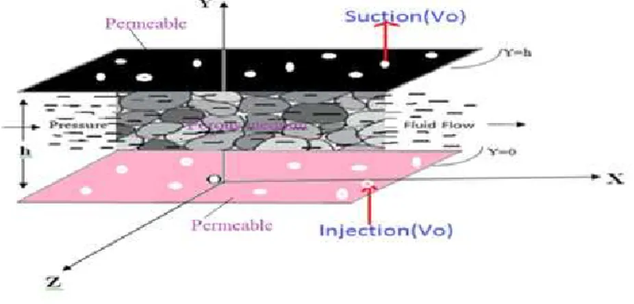
Consider the slow steady flow of a second order slightly thermo-viscous fluid through a porous medium bounded between two permeable parallel plates[See Fig. 1]. The flow in the absence of external body forces, internal heat source and the pressure gradient in the flow direction is examined. The motion of the upper plate, moving with a given velocityu0relative to the lower plate along the flow direction. With reference to a coordinate system O(XYZ) with origin on the fixed plate, the X-axis in the direction of the plate movement, Y-axis perpendicular to plates, the plates are represented by y=0 and y=h . Further the two plates are maintained at constant temperaturesθ0and θ1respectively.
Let the steady flow between the two permeable parallel plates is characterized by the velocity field[u(y),v0, 0]and temperature fieldθ(y). This choice of the velocity evidently satisfies the continuity equation.
Adopting the notation given in nomenclature, the basic equations characterizing the flow are the following:
Equation of motion in X-direction :
ρv0 ∂u
∂y =µ
∂2u ∂y2−α6
∂ θ ∂x
∂2θ ∂y2−
µ
k∗u (1)
Equation of motion in Y-direction :
0=µc ∂ ∂y
∂u
∂y
2
Fig. 1. Flow configuration
Equation of motion in Z-direction :
0=α8 ∂ ∂y ∂ u ∂y ∂ θ ∂y
+ρfz (3)
and the energy equation:
ρc
u∂ θ
∂x +v0
∂ θ ∂y
=µ ∂u
∂y
2
−α8 ∂ θ ∂x
∂u
∂y
∂ θ ∂y +k
∂2θ ∂y2+β3
∂ θ ∂x
∂2u ∂y2−
µ
k∗u
2 (4)
The boundary conditions are :
u=0,θ=θ0at y=0a n du=u0,θ=θ1at y=h (5)
It can be noted from the Eqs. (2) and (3) that a rectilinear motion between two parallel plates of a thermo-viscous fluid generates forcesρfy =−µc∂∂y
∂ u
∂y 2
in the Y-direction andρfz =−α8∂∂y ∂ u ∂y ∂ θ ∂y
in the Z-direction, such a force ofρfy is the normal stress noted by Reiner-Rivlin(1954) for visco-inelastic fluids, the forceρfz is thermo-mechanical viscous stress force generated perpendicular to both the flow direction and the Reiner-Rivlin normal stress. This is observed by Koh and Eringen(1963) for a second order thermo-viscous fluids. The generation of normal stress ρfy (proportional to the cross-viscosity coefficient µc ) is also observed by Lakshmana Rao and Bhatnagar(1957) who investigated the rectilinear flow of visco-inelastic fluid through non-circular ducts.
The following dimensional quantities are introduced to convert the above basic equations to the non-dimensional form.
Y =yh, U =ρµhu, u0=ρµh, U0=ρµhu0, T=θθ1−−θθ00, C2=
h
θ1−θ0
∂ θ ∂x
S=hk2∗, V =ρµhv0, pr=µkc, b3=ρβh32c, a6=α6ρ (θ1−θ0)2
µ2 , a1= µ
2
ρh2c(θ1−θ0)
where C2is dimensional temperature gradient which is assumed to be constant. Further , S is the non-dimensional Darcy’s porosity parameter and is the non-non-dimensional Suction/injection parameter.
In terms of these non-dimensional quantities , the equations of motion and energy reduce to the following:
Equation of motion in the X-direction:
V0
d U
d Y =
d2U d Y2−a6C2
d2T
d Y2−SU (6)
Equation of motion in the Y-direction :
0=µc
d d Y
d U
d Y
2
+ρFY (7)
Equation of motion in the Z-direction :
0=α8 d
d Y
d T
d Y d U d Y
+ρFZ (8)
and the energy equation :
U C2+V0
d T d Y =a1
d U
d Y
2
−a6C2
d T d Y
d U
d Y −SU
2
+b3C2
d2U
d Y2 + 1
pr
d2T
d Y2 (9)
The Eqs. (6) and (9) are non linear and coupled differential equations in terms of the velocity fieldU(Y)and the temperature fieldT(Y). The perturbation technique is most powerful and elegant method to get the solutions of these type of equations. Hence this technique is employed to obtain the solutions of equation of motion and energy together with the boundary conditions :
U(0) =0,U(1) =1 (10)
and
T(0) =0,T(1) =1 (11)
4.
Method of solution
The fluid is assumed to be slightly thermo-viscous in the sense that the interaction between the mechanical stress and thermal gradients (characterized by the coefficienta6) is of a lower order in magnitude compared to the magni-tude of viscous dissipation d Ud Y2, the non-Fourier heat transfer coefficientb3and the Darcy’sporosity parameter S ( i.e. terms containinga6in the momentum and energy balance equations taken to be smaller than the other terms in the energy equation ).
For a slightly thermo-viscous fluid (in the sense that is small) , the thermo-mechanical stress interaction coefficient is very small (i.e.a6<<1 ) and so the flow of the thermo-viscous fluid is a perturbation over a non-thermo viscous fluid. In such a case the velocity and temperature fields can be expressed as
U(Y) =U(0)(Y) +a6U(1)(Y) +a62U (2)(
Y) +... (12) and
T(Y) =T(0)(Y) +a6T(1)(Y) +a62T (2)(
Y) +... (13) witha6is the perturbation parameter. Substituting the Eqs. (12) and (13) in Eqs. (6) and (9) and collecting terms of like powers ofa6, we obtain the equations in the successive approximations.
4.1.
Basics or Zero order approximation
The Equations in this approximation
V0
d U(0)
d Y =
d2U(0)
d Y2 −SU
(0)
(14)
and
U(0)C2+V0
d T(0)
d Y =b3C2 d2U(0)
d Y2 +
1
pr
d2T(0)
d Y2 (15)
together with the boundary conditions :
U(0)(0) =0,U(0)(1) =1 (16)
and
T(0)(0) =0,T(0)(1) =1 (17)
From the Eq. (14) and using the boundary conditions in (16) the velocity distribution is obtained as
U(0)(Y) =em1(Y−1)s i n h m2(Y) s i n h m2
(18)
The Eq. (15) together with theEq. (18) and the boundary conditions (17) yields the temperature distribution
T(0)(Y) =e
V0prY−1
eV0pr−1
+(e
V0prY−eV0pr)(q 2−q3)
eV0pr−1
+(1−e
V0prY)em1(q
2em2−q3e−m2)
eV0pr−1
+(e
V0pr−1)em1Y(q
2em2Y−q3e−m2Y)
eV0pr−1 (19)
where
m1=
V0 υ,m2=
v u tV 2 0 υ + 4S
µ ,q2=
pre−m1C2(m1+m2)Cρ−b3(m1+m2)2
d1s i n h m2
andq3=
pre−m1C2(m1−m2)(Cρ−b3(m1−m2)2)
d2s i n h m2
here
4.2.
First order approximation
The Equations in this approximation
V0
d U(1)
d Y =
d2U(1)
d Y2 +C2
d2T(0)
d Y2 −SU
(1)
(20)
and
U(1)C2+V0
d T(1)
d Y =b3C2 d2U(1)
d Y2 +
1
pr
d2T(1)
d Y2 (21)
together with the boundary conditions :
U(1)(0) =0,U(1)(1) =1 (22)
and
T(1)(0) =0,T(1)(1) =1 (23)
In these equations,U(0)(Y)andT(0)(Y)are given by (18) and (19). The Eq. (20), (21) and the boundary conditions (21) yield the velocity distribution
U(1)(Y) = C2e
m1Yq
1 µs i n h m2(V0pr−m1)2
e(V0pr−m1)Ys i n h m
2−e(V0pr−m1 )
s i n h m2Y −s i n h m2Y −1
+ C2e
m1Y
2m2µs i n h m2
(q2em2−q3e−m2)(Y −1)s i n h m2Y (24)
where
q1=
(V0pr)2
(V0pr−1)s i n h m2
[s i n h m2+h1+h2]
here
h1=
pre−m1(m12+m22)
d1
andh2=
2prem2m1m2
d2
and the temperature distribution
T(1)(Y) = 1 d1(eV0pr−1)
(eV0prY −eV0pr)T
1+em1−m2(1−eV0prY)(T1+T2) +e(m1−m2)Y(eV0pr−1)(T1+T2Y)
+T2[2(m1−m2)−V0pr] d2
1(eV0pr−1)
(eV0prY−eV0pr) +em1−m2(1−eV0prY) +e(m1−m2)Y(eV0pr−1)
+ 1
d2(eV0pr−1)
(eV0prY −eV0pr)T
3+em1+m2(1−eV0prY)(T3+T4) +e(m1+m2)Y(eV0pr−1)(T3+T4Y)
+T4[2(m1+m2)−V0pr] d2
2(eV0pr−1)
(eV0prY−eV0pr) +em1+m2(1−eV0prY) +e(m1+m2)Y(eV0pr−1)
+ T5 V0pr
eV0pr(1−eV0prY)−Y eV0prY(1−eV0pr) (25)
which satisfy the boundary conditions in (23) where
T1=
prC22(Cρ−(m1−m2)2) 2µem1s i n h m2
q1(eV0pr−em1+m2)
(V0pr−m1)2−m22
+q2e
m1+m2+q
3em1−m2 2m2
+q3C2(m1−m2)
µm2
T2=
q3C2 2µm2
ρc prC2+ (m1−m2)2
T3=
prC22(Cρ−(m1+m2)2) 2µem1s i n h m2
q1(eV0pr−em1−m2)
(V0pr−m1)2−m22
+q2e
m1+m2+q
3em1−m2 2m2
+q2C2(m1+m2)
µm2
T4=
q2C2 2µm2
ρc prC2+ (m1+m2)2
andT5=
q1C2pr(ρc C2+V02pr) µ[(V0pr−m1)2−m22]
The velocity and temperature distribution up to the first order approximation is as follows:
The velocity distribution :
U(Y) =U(0)(Y) +a6U(1)(Y) and the temperature distribution :
T(Y) =T(0)(Y) +a6T(1)(Y)
Note: The variations of the velocity and temperature profiles for different values of the flow parameters are shown in the illustrations Fig.2- Fig.13.
5.
Results and discussion
The flow presented in this paper is investigated under the assumption of slow steady motion of a fluid so that the viscous dissipation , Darcy’sdissipation and thermo-mechanical stress interaction coefficient terms are neglected. The effects of various material parameters such as Strain thermal conductivity coefficient(b3), thermo-mechanical stress interaction coefficient(a6), Darcy’sporosity parameter(S) and the Suction/injection parameter(V0) on the ve-locity and temperature distributions have been illustrated for the fixed valuesC2=1 ,pr=1 anda1=1 .
The variations of velocity and temperature profiles for small values of Darcy’sporosity parameter(S) and the Suc-tion/injection parameter(V0) are shown in Fig. 2, Fig. 3, Fig. 4, Fig. 8, Fig. 9and Fig. 10and for large values of Darcy’sporosity parameter(S) and the Suction/injection parameter((V0) ) are shown in Fig.5, Fig.6, Fig. 7, Fig. 11, Fig.12and Fig.13.
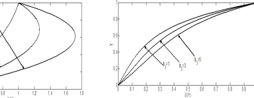
Fig. 2. Variations of the velocity profiles with S=1,V0=
0.1 ,a6=0.01 andb3
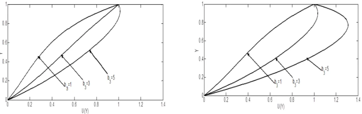
Fig. 3. Variations of the velocity profiles with S=1,V0=
0.1 ,a6=0.03 andb3
Fig. 4. Variations of the velocity profiles with S=1,V0=
0.1 ,a6=0.05 andb3
Fig. 5. Variations of the velocity profiles with S=10,V0=1
,a6=0.01 andb3
It is observed from the Fig. 2, Fig.3, Fig.4that, the velocity profiles raise towards the upper plate as the values of Strain thermal conductivity coefficient(b3) increases from 1 to 5. Fig.2shows that , for small value of Strain thermal conductivity coefficient(i.e. forb3=1), the straight line profile is realized and the maximum velocity attains at the upper plate. From the Fig.3, Fig.4, it is observed that , for large values of Strain thermal conductivity coefficient(i.e. forb3=3 ,5) the maximum velocity attains near the centre of the channel. Fig.2, Fig.3, Fig.4also shows that, as the value of thermo-mechanical stress interaction coefficient(a6) increases , the velocity profiles raise and the rate of raise of the velocity profiles for small value of (i.e. forb3=1) are very slow compared to the rate of raise of those for large values of ( i.e. forb3=3 , 5 ).
From the Fig.5, Fig.6, Fig.7, It is noticed that, as the value of thermo-mechanical stress interaction coefficient(a6) and Strain thermal conductivity coefficient(b3) both increases, the velocity profiles increase and coincide with the velocity of the upper plate. Fig.5indicate that , as the value of Strain thermal conductivity coefficient(b3) increases , the bending of the velocity profiles increase and attain the maximum velocity at the hotter plate.
Fig. 6. Variations of the velocity profiles with S=10,V0=1
,a6=0.03 andb3
Fig. 7. Variations of the velocity profiles with S=10,V0=1
,a6=0.05 andb3
Fig. 8. Variations of the Temperature profiles with S=1,
V0=0.1 ,a6=0.01 andb3
Fig. 9. Variations of the Temperature profiles with S=1,
V0=0.1 ,a6=0.03 andb3
Fig. 10. Variations of the Temperature profiles with S=1,
V0=0.1 ,a6=0.05 andb3
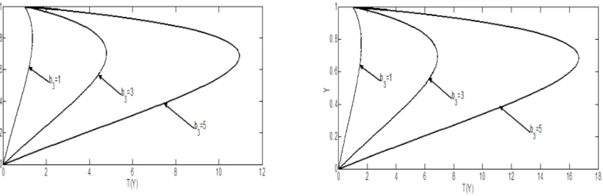
Fig. 11. Variations of the Temperature profiles with
S=10,V0=1 ,a6=0.01 andb3
hotter plate.
From the Fig. 11, Fig. 12and Fig. 13, It is noticed that, the temperature profiles increase faster as the value of Strain thermal conductivity coefficient(b3) increases from 1 to 5. For small value of Strain thermal conductivity coefficient( i.e. forb3=1 ), the rate of increase of temperature of the fluid is rather very slow while for large values of Strain thermal conductivity coefficient( i.e. forb3=3 ,5 ) , the rate of increase of the fluid temperature is very fast.
Fig. 12. Variations of the Temperature profiles with S=10,V0=1 ,a6=0.03 andb3
Fig. 13. Variations of the Temperature profiles with
S=10,V0=1 ,a6=0.05 andb3
Acknowledgements
The authors would like to thank different software companies (MatLab and LATEX) for developing the codes that help in the computation, verification of graphical results and editing the paper .
References
[1] S. L. Koh, A. C. Eringin, On the foundations of non-linear thermo-elastic fluids. Int.J. Engg. Scil. 1 (1963) 199 -229.
[2] B. D. Coleman, V. J. Mizel, On the existence of caloric equations of state, Journal of Chem.Phys. 40(1964) 1116-1125.
[3] A. E. Green, P. M. Naghdi, A dynamical theory of interacting Continua , Int.J. Engg. Sci. 3(1965) 231-241. [4] P. D. Kelly, Some viscometric flows of incompressible thermo-viscous fluids, Int. J. Engg. sci. 2(1965) 519-537. [5] P. Nageswara Rao, Some problems in thermo- Viscous fluid Dynamics, Ph. D thesis, K. U Warangal, 1979. [6] E. Nagaratnam, Some steady and unsteady flows of thermo- viscous fluids, Ph. D thesis, J.N.T.U Hyderabad,
2006.
[7] P. Nageswara Rao, N. Ch. Pattabhi Ramacharyulu , Steady flow of a second order thermo- viscous fluid over an infinite plate, Proc.Ind.Acad.Sci., 88A 2(1979) 157-162.
[8] W. E. Langlois, Steady flow of slightly visco-elastic fluid between rotating cylinders, Q.APP.Math. 1(1963) 61-71. [9] R. S. Rivlin, The solution of problems in second-order elasticity theory, J.Rat.Mech.Anal. 2(1954) 53-59. [10] N. Pandya, A. K. Shukla, Soret-Dufour and Radiation effect on unsteady MHD flow over an inclined porous plate
embedded in porous medium with viscous dissipation, Int. J. Adv. Appl. Math. and Mech. 2(1) (2014)107â ˘A¸S119. [11] M. S. Alam, M. Nurul Huda , A new approach for local similarity solutions of an unsteady hydromagnetic free convective heat transfer flow along a permeable flat surface, Int. J. Adv. Appl. Math. and Mech. 1(2) (2013) 39-52. [12] Ramesh Chand, Arvind Kumar, Thermal instability of rotating Maxwell visco-elastic fluid with variable gravity
in porous medium, Int. J. Adv. Appl. Math. and Mech. 1(2) (2013) 30-38.
[13] L. Preziosi, A. Farina, On Darcy’s Law for growing porous media, Int.J.Non-linear mechanics 37(2002) 485-491. [14] K. V. Yamamoto, Z. Yoshida, Flow through a porous wall with convective acceleration, Journal of Physical Society
3(1974) 774-779.
[15] G. S. Beaver, D. D. Joseph, Boundary conditions at a naturally permeable wall, J. Fluid Mechanism 30(1967) 197-207.
[16] Srinivas Joshi, P.Nageswar Rao and N.Ch. Pattabhi Ramacharyulu, Steady flow of thermo-viscous fluid between two parallel porous plates in relative motion, IEEMS 9(2010) 58-65.
[17] J. Bear, Dynamic of fluids in porous media, American Elsevier Pub.Co.inc., Newyork, 1970.
[18] R. E. Collis, Flow of fluids through porous materials, Reinhold publishing corporation, Newyork, 1961.