Impact of precipitation and land biophysical variables on the simulated discharge of European and Mediterranean rivers

(1)

HESSD

9, 5437–5486, 2012

Impact of precipitation and land

biophysical variables

C. Szczypta et al.

Title Page

Abstract Introduction

Conclusions References

Tables Figures

◭ ◮

Back Close

Full Screen / Esc

Printer-friendly Version Interactive Discussion

Discussion

P

a

per

|

Dis

cussion

P

a

per

|

Discussion

P

a

per

|

Discussio

n

P

a

per

|

Hydrol. Earth Syst. Sci. Discuss., 9, 5437–5486, 2012 www.hydrol-earth-syst-sci-discuss.net/9/5437/2012/ doi:10.5194/hessd-9-5437-2012

Hydrology and Earth System Sciences Discussions

This discussion paper is/has been under review for the journal Hydrology and Earth System Sciences (HESS). Please refer to the corresponding final paper in HESS if available.

Impact of precipitation and land

biophysical variables on the simulated

discharge of European and Mediterranean

rivers

C. Szczypta, B. Decharme, D. Carrer, J.-C. Calvet, S. Lafont, S. Somot, S. Faroux, and E. Martin

CNRM-GAME, M ´et ´eo-France, CNRS – URA1357, Toulouse, France

Received: 21 March 2012 – Accepted: 12 April 2012 – Published: 24 April 2012 Correspondence to: J.-C. Calvet (jean-christophe.calvet@meteo.fr)

(2)

HESSD

9, 5437–5486, 2012

C. Szczypta et al.

Title Page

Tables Figures

◭ ◮

Back Close

Full Screen / Esc

Discussion

P

a

per

|

Dis

cussion

P

a

per

|

Discussion

P

a

per

|

Discussio

n

P

a

per

|

Abstract

This study investigates the use of the ERA-Interim 3-hourly atmospheric reanalysis over Europe and the Mediterranean basin, to drive the ISBA-TRIP continental hydro-logical system, at a spatial resolution of 0.5◦, over the 1991–2008 period. Several versions of the representation of evapotranspiration in the ISBA land surface model

5

are used to simulate the runoff which is converted into river discharge by the TRIP river routing model. In particular, the impact of using contrasting representations of the vegetation variables is investigated: ISBA is used together with its upgraded carbon flux version (ISBA-A-gs). The latter is either driven by a satellite-derived climatology of the Leaf Area Index (LAI) or performs prognostic LAI simulations. As ERA-Interim

10

tends to underestimate precipitation, a number of precipitation corrections are pro-posed. In particular, the monthly GPCC precipitation product is used to un-bias the 3-hourly ERA-Interim estimates. This correction markedly improves the match between the ISBA-TRIP simulations and the river discharge observations of the Global Runo_ff Data Centre (GRDC), at 150 gauging stations. The interactive LAI version of ISBA-A-gs

15

does not perform as well as the original ISBA model at springtime. On the other hand, the use of the ISBA-A-gs model allows a better representation of river discharge at low water levels. Constraining the ISBA-A-gs LAI with satellite-derived LAI data improves the simulations at springtime.

1 Introduction

20

Over the last decades, Europe was affected by severe drought events. The drought of 2003 had a marked impact on agriculture and industry over Western and Central Europe (Vidal et al., 2010). In 2004 and in 2010, respectively, severe droughts af-fected the Iberian Peninsula (Gargia-Herrera et al., 2007) and Russia (Barriopedro et al., 2011). Drought duration and location are variable but always have economic,

so-25

(3)

HESSD

9, 5437–5486, 2012

C. Szczypta et al.

Title Page

Tables Figures

◭ ◮

Back Close

Full Screen / Esc

Discussion

P

a

per

|

Dis

cussion

P

a

per

|

Discussion

P

a

per

|

Discussio

n

P

a

per

|

understand these events and to predict when and where they will occur. Even if no uni-versally accepted definition of drought exist (Tate and Gustard, 2000), three consistent drought categories are frequently used and have been defined by Wilhite and Glantz (1985): meteorological drought (deficit in precipitation), agricultural drought (deficit in soil moisture, and/or in Leaf Area Index – LAI) and hydrological drought (deficit in river

5

discharge, groundwater storage). Modeling platforms including Land Surface Models (LSMs), forced by gridded atmospheric variables and coupled to runoff models, rep-resent e_fficient and powerful tools to understand the global hydrological cycle and to study different drought types. Indeed, while precipitation data allow the evaluation of meteorological droughts, LSMs coupled to runoff models are needed to

character-10

ize agricultural and hydrological droughts, with simulated biophysical variables (LAI, surface and root-zone soil moisture) fully consistent with surface flux (latent and sen-sible heat fluxes, CO2 fluxes) and river discharge simulations. Indeed, the LSM

per-formance impacts the hydrological simulations (Lhomann et al., 1998; Boone et al., 2004; Decharme 2007; Balsamo et al., 2009). LSMs were significantly improved over

15

recent decades and can now be coupled with river routing schemes to understand the regional and global water cycles (D ümenil and Todini, 1992; Habets et al., 1999; Oki et al., 1999; Decharme et al., 2006). Because the Mediterranean basin will proba-bly be affected by climate change to a large extent (Gibelin and D équ é, 2003; Giorgi, 2006; Planton et al., 2012), it is important to build monitoring systems of the land

sur-20

face variables and of the hydrological variables over this region. In the framework of the HYMEX (HYdrological cycle in the Mediterranean EXperiment) project (HYMEX White Book, 2008) and particularly with the aim of simulating hydrological droughts over the 1991–2008 period, river discharge simulations were performed with the ISBA (Interactions between Soil Biosphere and Atmosphere) LSM (Noilhan and Planton,

25

(4)

HESSD

9, 5437–5486, 2012

C. Szczypta et al.

Title Page

Tables Figures

◭ ◮

Back Close

Full Screen / Esc

Discussion

P

a

per

|

Dis

cussion

P

a

per

|

Discussion

P

a

per

|

Discussio

n

P

a

per

|

gridded atmospheric reanalysis (Simmons et al., 2007) was used to drive the coupled ISBA-TRIP continental hydrological system.

The river discharge simulated by ISBA-TRIP system results from the following water fluxes: (1) the ERA-I precipitation, (2) the simulated soil moisture changes, evapo-transpiration, and surface runoff and drainage. Therefore, provided unbiased

precip-5

itation data are used (Fekete et al., 2003), the simulated river flow can be used for the verification of the LSM simulations (Boone et al., 2004). Szczypta et al. (2011) have shown that, over France, the ERA-I precipitation correlates very well with the SAFRAN (Syst `eme d’Analyse Fournissant des Renseignements A la Neige) analysis (Quintana-Segui et al., 2008) based on in situ observations. However, ERA-I tends to

10

markedly underestimate the precipitation, by 27 % on average. Photiadou et al. (2011) have shown that the underestimated ERA-I precipitation leads to underestimated river discharges.

This study investigates to what extent the ERA-I precipitation bias can be reduced, and whether continental scale ISBA-TRIP simulations can be used to benchmark

sev-15

eral versions of the ISBA model.

In a first stage, the ERA-I precipitation bias is characterized over Europe and the Mediterranean basin, by comparing monthly ERA-I precipitation data with the monthly Global Precipitation Climatology Centre (GPCC) product (Rudolf et al., 2005), which is partly based on ground observations. The GPCC data are used to un-bias the ERA-I

20

3-hourly precipitation. The original and the unbiased ERA-I precipitation data sets are used by ISBA-TRIP to produce river discharge simulations. Following Decharme and Douville (2006b), the comparison between these simulations and the Global Runo_ff Data Centre (GRDC) daily observations is used to assess the added value of the unbi-ased ERA-I precipitation on the ISBA-TRIP simulations.

25

In a second stage, the relevance of using di_fferent precipitation fields and versions of ISBA LSM (the standard version or the CO2-responsive versions) is examined through

(5)

HESSD

9, 5437–5486, 2012

C. Szczypta et al.

Title Page

Tables Figures

◭ ◮

Back Close

Full Screen / Esc

Discussion

P

a

per

|

Dis

cussion

P

a

per

|

Discussion

P

a

per

|

Discussio

n

P

a

per

|

standard version and the ISBA-A-gs carbon version (Calvet et al., 1998; Gibelin et al., 2006). The latter uses either the same satellite-derived LAI climatology as the standard ISBA or produces prognostic LAI estimates. The impact of these LSM options and of LAI on the river discharge simulations is evaluated. After an overview of the different data sets, models, scores and methods used in this study (Sect. 2), the results are

5

presented in Sect. 3. The impact of precipitation on the runoffmodel simulations over Europe is presented, together with the impact of the carbon option of ISBA and LAI. These results are analyzed and discussed in Sect. 4, in relation to the water balance of the Mediterranean basin. The main conclusions of this study are summarized in Sect. 5.

10

2 Data and methods

This section presents the different data sets, the models used to simulate land bio-physical variables, surface fluxes and river discharge, and the modeling protocol. The method used to un-bias the ERA-I precipitation is presented.

2.1 Meteorological variables

15

The ERA-I atmospheric reanalysis is used in this study to drive the coupled ISBA-TRIP model over the 1991–2008 period, at a spatial resolution of 0.5◦, corresponding to 8142 land grid cells over the considered area (see Fig. 1).

2.1.1 The ERA-I reanalysis

The ECMWF ERA-I reanalysis covers dates from 1 January 1979 and is updated in

20

(6)

HESSD

9, 5437–5486, 2012

C. Szczypta et al.

Title Page

Tables Figures

◭ ◮

Back Close

Full Screen / Esc

Discussion

P

a

per

|

Dis

cussion

P

a

per

|

Discussion

P

a

per

|

Discussio

n

P

a

per

|

while producing a forecast, the atmospheric model simulates a large variety of physical variables such as precipitation, turbulent fluxes, radiation fields, and cloud properties. Even if these quantities are not directly observed, they are constrained by the obser-vations used to initialize the forecast. All these forcing data were projected from the original reduced Gaussian grid (of about 0.7◦×0.7◦) to a 0.5◦×0.5◦ grid, at a 3-hourly

5

time step. A full description of the data can be found in Simmons et al. (2007) and the assimilation system is described in Dee et al. (2011). A verification of the different ERA-I atmospheric variables was performed over France by Szczypta et al. (2011). They found that, on average, the ERA-I precipitation is underestimated by 27 %, in comparison to the SAFRAN reference analysis, based on thousands of rain gauges.

10

A scale-selective rescaling procedure correcting for the ERA-I 3-hourly precipitation bias was implemented by ECMWF (Balsamo et al., 2010), based on the monthly accu-mulated precipitation provided by the Global Precipitation Climatology Project (GPCP). The GPCP v2.1 product (Hu_ffman et al., 2009) is a monthly global climatology gen-erated on a 2.5◦×2.5◦ grid and available over the 1979–2009 period. This data set

15

is a merged product combining various observations related to precipitation, includ-ing satellite observations and rain gauge data, assembled and analyzed by the Global Precipitation Climatology Centre (GPCC, Rudolf et al., 2010) and by the Climate Pre-diction Center of the National Oceanic and Atmospheric Administration (NOAA). Note that GPCP v2.1 is an improved version of GPCP v2.0, described in Adler et al. (2003).

20

Hereafter, the GPCP rescaled ERA-I precipitation will be referred to as ERA-I-R. The GPCC provides a global monthly precipitation analysis at a 0.5◦×0.5◦resolution (GPCC v5) over the 1901–2010 period (Becker, 2011). The GPCC database com-prises monthly quality-controlled precipitation totals from more than 70 000 rain gauge stations worldwide (Fuchs et al., 2009). The GPCC network is relatively dense in

Eu-25

(7)

HESSD

9, 5437–5486, 2012

C. Szczypta et al.

Title Page

Tables Figures

◭ ◮

Back Close

Full Screen / Esc

Discussion

P

a

per

|

Dis

cussion

P

a

per

|

Discussion

P

a

per

|

Discussio

n

P

a

per

|

2.1.2 Unbiased ERA-I precipitation based on the GPCC monthly product

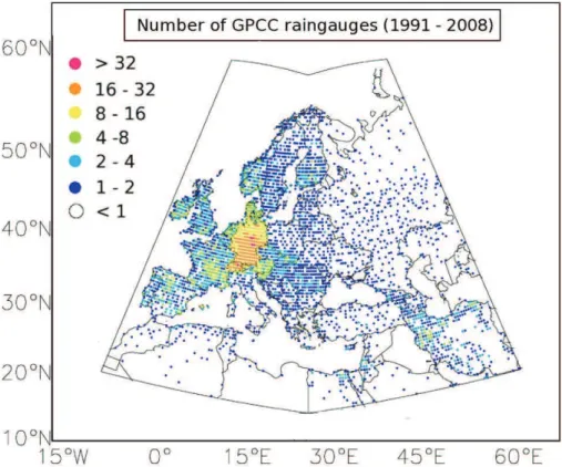
The GPCC monthly precipitation product is based, to a large extent, on ground ob-servations, and its quality depends on the density of rain gauges used to prepare the product. Figure 1 presents the mean number of rain gauges per grid cell (0.5◦×0.5◦) used to generate the GPCC precipitation data set in the area considered in this study,

5

over the 1991–2008 period. Over the considered area, 11 263 rain gauges are used. While many rain gauges are used in Europe (especially in Germany), large parts of Russia, North Africa, Turkey, and of the Middle-East present a low density of in situ observations. In this study, this product is used to perform a correction of the system-atic biases in the ERA-I and ERA-I-R 3-hourly reanalyses. The ERA-I and ERA-I-R

10

3-hourly spatial and temporal distribution of precipitation is preserved, while the biases with the monthly GPCC climatology are reduced. The hybridization of the two data sets with GPCC is performed as in Decharme and Douville (2006b):

P_hybrid3 h =P_ERA-I3 h ×P_GPCCmonth/P_ERA-Imonth. (1) Hereafter, the unbiased ERA-I and the ERA-I-R precipitation based on the GPCC

15

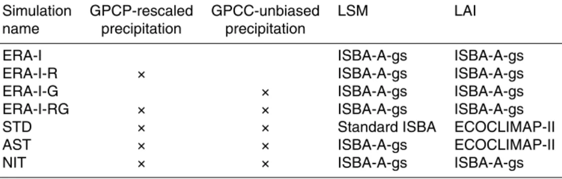
monthly product is referred to as ERA-I-G and ERA-I-RG, respectively (see Table 1).

2.2 The GRDC river discharge data base

The Global RunoffData Center (GRDC, Koblenz, Germany) database is collection of river discharge data at a daily or monthly time steps, from more than 8000 stations worldwide. In this study, the GRDC daily data are selected over the domain presented

20

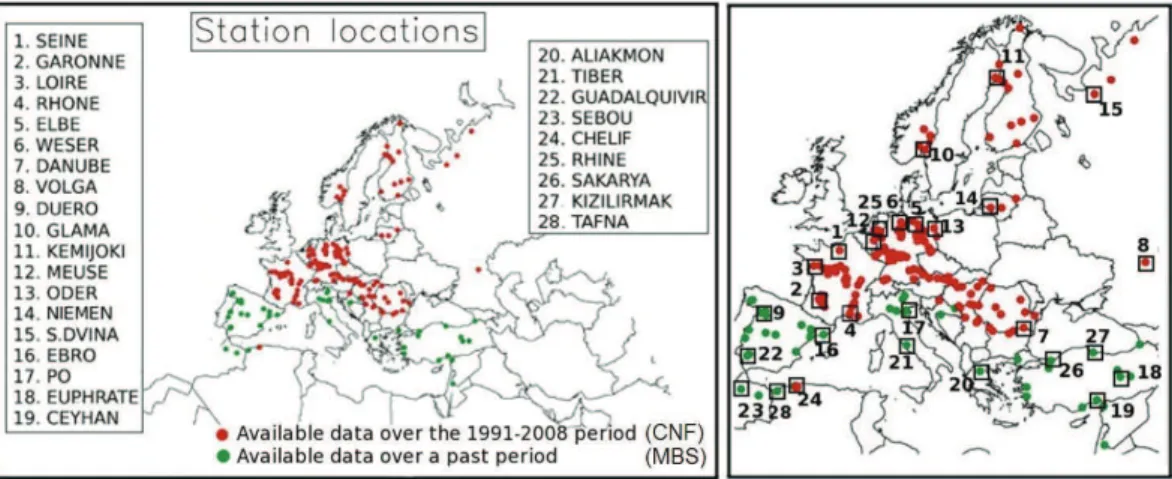
in Fig. 1, for the 1991–2008 period, for sub-basins with drainage areas of at least 10 000 km2 and with a minimum observed period of 5 yr. This results in 150 gauging stations, mainly located in Central, Eastern and Northen Europe and in France (here-after referred to as “CNF”), as shown by Fig. 2 (red dots). Only one of these stations is located in North Africa (Algeria). For Southern Europe, the Middle-East, and North

25

(8)

HESSD

9, 5437–5486, 2012

C. Szczypta et al.

Title Page

Tables Figures

◭ ◮

Back Close

Full Screen / Esc

Discussion

P

a

per

|

Dis

cussion

P

a

per

|

Discussion

P

a

per

|

Discussio

n

P

a

per

|

referred to as “MBS”), GRDC data from 46 gauging stations are available over a past period (Fig. 2). The first time series starts in 1912 and for these stations, no data is available after 1994. Moreover, about half of the time series are available at a monthly time step, only. Therefore, the MBS stations are used in this study to build a monthly climatology. Only sub-basins with drainage areas of at least 5000 km2 and with a

min-5

imum observation period of 10 yr are considered, except for the time series of the Po basin in Italy, which covers a 6-yr period (1980–1985), only.

2.3 The SURFEX modeling platform

The SURFEX (SURFace EXternalis ´ee) modeling platform (Le Moigne et al., 2009) includes the ISBA and the ISBA-A-gs LSMs, coupled with the TRIP river routing model.

10

The LSMs simulate soil moisture and the associated surface runoffand deep drainage. The latter two variables are used by TRIP for the simulation of river flow.

2.3.1 The ISBA LSM

The ISBA LSM (Noilhan and Planton, 1989) was developed at M ´et ´eo-France to de-scribe the land surface processes in weather forecast and climate models. ISBA uses

15

a limited number of parameters, mapped according to the soil and vegetation types provided by the global 1 km×1 km resolution ECOCLIMAP land cover and look-up ta-ble database (Masson et al., 2003). ISBA uses the force-restore method of Deardoff (1977, 1978) to calculate the time variation of the surface energy and water budgets (Noilhan and Planton, 1989). The soil hydrology is represented by three layers: a thin

20

surface layer with a uniform depth, a root-zone layer, and a deep soil layer (Boone et al., 1999) contributing to evaporation through capillarity rises. Also, the model sim-ulates the water interception storage, and the snow pack evolution based on a simple one-layer scheme (Douville et al., 1995). The deep drainage is computed according to Noilhan and Mahfouf (1996).

(9)

HESSD

9, 5437–5486, 2012

C. Szczypta et al.

Title Page

Tables Figures

◭ ◮

Back Close

Full Screen / Esc

Discussion

P

a

per

|

Dis

cussion

P

a

per

|

Discussion

P

a

per

|

Discussio

n

P

a

per

|

ISBA also includes a comprehensive parameterization of sub-grid hydrology to ac-count for the heterogeneity of precipitation, infiltration, topography and vegetation within each grid cell. A TOPMODEL approach (Beven and Kirkby, 1979) has been used to simulate a saturated fraction where precipitation is entirely converted into surface runoff(Decharme et al., 2006). Infiltration over frozen and unfrozen soils is computed

5

via two sub-grid exponential distributions of rainfall intensity and soil maximum infiltra-tion capacity. Finally, a tile approach, in which each grid cell is divided into a series of sub-grid patches, is used to represent land cover and soil depth heterogeneities. Distinct energy and water budgets are computed for each tile within a grid cell and the relative fractional coverage of each surface type is used to determine the grid-cell

10

average of the various output variables. More details can be found in Decharme and Douville (2006a). The stomatal resistance of the vegetation is computed with a mul-tiplicative model based on Jarvis (1976), where a minimum stomatal resistance is di-vided by stress functions representing the e_ffect of solar radiation, soil moisture stress, air humidity and air temperature.

15

2.3.2 The ISBA-A-gs LSM

On the basis of ISBA, Calvet et al. (1998) developed ISBA-A-gs, which is a CO₂ -responsive version of ISBA. This model accounts for photosynthesis and its coupling with stomatal conductance at the leaf level. The vegetation net assimilation is com-puted and used as an input to a simple growth sub-model able to predict LAI (Calvet

20

and Soussana, 2001). The model also includes an original representation of the soil moisture stress. Two different types of the plant response to drought are distinguished, for both herbaceous vegetation (Calvet, 2000) and forests (Calvet et al., 2004). The plant response to drought is characterized by the evolution of the water use e_fficiency (WUE) under moderate stress: WUE increases in the early soil water stress stages in

25

(10)

HESSD

9, 5437–5486, 2012

C. Szczypta et al.

Title Page

Tables Figures

◭ ◮

Back Close

Full Screen / Esc

Discussion

P

a

per

|

Dis

cussion

P

a

per

|

Discussion

P

a

per

|

Discussio

n

P

a

per

|

under various environmental conditions. As for ISBA, it is possible to drive ISBA-A-gs with the ECOCLIMAP seasonal LAI climatology.

2.3.3 The TRIP hydrological model

TRIP was developed at the Tokyo University by Oki and Sud (1998) and was recently coupled to the SURFEX system. TRIP converts the daily runoffsimulated by ISBA or

5

ISBA-A-gs into river discharges. It is a simple linear model based on a two prognostic equation for the water mass within each grid cell of the hydrological network (Decharme et al., 2010). TRIP takes into account a simple groundwater reservoir which can be seen as a simple soil-water storage and a variable stream flow velocity as proposed by Arora and Boer (1999). More details about these parameterizations can be found in

10

Decharme et al. (2010).

2.3.4 Experimental design

The simulations performed in this study are produced by SURFEX version 6.2. SUR-FEX is driven by the 3-hourly meteorological data described in Sect. 2.1, for the 1991– 2008 period, at a 0.5◦grid resolution. The year 1991 is run three times in order to

spin-15

up the simulations. The simulations are based on the ECOCLIMAP-II (Faroux et al., 2009) land cover map. Hereafter, the simulations performed by the standard version of ISBA are referred to as “STD” (see Table 1). ISBA-A-gs is used in the two following configurations (Table 1):

– the annual cycle of LAI is provided by ECOCLIMAP-II as a fixed satellite-derived

20

climatology, as for STD simulations. This simulation is referred to as “AST” (A-gs and the enhanced soil moisture stress option).

– ISBA-A-gs simulates daily LAI values. This simulation is referred to as “NIT” (with a nitrogen-dilution based representation of leaf biomass, in addition to the AST capability).

(11)

HESSD

9, 5437–5486, 2012

C. Szczypta et al.

Title Page

Tables Figures

◭ ◮

Back Close

Full Screen / Esc

Discussion

P

a

per

|

Dis

cussion

P

a

per

|

Discussion

P

a

per

|

Discussio

n

P

a

per

|

The used global river channel network of the ISBA-TRIP model has a spatial resolu-tion of 0.5◦×0.5◦resolution. The comparison between AST-TRIP and NIT-TRIP permits to assess to what extent differences in the seasonal and interannual variability of LAI impacts the river discharge simulations. Indeed, the same representation of biophys-ical processes, and the same tiling approach are used in AST and NIT simulations,

5

except for constrained and unconstrained LAI. On the other hand, the comparison be-tween STD-TRIP and AST-TRIP permits the benchmarking of ISBA and ISBA-A-gs evapotranspiration fluxes, because the two simulations use the same LAI climatology and the same tiling approach. As a component of the hydrological cycle, evapotran-spiration influences the soil moisture dynamics and the water flux from the LSM to the

10

TRIP river routing scheme. Therefore, while comparing the GRDC observations with the TRIP river discharge simulations forced by STD and AST permit the assessment of the contrasting transpiration parameterization used in ISBA and in ISBA-A-gs, the use of NIT allows the evaluation of the interactive LAI simulated by ISBA-A-gs.

2.4 Comparison between observed and simulated river discharges

15

In this study, river discharge simulations are obtained from (1) NIT-TRIP driven by the four different precipitation data sets (ERA-I, ERA-I-R, ERA-I-G, ERA-I-RG) described in Sect. 2.1.2, (2) STD-, AST-, NIT-TRIP driven by ERA-I-RG. The simulations are com-pared with the available GRDC river discharge observations.

The comparison of the various precipitation data sets permits the determination of:

20

– the precipitation impact on the river discharge simulations (a model sensitivity study)

– the best precipitation data set to drive the coupled LSM-TRIP model

– the usefulness of rescaling ERA-I twice (first with GPCP and second with GPCC) vs. rescaling ERA-I once with GPCC.

(12)

HESSD

9, 5437–5486, 2012

C. Szczypta et al.

Title Page

Tables Figures

◭ ◮

Back Close

Full Screen / Esc

Discussion

P

a

per

|

Dis

cussion

P

a

per

|

Discussion

P

a

per

|

Discussio

n

P

a

per

|

Observed and simulated river discharge (Q) data are generally expressed in m3s−1. As the observed drainage area may differ slightly from the simulated one, scaled Q

values in mm d−1 (the ratio ofQ to the drainage area) are used in this study. The use of mm d−1units forQvalues, permits the direct comparison ofQwith precipitation and evaporation values, both expressed in mm d−1.

5

Di_fferent hydrological skill scores (Krause et al., 2005) can be used in order to assess to what extent the simulations are close to the GRDC observations. Four scores are used in this study:

– the annual discharge ratio criterion, the Qsim/Qobs ratio, where Qsim and Qobs

represent the mean simulated and observed river discharges, respectively,

10

– the root mean square difference (RMSD) between GRDC observations and the simulatedQvalues, based on scaled monthly anomalies (dimensionless),

– the square correlation coefficient (r2), based on daily time series,

– the efficiency skill score (Eff) defined as the Nash criterion (Nash and Sutcliff, 1970) that measures the model ability to capture the daily discharge dynamics.

15

The latter is defined as:

E_{ff =}1− P

(Qsim(t)−Qobs(t)) 2 P

(Qobs(t)−Qobs)2

(2)

whereQobsrepresents the observed meanQvalue. The best Effvalue is 1, for a perfect

simulation. The Eff coefficient can be negative if the simulatedQ is very poor and is above 0.5 for a fair simulation (Boone et al., 2004; Decharme et al., 2006).

20

The scaledQanomalies used in the computation of the RMSD score are defined as:

Ano(mo,yr)=Q(mo,yr)−avg(Q(mo, :))

(13)

HESSD

9, 5437–5486, 2012

C. Szczypta et al.

Title Page

Tables Figures

◭ ◮

Back Close

Full Screen / Esc

Discussion

P

a

per

|

Dis

cussion

P

a

per

|

Discussion

P

a

per

|

Discussio

n

P

a

per

|

where Ano(mo,yr) andQ(mo,yr) are, respectively, the anomaly and theQfor the month mo and the year yr; avg(Q(mo, :)) and stdev(Q(mo, :)) are the average and the standard deviation of theQof the month mo, for all years, respectively.

The various ISBA-TRIP simulations can be compared using average score values and their range. As the statistical distribution of the scores may di_ffer from one

simula-5

tion to another, and across stations, the analysis of the cumulative distribution functions (CDF) of the scores is useful, also. Finally, the seasonal changes in the performance of a given simulation can be assessed by calculating the scores month by month, across the 18 yr, and the fraction of stations presenting a score value within a predefined range. In this study, we used [0.5,1] and [0.8,1.2] for Effand Qsim/Qobs, respectively. 10

The monthly scores of the stations are determined using a moving window of three months. The number of daily Q values used in the calculation of the monthly scores varies from 1602 to 1656. It must be noted that all the scores are based on daily values, except for RMSD, based on monthly values.

3 Results

15

This section presents the impact of using different (1) precipitation fields and (2) ver-sions of the ISBA LSM, on the quality of the river discharge simulations of ISBA-TRIP over the CNF domain for the 1991–2008 period. The climatology covering the MBS is used in the Discussion Sect. 4.

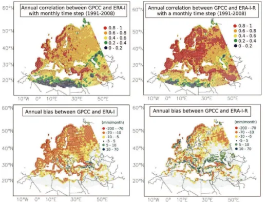
3.1 Correction of ERA-I precipitation

20

Figure 3 shows a comparison of the original monthly ERA-I and ERA-I-R precipita-tion estimates with the GPCC monthly data product, in terms of bias and temporal correlation. Ther2score calculation is based on 216 monthly precipitation values cor-responding to the 1991–2008 period. The correlation between ERA-I and GPCC is good (r2>0.6) over a large part of Europe and poor or non-significant around the

(14)

HESSD

9, 5437–5486, 2012

C. Szczypta et al.

Title Page

Tables Figures

◭ ◮

Back Close

Full Screen / Esc

Discussion

P

a

per

|

Dis

cussion

P

a

per

|

Discussion

P

a

per

|

Discussio

n

P

a

per

|

Caspian Sea, and (at the south of the domain) from the Sahara arid areas to Irak. ERA-I-R correlates better with the GPCC monthly product than the initial ERA-I pre-cipitation for a large part of the considered area and particularly over Europe. Very good (r2>0.8) correlations are obtained over a large part of the domain. The r2 val-ues tend to decrease in coastal areas, and while good correlations are observed over

5

the Middle-East and in North Africa, non-significant correlations are still obtained close to the Caspian Sea and in the Sahara desert where precipitation is close to zero.

Regarding the biases, the GPCP rescaling of ERA-I-R tends to increase the precip-itation values, thus reducing the marked precipprecip-itation underestimation of ERA-I. Over the whole domain, the underestimation decreases from about 20 % for ERA-I to 6 % for

10

ERA-I-R. However, the relative increase in the ERA-I-R precipitation, relative to ERA-I, is excessive for some coastal regions, where a marked overestimation of the precip-itation is observed. In Northern Europe, and in a number of mountainous areas (the Pyrenees, the Alps, the French Massif Central, the Carpathians, the Caucasus Moun-tains), the ERA-I-R precipitation is still underestimated in comparison to the monthly

15

GPCC product. It must be noted that the hybrid 3-hourly ERA-I-G and ERA-I-RG prod-ucts are based on the GPCC monthly data (through Eq. 1) and as such are completely unbiased and perfectly correlated with GPCC, on a monthly basis. However, the 3-hourly precipitation temporal distributions of ERA-I-G and ERA-I-RG differ slightly. In the following section, the impact of di_fferences in the precipitation forcing on the Q

20

simulations of the coupled ISBA-A-gs/TRIP model is investigated.

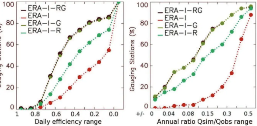
3.2 Impact of precipitation on the simulated CNF river discharge

The verification of the daily discharge simulations is based on the 150 GRDC stations of the CNF domain. Figure 4 presents the CDFs of the Eff score and of the depar-ture of the Qsim/Qobs ratio from 1, for the NIT-TRIP simulations forced by ERA-I and 25

(15)

HESSD

9, 5437–5486, 2012

C. Szczypta et al.

Title Page

Tables Figures

◭ ◮

Back Close

Full Screen / Esc

Discussion

P

a

per

|

Dis

cussion

P

a

per

|

Discussion

P

a

per

|

Discussio

n

P

a

per

|

For ERA-I, ERA-I-R, ERA-I-G, and ERA-I-RG, the fractions of the 150 CNF GRDC stations presenting a Eff score greater than 0.5 are 11 %, 30 %, 50 % and 52 %, re-spectively. Similar results are found (not shown) using STD-TRIP or AST-TRIP instead of NIT-TRIP. Overall, the ERA-I-RG simulations provide the best results, and the ISBA-TRIP simulations described below are all based on the ERA-I-RG precipitation data.

5

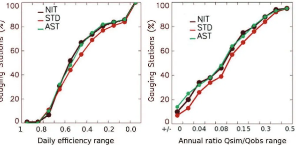
3.3 Impact of changes in the LSM configuration on the simulated CNF river

discharge

In this section, the simulatedQvalues obtained with different versions of the ISBA LSM are compared to GRDC gauging measurements. Figure 5 presents the CDFs of the Eff score and of the departure of theQsim/Qobs ratio from 1, for the NIT-, STD- and AST-10

TRIP simulations. The NIT curves of Fig. 5 correspond to the same simulation as the ERA-I-RG curves of Fig. 4 (Table 1). Ther2 and RMSD CDFs are not shown in Fig. 5 since the NIT, STD, and AST curves are almost confounded (see the corresponding scores in Table 2). The E_ffandQsim/QobsCDFs present more variability, and show that

the NIT- and AST-TRIP simulations perform better than STD-TRIP.

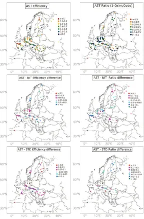
15

Figure 6 shows the spatial distribution of the AST-TRIP Eff score and of the diff er-ences between AST-TRIP and the two other simulations over the entire 1991–2008 period. Values of the Effscore better than 0.5 are obtained for a large fraction of the 150 stations: 44 %, 52 %, and 49 % for STD, NIT, and AST, respectively. Inadequate simulations, characterized by negative E_ff values, are obtained for 16 %, 13 %, and

20

13 % of the stations, respectively. For many regions, STD, AST and NIT present sim-ilar Eff scores. While NIT presents the best Effscores over Scandinavia, AST tends to outperform NIT in other regions, for 19 % of the stations (especially in France and in Germany). The AST simulations outperform STD simulations more extensively, for 40 % of the stations (e.g. in Scandinavia, in the Danube basin), while the reverse is true

25

(16)

HESSD

9, 5437–5486, 2012

C. Szczypta et al.

Title Page

Tables Figures

◭ ◮

Back Close

Full Screen / Esc

Discussion

P

a

per

|

Dis

cussion

P

a

per

|

Discussion

P

a

per

|

Discussio

n

P

a

per

|

Also, Fig. 6 presents, the departure of theQsim/Qobs ratio from 1 for the AST-TRIP

simulations and the di_fferences between AST-TRIP and the other simulations. While a majority of stations (63 %, 61 % and 57 % for AST, NIT and STD, respectively) present a good score (0.85< Qsim/Qobs<1.15), a significant fraction of the stations (18 %,

19 % and 24 %, respectively) do not perform well (Q_sim/Q_obs<0.7 orQ_sim/Q_obs>1.3).

5

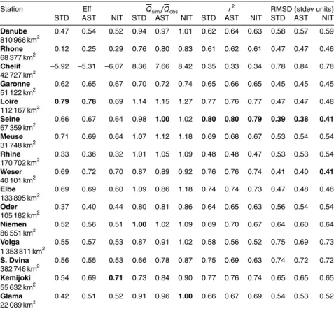
Consistent with the E_ffcriterion, AST tends to performs better than NIT in France and in Germany, and better than STD in Scandinavia. For all the model versions, the median RMSD value is 0.57 (Table 2). The 10 % and 90 % percentile values are 0.47 and 0.80, respectively. The stations presenting RMSD values higher than 0.8 are found in France, at the upstream of the Garonne, Loire, and Rhone rivers, in Scandinavia, and

10

in Algeria.

Figure 7 shows the mean monthly values of the observed and simulatedQ values for the downstream of the largest CNF basins (>20 000 km2). In the case of the Rhone river, the Viviers station is used instead of the downstream Beaucaire station as there is a great deal of water extraction between Viviers and Beaucaire. Also, the Durance

15

river, is a major tributary of the Rhone upstream Beaucaire and is markedly influenced by dams (Boone et al., 2004).

The Russian Pechora and Mezen rivers are not shown because they present results very similar to those obtained for the Severnaya Dvina river. Table 2 details the different scores (Eff, ratioQsim/Qobs,r

2

, RMSD) of the STD, AST, and NIT simulations for the

20

16 rivers of Fig. 7. Figure 7 shows that, in general, ERA-I tends to underestimateQ, except for the Chelif station (Algeria), which is influenced by dams. On the other hand, NIT tends to simulate the largestQvalues, during all seasons. At low water levels, STD produces the lowestQvalues. Table 2 shows that the RMSD andr2scores do not vary much from one version of the LSM to another. The differences in RMSD values between

25

(17)

HESSD

9, 5437–5486, 2012

C. Szczypta et al.

Title Page

Tables Figures

◭ ◮

Back Close

Full Screen / Esc

Discussion

P

a

per

|

Dis

cussion

P

a

per

|

Discussion

P

a

per

|

Discussio

n

P

a

per

|

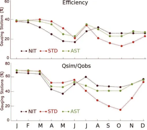
As Fig. 7 and Table 2 show that the Effand Qsim/Qobs scores respond to changes

in LSM and that the quality of the simulations may vary from one season to another, a seasonal analysis was performed using all the CNF stations. These scores are also presented in Fig. 8 on a monthly basis for a moving window of three months in order to highlight the seasonal features. It is shown that the performance of a given simulation

5

with respect to the others varies from one month to another. In March-April-May, STD presents good Effand Qsim/Qobs scores for a larger fraction of stations than the AST

and NIT simulations. For example, in May, STD, AST, and NIT present Effvalues higher than 0.5 for 36 %, 24 %, and 19 % of the stations, respectively. This indicates that, at springtime, the unconstrained representation of LAI in NIT-TRIP is detrimental to the

10

river discharge simulation, and has more impact than differences in the calculation of plant transpiration. The opposite result is obtained from August to October, with STD and NIT presenting the poorest and the best E_ffvalues, respectively. Also, AST performs nearly as well as NIT during this period of the year, indicating that, during the autumn, the calculation of plant transpiration in STD is detrimental to the river discharge

15

simulation, and has more impact than differences in LAI. TheQsim/Qobs ratio score is

particularly good for NIT, from August to December, with about 50 % of the stations presenting aQsim/Qobs ratio close to one, against about 30 % or less for STD-TRIP.

Figures 9 and 10 present the seasonal distribution of differences in Eff scores, in terms of maps and scatter plots, respectively. The differences are shown for three

20

periods, corresponding to the March-April-May, June-July-August, and September-October-November 3-monthly windows in Fig. 8, and for three model pairs: AST vs. STD, AST vs. NIT, and NIT vs. STD. Since AST and STD share the same representa-tion of LAI (derived from ECOCLIMAP-II), the differences between AST and STD permit to identify in Fig. 9 the regions where changes in the description of the transpiration

pro-25

(18)

HESSD

9, 5437–5486, 2012

C. Szczypta et al.

Title Page

Tables Figures

◭ ◮

Back Close

Full Screen / Esc

Discussion

P

a

per

|

Dis

cussion

P

a

per

|

Discussion

P

a

per

|

Discussio

n

P

a

per

|

assess how the LAI values impact theQsimulations. More often than not, the impact of constraining LAI with ECOCLIMAP-II is either moderate or changes (from positive to negative or vice versa) from one period to another. For the French Loire stations and one Garonne station, AST presents systematically better results than NIT. On the other hand, NIT always outperforms AST in Norway. While NIT tends to outperform STD in

5

July and October, the reverse is true in April. For the French Loire and Garonne sta-tions, STD presents systematically better results than NIT, across seasons. For a given river gauging station, Fig. 10 shows both the E_ffscore values and their di_fferences from one simulation to another. This permits the analysis of the impact of the quality of the simulations on the Effdifferences. In general, the few stations presenting the best Eff

10

scores do not present marked di_fferences from one simulation to another. Figure 10 shows that AST and NIT tend to systematically outperform STD during the autumn.

3.4 Impact of changes in the LSM configuration on the simulated MBS river

discharge

The monitoring of hydrological drought events over Mediterranean regions is more

chal-15

lenging. Because no GRDC data is available over the 1991–2008 period for the MBS domain, no detailed study could be performed over this area. However, the modeled monthly climatology of river discharges could be compared with the climatology de-rived from the past in situ observations of the MBS domain. Figure 11 presents the mean monthly river discharge climatology over the 12 MBS stations listed in Fig. 2,

de-20

rived from the ISBA-TRIP simulations over the 1991–2008 period and from the GRDC-derived climatology. The chosen MBS stations are as close as possible to the down-stream of the main hydrological basins. In general, the three simulations are more similar than for the CNF rivers of Fig. 7, particularly at low water levels. In Italy (Po and Tiber) and in Spain (Ebro, Guadalquivir, and Duero), the differences in simulated

25

(19)

HESSD

9, 5437–5486, 2012

C. Szczypta et al.

Title Page

Tables Figures

◭ ◮

Back Close

Full Screen / Esc

Discussion

P

a

per

|

Dis

cussion

P

a

per

|

Discussion

P

a

per

|

Discussio

n

P

a

per

|

and for the Turkish Sakarya and Ceyhan rivers. On the other hand, the modeledQis overestimated for North-African rivers (the Tafna and Sebou rivers).

4 Discussion

4.1 Impact of changes in the LSM configuration on LAI, evapotranspiration and

total runoff 5

Figures 5–11 show that the impact of changes in LSM is rather complex and varies from one region to another and from one season to another. Overall, AST performs better than STD especially over Western Europe; NIT performs better than AST at northern latitudes and over European mountainous areas (Figs. 6 and 9). At summertime and during the autumn, only, NIT tends to perform better than the other model options,

ex-10

cept for the Loire and Garonne rivers. This is the result of the interplay between the various representations of LAI (either constrained by ECOCLIMAP-II or predicted by the model) and stomatal conductance (either related to photosynthesis or based on the standard ISBA parameterization). In order to analyze these interactions, Fig. 12 presents the seasonal (spring, summer and autumn) differences of the three versions

15

of ISBA, in terms of simulated (NIT) or prescribed (AST and STD) LAI, evapotranspi-ration, and total runoff. The latter represent the sum of the surface runoff and of the deep drainage. Over the CNF domain, the prescribed ECOCLIMAP-II LAI values used by AST and STD tend to be greater at springtime (from March to May) than the values produced by NIT, while the reverse is observed for the MBS regions. The

underestima-20

tion of the modelled CNF springtime LAI is consistent with the delay in the simulated leaf onset noticed by Brut et al. (2009) and Lafont et al. (2012) over France. For the same period, the differences in evapotranspiration between AST and NIT present spa-tial patterns similar to those obtained for differences in LAI. A direct consequence is that the AST total runo_ffis smaller than the NIT one over the CNF domain (by about

25

(20)

HESSD

9, 5437–5486, 2012

C. Szczypta et al.

Title Page

Tables Figures

◭ ◮

Back Close

Full Screen / Esc

Discussion

P

a

per

|

Dis

cussion

P

a

per

|

Discussion

P

a

per

|

Discussio

n

P

a

per

|

Therefore, the larger LAI values used by STD and AST at springtime tend to increase the evapotranspiration over the CNF domain, decrease total runoff values, and pro-duce low water levels more rapidly than NIT (Fig. 7). The AST vs. STD difference in total runoff, which is not affected by differences in LAI, is relatively small at spring-time. On the other hand, AST presents markedly greater values of the total runoffthan

5

STD at summertime and during the autumn, for northern latitudes and mountainous areas covered by forests, in relation to a much lower evapotranspiration summertime flux, triggered by the different parameterization of the stomatal conductance and of the plant response to the water stress. Figure 9 shows that the AST parameterization tends to improve the Q simulation over these regions, especially during the autumn.

10

At summertime, NIT LAI values lower than ECOCLIMAP-II LAI values are observed in Russia, in Scandinavia, in Italy and in Greece. On the other hand, the NIT LAI is greater in the Pyrenees, the Alps, the Carpathians, and in the Caucasus mountains. These dif-ferences do not have a marked impact on the total runo_ff, except for the northern part of the CNF domain. Using a different hydrological model, Queguiner et al. (2011) have

15

also noticed the impact of a late leaf onset over the Alps on the simulated discharges.

4.2 Interannual and seasonal variability of the river discharge in the

Mediterranean Sea and in the Black Sea

The simulations performed in this study permit the estimation of the seasonal and an-nual river freshwater input to the Mediterranean Sea and to the Black Sea. A number of

20

authors have investigated historical Mediterranean river discharge data and analyzed their variability (e.g. Mariotti et al., 2002; Struglia et al., 2004; Ludwig et al., 2009; Sanchez-Gomez et al., 2011). In particular, Ludwig et al. (2009) provide estimates of the river freshwater input to the Mediterranean Sea and to the Black Sea, either ob-served or reconstructed, for the 1960–2000 period, based on a review of the available

25

(21)

HESSD

9, 5437–5486, 2012

C. Szczypta et al.

Title Page

Tables Figures

◭ ◮

Back Close

Full Screen / Esc

Discussion

P

a

per

|

Dis

cussion

P

a

per

|

Discussion

P

a

per

|

Discussio

n

P

a

per

|

period, in response to climate long-term variability and to the construction of dams. Since the LDG data set overlaps with our simulations, a comparison could be per-formed. Figure 13 presents the annual river input to the Mediterranean Sea (except for the Nile river discharge), and to the Black Sea, produced by the ERA-I, STD, AST, and NIT simulations, together with the LDG data. Consistent with the results found for

5

the CNF area (Figs. 4 and 7), the ERA-I estimates ofQ are underestimated with re-spect to the LDG 1991–2000 estimates by 40 % for the Mediterranean Sea, and by 19 % for the Black Sea. The NIT, AST and STD simulations tend to underestimateQ

by 1 %, 7 % and 6 %, for the Mediterranean Sea, and to overestimateQby 15 %, 10 % and 9 %, for the Black Sea, respectively. While, over the 1991–2000 period, the LDG

10

data correspond toQvalues of 9895 m3s−1for the Mediterranean Sea (without the Nile river) and of 12 512 m3s−1 for the Black Sea, slightly higher values are obtained with NIT: 10 066 m3s−1 and 14 286 m3s−1, respectively. The inter-annual variability is rep-resented well for the Mediterranean Sea, with a correlation significant at the 1 % level. The square correlation coefficients obtained between the LDG mean annual freshwater

15

and the NIT, AST and STD mean annual values are higher than 0.9 for the Mediter-ranean Sea, and 0.587, 0.582, and 0.556 for the Black Sea, respectively. While the monthly mean annual cycle of the discharges into the Mediterranean Sea is simulated well, the maximum springtime discharges into the Black Sea are markedly underes-timated (Fig. 13). The same weakness is found over the Volga basin (Fig. 7) and is

20

triggered by the difficulty in representing snowmelt and thawing processes. Indeed, it is well known that the wintertime snowfall directly impacts the seasonal cycle of the Northern Russian river discharges. At springtime, the runofftriggered by snowmelt over frozen soils is the major contributor to the river stream flow, and simulating this process is not easy (Grippa et al., 2005; Niu and Yang, 2006; Decharme and Douville, 2007;

25

(22)

HESSD

9, 5437–5486, 2012

C. Szczypta et al.

Title Page

Tables Figures

◭ ◮

Back Close

Full Screen / Esc

Discussion

P

a

per

|

Dis

cussion

P

a

per

|

Discussion

P

a

per

|

Discussio

n

P

a

per

|

The comparison of the simulations performed in this study with the LDG data set over the 1991–2000 period is illustrated in Fig. 14 for the Ebro, Rhone, Po, and Danube rivers, which represent large basins (of more than 80 000 km2) for which LDG esti-mates are based on in situ observations. Consistent with Fig. 7, the Danube discharge is represented relatively well, while the TRIP simulations tend to systematically

under-5

estimate the Rhone discharge. In the case of Rhone, the incomplete representation of the topography of the Alps in the low-resolution ERA-I air temperature fields (Szczypta et al., 2011), may explain this result. Indeed, the simulation of the snow mantel is very dependent on air temperature, and the overestimation of air temperature in mountain-ous areas tends to reduce the simulated fraction of snow and snow depth. For the

10

basins characterized by upstream mountainous regions, snowmelt has a key influence on the river flow seasonality (Boone et al., 2004; Immerzeel et al., 2009). For the Ebro river, the results differ from those of Fig. 11, as the GRDC data used in the latter cor-respond to past periods (1913–1935 and 1953–1987). Indeed, this river is a_ffected by a marked reduction in Q values. Significant trends for the Ebro river can be derived

15

from the GRDC climatology and from the more recent LDG data:−0.0041 mm yr−1and

−0.0097 mm yr−1, respectively. In Fig. 14, this negative trend tends to trigger the over-estimation of the EbroQvalues with respect to the LDG estimates (by 48 %, 39 % and 41 %, on average, for NIT, STD and AST, respectively). The latter is related to the rapid development of dams in the Ebro basin (Ludwig et al., 2009), not represented in the

20

TRIP simulations. In the case of Po, the misrepresentation of snow in the Alps, can ex-plain the underestimation ofQvalues in Fig. 14 (by 22 %, 25 % and 26 % on average, for NIT, AST and STD, respectively), as for the Rhone.

In Fig. 14, the inter-annual variability of the simulations is represented well for the Danube, Rhone and Po rivers, withr2 values of 0.88, 0.94, 0.57, respectively,

corre-25

(23)

HESSD

9, 5437–5486, 2012

C. Szczypta et al.

Title Page

Tables Figures

◭ ◮

Back Close

Full Screen / Esc

Discussion

P

a

per

|

Dis

cussion

P

a

per

|

Discussion

P

a

per

|

Discussio

n

P

a

per

|

4.3 How could the ISBA-TRIP simulations be improved?

4.3.1 A better use of land satellite-derived products

In Sects. 3.3 and 3.4, the importance of the description of the LAI annual cycle is shown. The evapotranspiration at springtime is governed by LAI to a large extent and monthly or 10-daily LAI time series derived from historical satellite data would be very

5

useful to either evaluate new versions of NIT or force AST simulations. The latter would permit to reach a conclusion about the added value of accounting for the inter-annual variability of LAI, as the ECOCLIMAP-II LAI data used in this study consist of a fixed seasonal climatology. Also, integrating satellite-derived LAI data in ISBA-A-gs simula-tions coupled to TRIP, either directly (as in AST simulasimula-tions) or using more complex

10

data assimilation techniques, as described in Barbu et al. (2011), would be a way to cross-validate the model and the satellite product, based on the GRDC data. Such a satellite-driven modelling system would be an interesting tool to monitor and to ana-lyze droughts, for example.

4.3.2 Better precipitation products

15

In Sect. 3.1, it was shown that reducing the ERA-I or ERA-I-R precipitation underes-timation using the monthly GPCC data set produces TRIP river discharge simulations as good as those obtained from the hybrid ERA-I-RG precipitation. It can be concluded that, for low-resolution hydrological simulations, using accurate monthly precipitation values is more critical than refining the 3-hourly repartition of precipitation. Following

20

Herrmann et al. (2011), 50 km and 10 km dynamical downscaled simulations of ERA-Interim were recently performed over the Mediterranean domain for the period 1979– 2010 for the Med-CORDEX program (Ruti et al., 2012) and may be used in the future, after a GPCC correction step.

Also, the downscaling of the GPCC precipitation data, at a spatial resolution better

25

(24)

HESSD

9, 5437–5486, 2012

C. Szczypta et al.

Title Page

Tables Figures

◭ ◮

Back Close

Full Screen / Esc

Discussion

P

a

per

|

Dis

cussion

P

a

per

|

Discussion

P

a

per

|

Discussio

n

P

a

per

|

scale 2-D and 3-D reanalysis tools are being developed (www.euro4m.eu) and could eventually be used over Europe. Finally, over Northern Black Sea basins, reducing the uncertainty in the snowfall rate estimation is critical. Indeed, the observed snowfall rate is generally underestimated at high latitudes (Adam and Lettenmaier, 2003). Using precipitation gauge catch ratio corrections, accounting for gauge design, wind-induced

5

undercatch and wetting losses, would be particularly relevant over Russian basins.

4.3.3 A better representation of the ISBA-TRIP processes

The LAI values used by the LSM are not the only factor impacting the total runoff. In particular, this study shows that AST simulations, while using the same LAI, tend to perform better than STD simulations, especially for basins covered by forests (Fig. 12).

10

Noilhan et al. (2011) have showed that the evapotranspiration computed with ISBA-A-gs can be improved compared to the standard version of ISBA, at least for forests in Southwestern France from April to September. Therefore, efforts to improve the rep-resentation of the plant transpiration have a noticeable impact on hydrological simu-lations. It is likely that further refining the ISBA-A-gs parameterization (e.g. the light

15

interception model) would impact hydrological simulations, also.

Another factor affecting the total runoffis the representation of water infiltration and storage into the soil. The force-restore model used in this study is a relatively simple approach, and using the multi-layer approach available in SURFEX (Boone et al., 2000; Decharme et al., 2011) may impact the conclusions of this study. This explicit approach

20

could be particularly relevant to improve the simulation of soil freezing and thawing and then the discharges over the Northern Black Sea basins. Also, Lafaysse et al. (2011) have shown that improving the sub-grid variability of the snow cover, together with the glacier melt, and the retention of underground water in mountainous areas, has a positive impact on hydrological simulations. The enhanced representation of these

25

(25)

HESSD

9, 5437–5486, 2012

C. Szczypta et al.

Title Page

Tables Figures

◭ ◮

Back Close

Full Screen / Esc

Discussion

P

a

per

|

Dis

cussion

P

a

per

|

Discussion

P

a

per

|

Discussio

n

P

a

per

|

Also, for many basins around the Mediterranean Sea, the difficulty in representing the river discharge is mainly due to the presence of dams and to extensive water use for irrigation (e.g. Ebro, Chelif). Future progress in the representation of irrigation and of agricultural practices in ISBA (Calvet et al., 2008, 2012) together with the repre-sentation of dams in TRIP (Hanasaki et al., 2006) may help improve the simulations

5

further.

Finally, at monthly to seasonal timescales, TRIP can also contribute to systematic errors in the phase and amplitude of river discharge. It could be improved, accounting for large aquifer systems and river flooding. Indeed, a number of studies (Miguez-Macho et al., 2007; Decharme et al., 2010; Vergnes et al., 2012) have shown that the

10

explicit representation of aquifer processes, including groundwater dynamics (storage and redistribution over the whole basin) and the possible evaporation of the deep water via diffusive exchanges with the land surface, impact directly the simulated summer baseflow. In addition, the representation of river flooding is particularly relevant over the Danube basin, where seasonal floodplains are generally observed (Papa et al.,

15

2010). Floodplains contribute to increase the continental evapotranspiration and then to decrease the river discharges during spring and/or the autumn. They also delay and attenuate the river peak flow when the floodplain storage is significant (Decharme et al., 2012).

5 Conclusions

20

River discharge simulations, performed with the coupled ISBA-TRIP model driven by surface I atmospheric variables, were evaluated in this study. The original ERA-I precipitation data set was used together with unbiased versions, and with di_fferent versions of the ISBA LSM. The river discharge simulations were compared with in situ GRDC observations. Using the GPCC monthly precipitation product to unbias the

25

(26)

HESSD

9, 5437–5486, 2012

C. Szczypta et al.

Title Page

Tables Figures

◭ ◮

Back Close

Full Screen / Esc

Discussion

P

a

per

|

Dis

cussion

P

a

per

|

Discussion

P

a

per

|

Discussio

n

P

a

per

|

SURFEX (AST and NIT) slightly improved the river discharge simulations. However, the unconstrained LAI simulations (NIT) tended to reduce the seasonal Effscore at spring-time. The use of satellite-derived LAI estimates (AST) permitted to mitigate this effect. Over forested mountainous areas and at high latitudes, the summertime evaporation simulated by ISBA (STD) was higher than the evaporation simulated by ISBA-A-gs

5

(AST), and tended to dry up the rivers too much in the corresponding drainage areas. Finally, future improvements in the atmospheric forcing and/or in the representation by ISBA-TRIP of biophysical processes should increase the realism of the simulated discharges, especially over northern basins.

Acknowledgements. The work of C. Szczypta was supported by R égion Midi-Pyr én ées and by

10

M ´et ´eo-France. This work was performed in the framework of the HYMEX project and S. La-font was supported by the GEOLAND2 project, cofunded by the European Commission within the GMES initiative in FP7. River discharge observations are supplied by the Global Runoff

Data Centre (Koblenz, Germany). The authors thank Wolfgang Ludwig (CEFREM) and Clotilde Dubois (CNRM-GAME) for providing the data set described in Ludwig et al. (2009) and

Gian-15

paolo Balsamo and Souhail Boussetta (ECMWF) for the ERA-I forcings. They thank Christine Delire (CNRM-GAME) as well, for her helpful comments.

The publication of this article is financed by CNRS-INSU.

(27)

HESSD

9, 5437–5486, 2012

C. Szczypta et al.

Title Page

Tables Figures

◭ ◮

Back Close

Full Screen / Esc

Discussion

P

a

per

|

Dis

cussion

P

a

per

|

Discussion

P

a

per

|

Discussio

n

P

a

per

|

References

Adam, J. C. and Lettenmaier, D. P.: Adjustment of global gridded precipitation for systematic bias, J. Geophys. Res., 108, 4257, doi:10.1029/2002JD002499, 2003.

Adler, R. F., Huffman, G. J., Chang, A., Ferraro, R., Xie, P.-P., Janowiak, J., Rudolf, B., Schnei-der, U., Curtis, S., Bolvin, D., Gruber, A., Susskind, J., Arkin, P., and Nelkin, E.: The

Version-5

2 Global Precipitation Climatology Project (GPCP) Monthly Precipitation Analysis (1979– present), J. Hydrometeorol., 4, 1147–1167, 2003.

Arora, V. K. and Boer, G. J.: A variable velocity flow routing algorithm for GCMs, J. Geophys. Res., 104, 30965–30979, 1999.

Balsamo, G., Beljaars, A., Scipal, K., Viterbo, P., Van den Hurk, B., Hirschi, M., and Betts, A. K.:

10

A revised hydrology for the ECMWF model: verification from field site to terrestrial water storage and impact in the integrated forecast system, J. Hydrometeorol., 10, 623–643, 2009. Balsamo, G., Boussetta, S., Lopez, P., and Ferranti, L.: Evaluation of ERA-Interim and

ERA-Interim-GPCP-rescaled precipitation over the USA, ERA report series, 5, 10 pp., ECMWF, Reading, available at: http://www.ecmwf.int/publications/library/do/references/

15

show?id₌89966 (last access: March 2012), 2010.

Barbu, A. L., Calvet, J.-C., Mahfouf, J.-F., Albergel, C., and Lafont, S.: Assimilation of Soil Wet-ness Index and Leaf Area Index into the ISBA-A-gs land surface model: grassland case study, Biogeosciences, 8, 1971–1986, doi:10.5194/bg-8-1971-2011, 2011.

Barriopedro, D., Fischer, E. M., Luterbacher, J., Trigo, R. M., and Garc´ıa-Herrera, R.: The hot

20

summer of 2010: Redrawing the temperature record map of Europe, Science, 332, 220–224, 2011.

Becker, A.: Development of the GPCC Data Base and Analysis Products, GPCC An-nual Report for the year 2009 and 2010, 1–19, DWD, Internet Publication, available at: http://www.dwd.de/bvbw/generator/DWDWWW/Content/Oeffentlichkeit/KU/KU4/KU42/

25

Publikationen/GPCC annual report 2009 2010,templateId=raw,property=publicationFile. pdf/GPCC annual report 2009 2010.pdf (last access: March 2012), 2011.

Beven, K. J. and Kirkby, M. J.: A physically based, variable contributing area model of basin hydrology, Hydrol. Sci. Bull., 24, 43–69, 1979.

Boone, A., Calvet, J.-C., and Noilhan, J.: Inclusion of a third soil layer in a land surface scheme

30