Journal of Applied Fluid Mechanics, Vol. 10, No. 2, pp. 667-680, 2017. Available online at www.jafmonline.net, ISSN 1735-3572, EISSN 1735-3645. DOI: 10.18869/acadpub.jafm.73.238.26945
A Strategy for Passive Control of Natural Roll-Waves in
Power-Law Fluids through Inlet Boundary Conditions
C. Di Cristo
1, M. Iervolino
2†and A. Vacca
21Department of Civil and Mechanical Engineering, University of Cassino and Southern Lazio, Italy 2Department of Civil Engineering, Design, Building and Environment, University of Campania, Luigi
Vanvitelli, Italy
†Corresponding Author Email: [email protected] (Received July 16, 2016; accepted October 24, 2016)
A
BSTRACTThe paper investigates the influence of the inlet boundary condition on the spatial evolution of natural roll-waves in a power-law fluid flowing in steep slope channels. The analysis is carried out numerically, by solving the von Kármán depth-integrated mass and momentum conservation equations, in the long-wave approximation. A second-order accurate scheme is adopted and a small random white-noise is superposed to the discharge at the channel inlet to generate the natural roll-waves train. Both thinning and shear-thickening power-law fluids are investigated, considering uniform, accelerated and decelerated hypercritical profiles as the unperturbed condition. Independently of the unperturbed profile and of the fluid rheology, numerical simulations clearly enlighten the presence of coalescence, coarsening and overtaking processes, as experimentally observed. All the considered statistical parameters indicate that the natural roll-waves spatial evolution is strongly affected by the unperturbed profile. Compared with the uniform condition, at the beginning of roll-waves development an accelerated profile reduces the growth of the roll-waves with a downstream shift of the non-linear wave interaction. The opposite behavior is observed if the roll wave train develops over a decelerated profile. The comparison with the theoretical outcomes of the linearized near wave-front analysis allows the interpretation of this result in terms of stability of the base flow. It is shown that once the coarsening process starts to take place, the roll-waves spatial growth rate is independent of the unperturbed profile. Present results suggest that an appropriate selection of the flow depth at the channel inlet may contribute to control, either enhancing or inhibiting, the formation of a roll-waves train in power-law fluids.
Keywords: Natural roll-waves; Power-law fluid; Gradually varying flow; Shock-capturing method.
N
OMENCLATUREA
asymmetry parameterA coefficient matrix f flux vector
f* numerical flux vector fI, fII, fIII dimensionless coefficients F Froude number
F* marginally stable Froude number
g gravity acceleration H heaviside operator h dimensionless flow depth
h'max, h'min mean perturbation height at crests and at
troughs
hp flow depth perturbation I identity matrix
± left eigenvectors of the A matrix k time step counter
L dimensionless channel length L matrix operator
N l
~ reference length scales
n exponent of the power-law fluid
N' number of observed waves
p source vector (conservative variable) qp discharge perturbation s source vector (primitive variable)
S skewness parameter
t dimensionless time
t1,m dimensionless time interval between the
zero up-crossing and the wave peak of the m-th wave
t2,m dimensionless time interval between the
peak and the zero down-crossing time of the m-th wave
T dimensionless perturbation period T' dimensionless mean period of waves u dimensionless depth-integrated
streamwise velocity N
u~ reference velocity scale u primitive variables vector
wL, wR conserved variables at the two sides of
the interface
w dummy coefficient
x dimensionless streamwise coordinate
y dummy coefficient
α dimensionless coefficient
momentum correction factor γ dimensionless coefficient
x mesh spacing resolution
t integration time step
p perturbation amplitude ξ, transformed variables
angle of bottom slope λ± eigenvalues of A
λL , λR minimum characteristic slopes at the
two sides of a cell interface γ dimensionless stability function µn dimensional consistency of the
power-law fluid
dummy coefficient
fluid density
dummy coefficient
perturbation amplitude ratio
pulsation
Subscript
0 unperturbed initial condition 1 perturbed condition at the first order 2 perturbed condition at the second order 3 perturbed condition at the third order N normal flow condition
U upstream channel section (inlet)
c critical condition
Superscript
~ dimensional quantities
1. I
NTRODUCTIONThe flow of a thin film of fluid down an inclined plane is a fundamental process not only in the geophysics area, i.e. lava flows, mud floods and dynamics of continental ice sheets, but also in a variety of industrial applications (Craster and Matar, 2009). It is frequently encountered in biomedical engineering, material processing, food and chemical industry. Thin fluid films appear in many coating processes, such as microchips fabrication, layering of paper or plastic webs. In the following, a fluid described by a power-law without yield stress is considered. A comprehensive review of the role of the yield stress may be found in Balmforth et al. (2014).
Experimental evidences have shown that in certain flow conditions waves appear at first as surface instabilities, then they grow in space up to the formation of breaking waves commonly named roll-waves.
For analyzing the roll-waves formation, several mathematical models of shallow flows of power-law fluids have been considered (Ng and Mei, 1994; Miladinova et al., 2004; Fernández-Nieto et al., 2010; Bouchut and Boyaval, 2013; Bouchut and Boyaval, 2014). Depending on the particular industrial application considered, the occurrence of these superficial waves may improve or deteriorate the process performance. For this reason, the control of their formation and/or evolution is of utmost importance and it is gaining more and more attention. Aiming to contribute in this direction, the present paper explores the possibility of controlling the natural roll-waves evolution through a suitable inlet boundary condition.
Many theoretical investigations have examined the possibility to control the superficial instabilities through different operating strategies, such as bed porosity, bed topography and flow non-uniformity. Inspired by the results achieved for Newtonian fluids
(e.g. Pascal, 1999; Sadiq and Usha, 2008), the effects of bed porosity on the roll-waves formation in power-law fluids has been deeply investigated, using both linear and non-linear analyses. Considering the von Kármán depth-integrated model, Pascal (2006) carried out a linear stability analysis, showing that the bed permeability destabilizes the film flow. Moreover, the results obtained through the numerical solution of the non-linear flow model suggested that linearly stable flows are also non-linearly stable. Sadiq and Usha (2010) used a Benney-type equation for describing the dynamics of a power-law film on a porous incline. Using linear and weakly non-linear stability analyses of the uniform flow, they confirmed that the bottom permeability has a destabilizing effect. The numerical solution of the full model enlightened that both the permeability and the shear-thinning rheology strongly influence the shape and the amplitude of the non-linear waves. Usha et al. (2011) performed a temporal stability analysis of the two-dimensional Cauchy Momentum Equations coupled with the power-law rheological model, i.e. an Orr-Sommerfeld type analysis. The Carreau rheological model (Carreau et al., 1979) was used and the presence of a permeable bed was assumed. The energy balance of the perturbation field indicated that the destabilization induced by both the shear-thinning behavior and the bottom permeability is strictly related to the viscous shear work rate on the free-surface.
depends on the shear-thinning rheology, on the surface tension and on the amplitude of the free-surface of the target profile.
Di Cristo et al. (2015) examined the spatial evolution of a point-wise disturbance in a Herschel and Bulkley film described through a von Kármán depth-integrated model in mild-sloped channels, i.e. channels in which the uniform flow depth is hypocritical. The study showed that the flow stability is strongly influenced by an initial gradually varying profile. In particular, it has been found that a hypocritical accelerated profile may improve the instability and, conversely, a hypocritical decelerated one may inhibit it. Campomaggiore et al. (2016a) confirmed this effect even for power-law fluids, for both shear-thinning and shear-thickening behaviors. Moreover, in hypercritical conditions it has been shown that an accelerated profile reduces the growth of the disturbance while a decelerated one promotes the instability. Independently of the power-law index, it was concluded that the influence on the stability of the gradually varying hypercritical profiles is stronger than that of the hypocritical ones. Numerical simulations with the full non-linear model representing the propagation of a single point-wise disturbance confirmed such a conclusion. Although the above results refer only to the stability of the base flow, it may be conjectured that a proper selection of the upstream boundary conditions may either promote or delay the formation of the whole roll-waves train. However, such a possibility has not been yet explored and this is the main target of the present research.
For clear-water flows in turbulent regime, it is widely accepted that the essential features of natural roll-waves train may be reproduced by forcing the shallow water model with a random noise at the inlet. It was shown that both fully hyperbolic (Zanuttingh and Lamberti, 2002; Campomaggiore et al., 2016b) or diffusive (Chang et al., 2000; Huang and Lee, 2015a,b; Cao et al., 2015) models are able to predict the main properties of the roll-waves spatial evolution experimentally observed by Brock (1967). In particular, Brock (1967) observed that the initial development of the phenomenon showed an exponential growth of the perturbations. Flowing downstream, owing to the different crests height, the waves traveled with different celerities, overtaking one another and merging into larger ones. Moving in the downstream direction, the role of non-linear waves interaction became more and more important, leading to the wave overtaking with shock-waves. In this final phase the wave mean period was seen to linearly increase along the channel. These features have been observed in all the numerical results, independently of both the amplitude of the random noise prescribed at the inlet and the shallow water flow model.
The numerical solution of the mass and momentum conservation equations, with a random noise at the upstream inlet, has been recently employed even by Edwards and Gray (2015). The Authors were able to reproduce natural roll-wave trains in granular free-surface flows, suggesting that this approach may be usefully applied also for non-Newtonian fluids.
It may therefore be conjectured that the main features of the natural roll-waves development in a power-law fluid could be similarly captured through the numerical solution of the full model.
In the present paper the flow model of Ng and Mei (1994) is adopted, which is based on the von Kármán depth-integration of the mass and momentum conservation equations, in the long-wave approximation. This choice provides a suitable trade-off between the rigorous physical description and the mathematical complexity. Steep slope channels, i.e. channels in which the uniform flow depth is hypercritical, are considered for investigating the effect of the upstream inlet conditions. Both shear-thinning and shear-thickening fluids are analyzed. To this aim, non-linear analyses are developed starting from several gradually varying hypercritical profiles with a prescribed random forcing at the inlet. The results of the numerical simulations are interpreted also based on the linearized near-front expansion technique.
The paper is structured as follows. In Section 2 the governing equations are reported. Both the numerical method and its validation are described in Section 3, while in Section 4 the characteristics of the natural roll-waves trains for different inlet conditions are compared and discussed. Conclusions are drawn in Section 5. Some details about the near-front expansion technique are given in the Appendix, with reference to a discontinuity imposed on both the first and the second order derivatives of the flow depth.
2. G
OVERNINGE
QUATIONSLet us consider a free-surface flow of a power-law fluid down an incline plane forming the angle with the horizontal one, without lateral inflow or outflow. Let us denote with n
,
µn,
the exponent, theconsistency and the density of the power-law fluid, respectively. Values n < 1 represent shear-thinning fluids, whereas n > 1 corresponds to a shear-thickening ones. The Newtonian case is characterized by a unitary value of n. Following the thin-layer approach, the typical length scale in the cross-stream direction is supposed to be much smaller than the streamwise one. The reference scales for flow depth and velocity are the uniform or normal flow depth (
N
h~ ) and the corresponding depth-averaged velocity:
n
n n N N
h g n
n u
1 1sin
~ 1 2 ~
(1)
in which g denotes the gravity acceleration. Assuming for the streamwise coordinate ~lN~hNcot
as reference length scale, the depth-integrated mass and momentum conservation equations in dimensionless form read (Ng and Mei, 1994, Campomaggiore et al., 2016a):
0
uh x t
h
22 2 2 22 N N
b N F h F F h hu x hu
t
(3)
in which x is the streamwise coordinate and t the time. The momentum correction factor is:
1 2 3 1 2 2 n n (4)
while the dimensionless bottom stress b is given by
the following expression: n b h u (5)
Finally, FN denotes the Froude number under
uniform condition: cos ~ ~ N N N h g u
F (6)
Eqs. (2)-(3) may be rewritten in the primitive variables uT = (h, u) as follows:
u u s
u A u x t (7) with:
u F h u h u N 1 2 1 1 ) ( 2 2 u A (8)
h F b N 1 1 0 2 u s (9)It is easy to verify that the matrix A possesses two distinct eigenvalues:
2 21 N F
h u
u
(10)
The corresponding left-eigenvectors read:
h uh 2 1
1
l (11)
and therefore the system (2)-(3) is hyperbolic. Referring to the standard lexicon of hydraulics, hypercritical (resp. hypocritical) conditions are encountered whenever
0(resp.
0). Under steady conditions of flow, henceforth denoted with the subscript 0, the flow depth and depth-averaged velocity have to satisfy the steady-state counterpart of Eq. (7):
0 0 0 d d s u A x (12)
with A0 and of s0 obtained by evaluating Eqs. (8)-(9) for u= u0(x). Eq. (12) may be easily rewritten in terms of the flow depth h0 only, as follows:
3 3 0 1 2 0 1 2 00 1 1
d d
c n
n h h
h h x h
(13)
with 3 2
N
c F
h the dimensionless critical flow depth. Considering that the dimensionless uniform flow depth is unitary, and borrowing the standard hydraulic terminology, a channel is classified as steep (resp. mild) whenever hc > 1 or FN > FN,c (resp.
hc < 1 or FN < FN,c), FN,c1 being the critical
Froude number. In what follows, only steep slope channels are considered. In these conditions, it is easy to verify from Eq. (13) that only the hypercritical profiles, i.e. h0 < hc, preserve the
free-surface continuity. Depending on the upstream boundary condition hU = h0(x = 0), accelerated
(1 < h0 < hc) or decelerated (0 <h0 <1) profiles may
occur.
2. N
UMERICALS
IMULATIONS2.1
Numerical Method
The full non-linear problem of Eq. (7) has been numerically solved based on its matrix form in terms of conserved variables wT = (h,hu
):
w pw f w x t (14)in which the expressions of the flux f and the source p vectors directly follow from Eqs.(2)-(3). To solve Eq. (14) a Finite-Volume approximation has been considered
:
f f
p
ww
*1/2
* 2 / 1 1 i i x t (15)
in which wis the average value of w in the finite volume of dimension x. The f* term represents the numerical approximation of the flux f at the volume interfaces, which has been defined following the Harten-Lax-Van Leer (HLL) scheme (Harten, 1983):
L R L R L R R L L R fw fw w w
f* (16)
L R R ,max
L R L,
min (17)
where wL and wR are the piecewise linear
reconstructions of w on the left and right sides of the interface. Owing to the second-order accuracy of the present scheme and to preserve the solution monotonicity, a non-linear limiter to the gradient terms that appear in the reconstruction is necessary. To this aim, the minmod limiter (Roe, 1986):
ab a b min
a,b
2 ) ( sign ) ( sign ,
minmod (18)
k
i k i k kxf w f w
w p w
L 1 *1/2 *1/2
(19)
the temporal integration between the time levels k and k+1 is performed with the following procedure:
wk tL
wkw1 (20a)
1
1 1 2 2 1 2 1 w L w wwk k t (20b)
wheret is the integration time step.
Based on the hyperbolic character of the governing equations, the correct number of boundary conditions follows from the sign of the eigenvalues at the inlet and outlet of the channel. For simulating the natural roll-waves train in presence of hypercritical initial flows, at the channel inlet both the discharge and the flow depth are prescribed. In particular, the former has been evaluated superposing to the initial value a small random time-dependent perturbation, while the latter has been assumed constant in time and equal to the initial value. At the channel outlet, in order to account for the possible occurrence of instantaneous hypocritical conditions caused by the roll-waves crests, absorbing boundary condition have been imposed (Campomaggiore et al., 2016a).
2.2
Numerical Method Validation
The above described numerical method has been validated by simulating a wave amplification process for which the exact solution may be deduced. To this aim, the evolution of a time-periodic perturbation of the flow discharge at the channel inlet, in the neighborhood of a uniform flow, has been analysed. The perturbation amplitude is denoted as p, whereas its pulsation is T,T being the perturbation period. For very small p values, the governing equations may
be linearized in the neighborhood of the uniform flow condition and analytically solved. The solution is known for the clear-water case, both for constant (Supino, 1960) or variable (Campomaggiore et al., 2016b) friction factor, and it has been previously used as a benchmark for numerical methods aimed to reproduce roll-waves development (Zanuttigh and Lamberti, 2002; Campomaggiore et al., 2016b). This solution has been herein further extended to account for the features of the present flow model, namely the momentum coefficient and the different rheological behavior. Denoting with qp(x,t) << 1
and hp(x,t) << 1 the difference between actual
discharge and flow depth and the corresponding uniform value, the solution can be easily found in the form:
N x N N x p p x t e H x t e t x q sin sin 2 , (21a)
N N N x N N N x p p x t x t e H x t x t e t x h cos 1 sin 1 cos 1 sin 1 2 , 0 (21b) in which:
1
4 2 2 2 N F w y y v (22)
2
2
2
2 2 2 2 2 1 8 2 1 1 8 1 2 N N N N F n v F w v F F y n v (23)The symbol H(·) denotes the Heaviside operator. The solution consists of the superposition of two exponentially modulated sinusoidal waves, advected along the characteristic lines of slope N . The modulating factors determine if the waves grow in space or not. Accounting for the expression of , (Eq. (4)), it is easy to verify from Eq. (21) that unstable conditions occur whenever the Froude number exceeds the limiting threshold:
1 2 * n n
FN (24)
in agreement with the results of the normal mode analysis and of the Green’s function study performed by Ng and Mei (1994) and by Di Cristo et al.(2013b), respectively.
To compare exact and numerical solutions, a dimensionless channel length L = 64 has been chosen. Two different values of the rheological exponent have been considered, namely n = 0.4 ( = 1.125, FN,c=0.94, FN* = 0.30) and n = 1.5
( = 1.231, FN,c=0.90, FN* = 0.75) to represent
shear-thinning and shear-thickening fluids, respectively. For both n values, the Froude number has been fixed equal to FN 3.0 , for which the two uniform conditions are both linearly unstable (n = 0.4,
*
10 N
N F
F ; n = 1.5, FN4FN*). The perturbation
amplitude has been assigned equal to p = 1·10–3 and
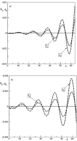
the period is T = 8. Numerical simulations have been performed with x = L/1280 andt = 1/2048. The relative error L1-norm on flow depth and discharge over a period has been found to vary in the range (0.9 ÷ 2)·10–4 for n = 0.4 and (0.9 ÷ 2)·10–5 for n = 1.5. Therefore, a more than satisfactorily agreement between numerical and analytical solutions has been observed. The exact and computed solutions are visually compared in terms of hp(x,t) and qp(x,t) for both the shear-thinning (Fig.
Fig. 1. Comparison between numerical (solid line) and analytical (symbols) solution: a) Shear-thinning fluid (n=0.4); b) Shear-thickening fluid
(n=1.5).
4. R
ESULTSIn the present section, the adoption of inlet boundary condition for the potential control of the spatial development of natural roll-waves in power-law fluids is investigated. To this aim, steep slope channels have to be considered and therefore the Froude number has to be chosen so that the uniform condition corresponds to both hypercritical and linearly unstable conditions: i.e. FN > FN,c and
FN > FN*. The effects of the upstream boundary
condition have been analyzed simulating the natural roll-waves development, through the numerical solution of the governing equations (Section 3), with different initial depth profiles. In the following, along with the uniform initial profile, both accelerated and decelerated hypercritical ones have been considered. As in the previous section, the power-law exponent n has been fixed to 0.4 (shear-thinning fluid) and 1.5 (shear-thickening fluid). The Froude number has been assumed equal to 3.0, for both cases. The following values of the critical flow depth hc = 2.15 (n = 0.4) and hc = 2.23 (n = 1.5) hold.
For both fluids, the accelerated and decelerated initial profiles have been evaluated by solving Eq. (12) through a second-order Runge-Kutta scheme, assigning different values of the flow depth at the channel inlet (hU). The hU value has been varied
between 0.5 and 0.9 hc, considering that Eq. (12) has
a singularity at h0 = hc. In what follows the values
hU= 0.5 and hU= 1.5 are preliminary considered,
along with the uniform case.
The dimensionless channel length is L = 640 and the adopted mesh spacing is x = 0.1. Fig. 2, in which for sake of clarity only a part of the channel has been shown, reports the calculated accelerated and decelerated initial profiles, along with the uniform one. As far as the shear-thinning fluid is concerned, Fig. 2a indicates that the uniform condition is essentially reached for both profiles in the first 30 channel length units, while this distance reduces to approximately one half in the shear-thickening case (Fig. 2b).
Fig. 2. Unperturbed uniform and gradually varying profiles: a) Shear-thinning fluid (n = 0.4); b) Shear- thickening fluid (n = 1.5).
Starting from initial unperturbed conditions, simulations have been carried out for a dimensionless duration of 4096. In the post-processing phase, the first 128 time units have been discarded to exclude the initial transient, in which the developing perturbation interests only part of the channel. Time-series of flow depth perturbation at selected locations were processed in order to compute basic statistics of the observed waves, that were detected based on the zero down-crossing method. The following statistical properties have been considered: the mean perturbation height at crests (h'max), the skewness parameter S = h'max/ h'min,
h'min being the mean height at the troughs, the mean
period of waves (T') and the mean asymmetry parameter (Babanin et al., 2007
)
N'
m m
m t t
N' A
1 2,
, 1
1 1
(25)
In Eq. (25) t1,m denotes the time interval between the
zero up-crossing and the wave peak of the m-th wave, t2,m the time interval between the peak and the zero
down-crossing time and N' the number of observed waves (N' > 100 in all simulations). The asymmetry and skewness parameters allow analyzing the non-linear waves evolution together with the breaking waves occurrence (Babanin et al., 2007). In particular, a wave with the front face steeper than the rear one implies a positive value of A while the limiting value A = 1 refers to the occurrence of downstream moving waves with shocks.
For the sake of clarity, the natural roll-waves development in uniform conditions is firstly discussed in the following subsection, while the case of the gradually varying unperturbed profiles is postponed to subsection 4.2
.
4.1
Natural Roll-waves Development in
Uniform Flow Condition
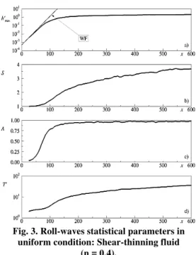
In Fig. 3, the profiles of the statistical properties, namely h'max (Fig. 3a), S (Fig. 3b), A (Fig. 3c) and T'
(Fig. 3d), are shown for the shear-thinning fluid. In Fig. 3a, for the sake of comparison, the exponential growth predicted by the linearized near wave-front analyses (WF), with the N growth rate given by
(A15), is also reported.
Downstream x ~ 10 and up to x ~ 60 the perturbations starts developing with a nearly exponential amplification (Fig. 3a), maintaining an almost skewness-free shape S ≈ 1, i.e. perturbations at peaks and troughs have the same mean magnitude (Fig. 3b). The roll-waves growth (Fig. 3a) is in good agreement with the theoretical results of the wave-front analyses. The A parameter is very small, indicating that the front and rear of the waves are approximately equally sloped (Fig. 3c). The mean wave period only slightly increases, confirming that the non-linear frequency reduction mechanism is paltry taking place (Fig. 3d). In conclusion, in this first part of channel, the non-linear effects are negligible and the main mechanism which governs the roll-waves spatial evolution is the instability of the base flow.
Fig. 3. Roll-waves statistical parameters in uniform condition: Shear-thinning fluid
(n = 0.4).
Downstream x ~ 60 and up to x ~ 200, the amplitude of the perturbation is so high that non-linear interactions among the waves take place. The waves begin to be non-symmetric (Fig. 3b), with the height at the crest larger than that at the trough. A decrease in the spatial growth-rate of peaks height is also observed (Fig. 3a). The wave period pronouncedly increases (Fig. 3d) suggesting that significant wave merging and coarsening processes are occurring. Finally, the asymmetry parameter rapidly increases reaching approximately a unitary value (Fig. 3c), enlightening that the front face of the waves is becoming always steeper than the rear one. Therefore, in this part of channel the non-linear interaction among the waves governs the spatial roll-waves evolution.
Downstream x ~ 200 a neat decrease in the growth-rate of crests is observed (Fig. 3a). The waves are characterized by an appreciable skewness (Fig. 3b), which increases in the downstream direction. Such a result is essentially associated to a constant value of the mean trough height h'min along the channel
processes are essentially independent of the perturbation magnitude, which however influences the spatial propagation along the channel, by shifting the abscissa at which the different evolution phases start to take place.
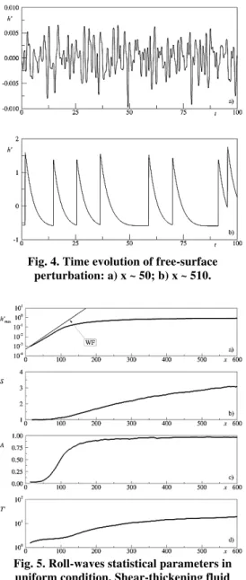
Fig. 4. Time evolution of free-surface perturbation: a) x ~ 50; b) x ~ 510.
Fig. 5. Roll-waves statistical parameters in uniform condition. Shear-thickening fluid
(n = 1.5).
Figure 5, which is the counterpart of Fig. 3 for the shear-thickening fluid, shows that the above described roll-waves evolution process, i.e. instability, merging, coarsening and breaking, is also found for the n = 1.5 case, therefore sharing strong similarities with the experimental evidence of Balmforth et al. (2005). In fact, the Authors, reproducing the roll-waves in cornstarch suspensions, observed that close to the chute inlet the waves were regular, and that they very quickly grew reaching relatively large amplitudes. In their evolution down the chute, a wave merging process was observed, ultimately leading to the coarsening of breaking waves.
The instability mechanism observed for both fluids
in the first part of the channel complies with the results achieved by Trowbridge (1987) on linearized depth-integrated momentum equations for both Newtonian and Bingham fluids. As far as the stability of uniform flow is concerned, Trowbridge (1987) showed that the multiplier to the velocity perturbation, arising from the linearized source term, plays a key role in defining the instability threshold. Such a term is essentially due to the increase of bottom stress produced by a velocity perturbation (u') and it reads
u u N
b
(26)
Indeed, according to Trowbridge (1987), flows with small values of the u' coefficient, i.e. b/u|N, are
more susceptible to be unstable. A similar conclusion was drawn by Di Cristo et al. (2009) in studying the instability of dense granular flows and by Coussot (1994) and Di Cristo et al. (2013a), as far as and Herschel & Bulkley fluid is concerned. For the present rheology, the u' coefficient is b/u|N = n,
and consistently FN* increases with n as predicted by
Eq. (24). Moreover, the comparison of Figs. 3 and 5 shows that for a constant value of FN, the
shear-thinning fluid, to which the smaller FN* is associated,
also exhibits a more pronounced spatial growth of the perturbations.
In the next subsection, the effect of a gradually varying profile on the pattern of roll-waves evolution from instability to breaking is addressed. As far as the initial stability phase is concerned, the Trowbridge conclusions, besides providing a physical explanation for uniform flow instability, will offer a simple and yet physically sound interpretation of the influence of the non-uniform profiles on the roll-waves spatial evolution (Section 4.2).
4.2 Natural
Roll-Waves
Development
in Gradually Varying Flow Conditions
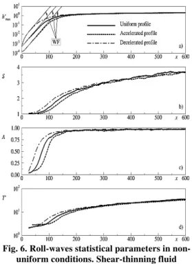
Fig. 6. Roll-waves statistical parameters in non-uniform conditions. Shear-thinning fluid
(n = 0.4).
Figures 6 and 7 show that also with decelerated/accelerated profiles the development of natural roll-wave trains follows the same general pattern outlined for the uniform flow case. Flow instability governs the perturbation growth in the upstream reach of the channel. Similarly to the uniform case, Fig. 6a and 7a show that close to the channel inlet the numerical results follow the theoretical findings of the wave-front analysis. Moving downstream, the waves progressively undergo merging and coarsening, increasing their amplitude but with a growth-rate reduction, and finally evolve into trains of breaking waves. However, relevant differences appear in the response to non-uniform inlet condition for both shear-thinning and shear-thickening fluids.
As far as the shear-thinning case is concerned, the effect of the boundary condition on the instability-dominated phase is evident. The accelerated initial profile slows down the growth of peaks, while the opposite behavior is observed for the decelerated one (Fig. 6a). Both skewness and asymmetry parameters (Figs. 6b,c) confirm such a conclusion and moreover, the minor growth of the wave period close to the channel inlet is also coherent with the stabilizing effect of the accelerated profile.
The stabilizing (resp. destabilizing) effect of the accelerated (resp. decelerated) profile may easily explained looking at the linearized version of the momentum equation, i.e. the second equation of system (7):
h F x u u
x h F h u t
u
b N
N
1 1 1
2
1 1
2 2 2
(27)
By perturbing the initial condition in Eq. (27), i.e.
setting u(x,t) = u0(x)+u'(x,t) and h(x,t) = h0(x)+h'(x,t) with u' << u0 and h' << h0, and by accounting for Eq. (12) the following linearized momentum equation can be easily deduced :
hh u h
h h F
u u F h x u
x u u x
h F t u
b b N
b N N
2 0 2 0 2
0 0 0 2
0 2 0 0
0 2
1 1
1
1 d d
1 2 1
(28)
Equation (28) suggests that a spatial velocity variation in the initial condition, i.e. du0/dx generates an additional term proportional to u'. Accounting for the positivity of b/u|0(Eq. (5)), such an additional
term increases (resp. reduces) the magnitude of the u' coefficient in Eq. (28) in presence of accelerated (resp. decelerated) profiles. Therefore, accordingly with Trowbridge (1987) findings, the spatial variation of the velocity in the initial condition appears to be one of the main reasons for the increased (resp. reduced) stability of the accelerated (resp. decelerated) initial profiles.
The different growth of the disturbance close to the channel inlet induces a shift downstream (resp. upstream) for the accelerated (resp. decelerated) profile of the location where the non-linear effects begin to be relevant, and therefore of the abscissa where the coarsening process starts to take place. Indeed, the change in the trend of the T' distribution is seen to occur, with respect to the uniform condition, upstream (resp. downstream) in the decelerated (resp. accelerated) condition (Fig. 6d). Figures 6b and 6c lead to a similar conclusion for both the S and A parameters.
Starting from the channel abscissa at which the coarsening process begins, its successive evolution appears to be independent of the initial profile, as deduced also from Figs. 6b,c,d. Such a result may be explained considering that, independently of the initial profiles, in the channel section at which the coarsening process starts to take place the uniform condition has been recovered (Fig. 2a). Therefore, the coarsening process occurs with the same dynamics for all profiles, maintaining the shift occurred the initial phase. As a matter of fact, the distance from the channel inlet at which permanent waves with shocks occur, i.e. where A ≈ 1, is more downstream (resp. upstream) in the accelerated (resp. decelerated) case than in presence of uniform profile (Fig. 7c).
the effect of the decelerated profile is more magnified in the case of the shear-thickening fluid than in the shear-thinning one. This is consistent with the behavior of the 1 and 2 coefficients (see Fig. A1), which have larger values in the n = 1.5 case for h0 < 1. As described in the Appendix in the framework of the linear assumption, these two coefficients play a key role on the growth/decay of an initial perturbation. For small values of the flow depth, while their values remain bounded for shear-thinning fluids, for shear-thickening ones they positively diverge.
Fig. 7. Roll-waves statistical parameters in non-uniform conditions. Shear-thickening fluid
(n = 1.5).
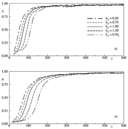
To further enlighten the effect of the initial profile on the roll-waves development, Fig. 8 depicts the profiles along the channel of the mean asymmetry parameter for different investigated inlet boundary conditions, for both the shear-thinning (Fig. 8a) and the shear-thickening (Fig. 8b) fluids. Figure 8 clearly indicates that an increase of the hU value induces a
progressive monotone downstream shift of the portion of the channel where non-linearity onsets. This results is coherent with the monotonically decreasing behavior of the 1 and 2 coefficients (Fig.A1) observed both thinning and shear-thickening fluids for h0 > 0.5. Moreover, results of Fig. 8 confirms that, independently of the inlet boundary condition, the growth rate in the non-linear interaction phase is profile independent.
Based on the above results, it appears possible, in steep slope channels, to alter the roll-waves development by prescribing an appropriate inlet boundary condition. Further theoretical analyses, with more sophisticated models than the von Kármán one, and experimental validations could provide a more detailed picture of the investigated phenomenon. However, the above findings clearly indicate that, for a given channel length, an inlet condition determining an accelerated (resp. decelerated) profile may be used to suppress (resp.
promote) the final stage of the roll-waves development. Such a conclusion therefore supports a potential strategy for the passive control of roll-waves in power-law fluids.
Fig. 8. Spatial distribution of mean asymmetry parameter for different values of the inlet boundary condition: a) Shear-thinning (n = 0.4);
b) Shear-thickening (n = 1.5).
5. C
ONCLUSIONSIn the present paper the potentiality of the inlet control of natural roll-waves development in hypercritical films of power-law fluid has been exploited. Both thinning and shear-thickening fluids have been considered. Owing to the hypercritical character of the base flow, the flow depth assigned at the inlet dictates, for a given discharge, the gradually-varying profile which may strongly differ from the uniform one. Initial accelerated, decelerated and uniform profiles have been investigated. The analysis has been carried out by numerically solving the von Kármán depth- integrated mass and momentum conservation equations, in the long-wave approximation, through a second-order finite volume scheme. For a given initial profile, the roll-waves have been generated perturbing the flow rate at the inlet with a small random white-noise and the spatial evolution of the perturbations has been analyzed. For both clear-water and granular flows, such a technique has been shown to be able to describe the main features of the natural roll-waves. The spatial evolution along the channel of the roll-waves has been represented evaluating the mean perturbation height at the crests, the wave mean period, the skewness and the asymmetry parameters. Under the same perturbation the effect of the inlet boundary condition on the roll-waves spatial evolution has been analyzed.
growth-rates of the natural roll-waves comply with the theoretical ones coming from the linear analysis. Such a result confirms the validity of the linearized model to describe the roll-waves spatial growth in the first phase of their formation.
The main conclusion of the present study is that roll-waves spatial evolution is strongly affected by the initial profile, suggesting the possibility of a their passive control through inlet operations. Independently on the rheological parameter, a decelerated initial profile promotes the instability mechanism, whereas an accelerated one demotes it. This effect induces a shift, either upward or downward, of the abscissa where the non-linear waves interaction starts to take place. However, once the coarsening dynamics begins, it evolves in a similar way independently of the initial profile. Therefore, the aforementioned shift affects also the abscissa at which the final phase of the roll-waves development starts.
In conclusion, the present results show that through a suitable boundary condition, it would be possible for a given channel length to inhibit or promote the roll-waves development. Therefore, inlet control may be an effective and promising strategy for the passive control of natural roll-waves development. Useful additional details on this aspect may be furnished by further theoretical/numerical analyses with more complex model and/or experimental tests.
6. A
PPENDIXThe present Appendix describes some details about the near wave-front expansion analysis applied for studying the stability of a gradually varying profile. Present developments extend the stability analysis of Campomaggiore et al. (2016a) to the case of a discontinuity on spatial derivatives of order larger than one. The technique considers that for any hyperbolic system a discontinuity of the unknown derivatives propagates in the (x,t) plane along the characteristic line with slope0. The spatial evolution of a discontinuity on each derivative at x=0 may be analyzed, developing the unknown functions in Taylor expansion, close to the wave-front. Introducing the following variable transformation
,
x
d0dtdx (A1)
the governing equations (Eq. (7)) in the new reference are:
u u u s
u A u 0 (A2)
Following the procedure developed in Campomaggiore et al. (2016a), the unknown vector, the matrix A and the source terms are expanded in powers of around = 0, whose substitution in (A2) leads tothe following system:
... ! 3 ! 2 ... 2 ... ! 3 ! 2 ... ! 3 ! 2 ... ! 3 ! 2 ... 2 3 3 2 2 1 0 2 3 2 1 3 3 2 2 1 0 3 3 2 2 1 0 3 3 2 2 1 0 2 3 2 1 0 s s s s u u u A A A A u u u u A A A A u u u (A3)
in which for sake of clarity the explicit dependence has been omitted. Denoting with I the identity matrix and accounting for Eq. (12), at different powers of
, Eq. (A3) generates the following systems: zero order:
0IA0
u10 (A4) first order:
0 0
2 0 1 1 0 1 1 1d d d d s u A u A u A u A
I
(A5) second order:
2 1 2 2 1 0 2 1 1 2 0 3 0 0 2 d d d d 2 d d s u A u A u A u A u A u A I (A6) third order:
3 1 3 2 2 3 1 0 3 1 2 2 1 3 0 4 0 0 3 3 d d d d 3 d d 3 d d s u A u A u A u A u A u A u A u A I (A7)Owing to the 0 and l0 definitions, the matrix
0IA0
is rank-deficient and moreover
0 0
1 00
i T u A I
l
, for all ui+1 vectors.Therefore, once the ui-1 function is known, the
system of equations for each ui may be easily
deduced. In detail, the spatial evolution of u1 is described by Eq. (A4) and the following equation:
0 d d d d 1 1 1 0 1 0 1 0
0
u Au s
A l u l
T T
(A8)
2
0 d d d d 2 d d 2 1 2 2 1 0 0 2 1 1 0 2 0 0 s u A u A l u A u A l u l T T T (A9)Similarly, the governing equations for u3 are Eq. (A6) together with:
3
03 d d d d 3 d d 3 d d 3 1 3 2 2 0 3 1 0 3 0 1 2 2 1 0 3 0 0 s u A u A l u A u A l u A u A l u l T T T T (A10)
Of course, approximations at order larger than the third one may be easily found in a similar way. The stability of a gradually varying profile of a power-law fluid, at the first-order of approximation has been carried out in Campomaggiore et al. (2016a). In what follows only the major results will be reported. Eqs. (A4) and (A8) may be combined to deduce the following differential equation involving only the h1() function:
0d d 1 1 2 1 1
1 h h
h
(A11) in which
I II f f 1
I III f f 1 (A12) where:
0 0
20 0
2 h
h
fI (A13a)
20 4 0 2 3 0 2 0 0 0 2 3 2 2 2 N II F h h h h
f
(A13b)
2 2 0 2 0 0 0 2 0 3 0 2 0 0 0 0 2 1 2 d d 6 1 8 2 1 n N N N III h F h n h h h F h h F f (A13c)For small h1 values the non-linear term in Eq. (A11) may be neglected and its solution is (Campomaggiore et al., 2016a):
0 1 d1 e (A14)
which enlightens the key role of the 1 coefficient on the growth or the decay of an initial perturbation, within the linear assumption. In particular, whenever the 1 coefficient is positive (resp. negative) the disturbance grows (resp. decays) along the entire channel, and therefore flow is unstable (resp. stable). In uniform conditions, the 1 coefficient is a constant
and it reads:
21 2 N N N N N F n (A15)
Eqs. (A14) and (A15) suggests that an exponential growth (resp. decay) is expected in linear unstable (resp. stable) conditions of flow. A detailed discussion concerning the effects on the linear stability of initially gradually profiles for both shear-thinning and shear-thickening power-law fluids may be found in Campomaggiore et al. (2016a). The same paper discusses also the role of the non-linear term appearing in Eq. (A11), which is responsible of non-linear wave breaking, i.e. the divergence of h1 at a finite abscissa.
The stability of the base flow to a discontinuity only in the second spatial derivative (an abrupt change in free-surface curvature) may be investigated based on Eqs. (A5) and (A9) assuming u1 = 0. Such an analysis has provided useful insights in studying the propagation of wave front in viscoelastic arteries (Holenstein et al., 1984) and it may offer useful information in studying the natural roll-wave formation, where a random disturbance is imposed. Indeed, using Eq. (A5), it easy to verify that the following relation holds:
0 2 0 0 2 0 22 1 1
1 h h u F h u F F
u N N
N
(A16)
Accounting for Eq. (A16) in Eq. (A9), along with the expressions of A2 and s2:
2 3 0 2 0 2 0 0 0 2 1 2 0 1 1 2 0 0 2 1 3 0 2 0 2 22 2 1
2 2 2 2 1 u h h u u h h u u h h u h u h h u h u A (A17)
2 1 1 0 2 0 2 2 0 0 2 0 2 0 2 0 1 0 2 1 3 0 0 2 1 1 2 0 1 0 2 2 2 1 2 3 2 0 2 1 u h u n n h h u u h h u h u n h h u n n h u h u n n F n n n n n n n n n n N s (A18) the following equation for the h2() function isdeduced:
0d d
2 2
2 h
h
(A19)
in which:
I III f fˆ2
(A20)
where
0 0
0 u
c (A22)
Differently from the first order case, Eq. (A19) is linear in h2 and therefore the discontinuity on the second-order spatial derivative cannot lead to a breaking wave.
If a linear approximation (h1 → 0) is assumed in Eq. (A11), a comparison between the development of discontinuities of first and second derivatives analysis may be easily carried out comparing the 1 and 2 coefficients. In uniform flow conditions (i.e. h0=1 and dh0/d = 0) 2 = 1 (Eqs. (A20)-(A21)), therefore the results pertaining to the first derivative discontinuity (Campomaggiore et al., 2016a) apply also to the second order one. In particular, stable conditions are characterized by Froude number values smaller than *
N
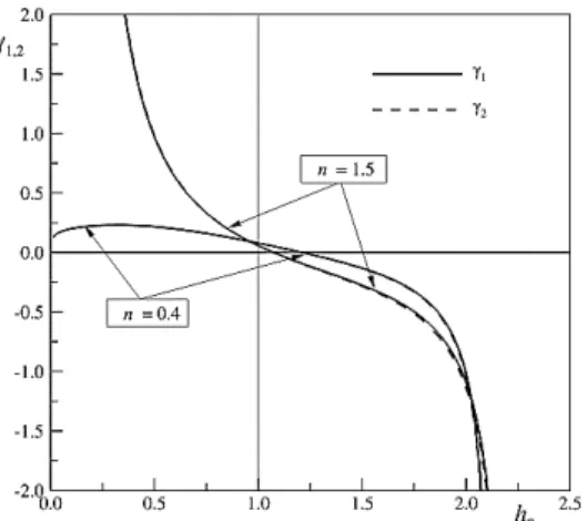
F
given by Eq. (24).In order to enlighten the differences between the results of the first and the second order analyses, Fig. A1 compares the and coefficients dependence on the flow depth h0 for the shear-thinning (n = 0.4) and the shear-thickening (n = 1.5) fluids. The same flow condition of the previous sections, i.e. FN = 3.0,
is considered.
Fig. A1. Growth rate coefficients as function of the flow depth.
Figure A1 indicates that, for flow depths smaller than the uniform value (h0<1), the and coefficients essentially coincide, while only small differences are visible for h0> 1. Even for a perturbation on the second derivative, although the uniform hypercritical condition is linearly unstable, the disturbance growth is inhibited by an accelerated profile, while it is promoted by a decelerated one. In the latter flow condition, the effect is magnified for shear-thickening fluids, for which a divergence of the growth rate occurs for vanishing flow depth. Such a difference may be explained accounting for the different behavior of the free surface slope for
h0 → 0. Indeed, Eq. (12) shows that for h0 → 0, while
shear-thinning fluids are characterized by dh0/dx → 0, for the shear-thickening fluids the free-surface slope diverges inducing an unbounded growth of both and coefficients, and in turn of
the perturbation. Conversely, independently of the fluid rheology, for h0 → hc (hc = 2.15 shear-thinning
case; hc = 2.23 shear-thickening case) the
free-surface slope diverges (see Eq. (12)) and therefore the negative values of both and coefficients are unbounded.
A
CKNOWLEDGMENTSPart of this research has been supported by both Regione Campania [grant LR5/02-2008 no. B36D14000770002] and Chilean Science and Technology Fund [grants Fondecyt no. 11309910 and 1161751].
R
EFERENCESBabanin, A., D. Chalikov, I. Young, and I. Savelyev (2007). Predicting the breaking onset of surface water waves. Geophysical Research Letters, 34(7).
Balmforth, N. J., I. A. Frigaard and G. Ovarlez (2014). Yielding to stress: recent developments in viscoplastic fluid mechanics. Annual Reviews of Fluid Mechanics 46, 121-146.
Balmforth, N. J., J. W. M. Bush and R. V. Craster (2005). Roll waves on flowing cornstarch suspension. Physics Letter A 338, 479-484. Bohorquez, P. and M. Rentschler (2011).
Hydrodynamic instabilities in well-balanced finite volume schemes for frictional shallow water equations. The kinematic wave case. Journal of Scientific Computing 48(1-3), 3-15.
Bouchut, F. and S. Boyaval (2013). A new model for shallow viscoelastic fluids. Mathematical Models and Methods in Applied Sciences 23, 1479-1526.
Bouchut, F. and S. Boyaval (2014). Unified formal reduction for fluid models of free surface shallow gravity-flows. arXiv, 1306.3464. Brock, R. (1967). Development of roll waves in open
channels. W.M. Keck Lab. of Hydraul. and Water Resources, California, Inst. of Tech. Report KH-R-16, 226.
Campomaggiore, F., C. Di Cristo, M. Iervolino and A. Vacca (2016a). Development of roll waves in power-law fluids with non-uniform initial conditions. Journal of Hydraulic Research 54(3), 289-306.
Campomaggiore, F., C. Di Cristo, M. Iervolino and A. Vacca (2016b). Inlet effects on roll-waves development in shallow turbulent open-channel flows. Journal of Hydrology and Hydromechanics 64(1), 45-55.
Cao, Z., P. Hu, K. Hu, G. Pender and Q. Liug (2015). Modelling roll waves with shallow water equations and turbulent closure. Journal of Hydraulic Research 53(2), 161-177.
solutions. The Canadian Journal of Chemical Engineering 57, 135-140.
Chang, H. C., E. A. Demekhin and E. Kalaidin (2000). Coherent structures, self-similarity, and universal roll wave coarsening dynamics. Physics of Fluids 12, 2268-2278.
Coussot, P. (1994). Steady, laminar, flow of concentrated mud suspensions in open channel, Journal of Hydraulic Research 32(4), 535-559.
Craster, R. V. and O. K. Matar (2009). Dynamics and stability of thin liquid films. Reviews of Modern Physics 81(4), 1131-1198.
Di Cristo, C., M. Iervolino and A. Vacca (2013a). Waves Dynamics in a Linearized Mud-Flow Shallow Model. Applied Mathematical Sciences 7(83), 377-293.
Di Cristo, C., M. Iervolino and A. Vacca (2013b). Gravity-Driven Flow of a Shear-Thinning Power–Law Fluid over a Permeable Plane. Applied Mathematical Sciences 7(33), 1623-1641.
Di Cristo, C., M. Iervolino and A. Vacca (2015). On the stability of gradually varying mudflows in open channels. Meccanica 50(4), 963-979. Di Cristo, C., M. Iervolino, A. Vacca and B.
Zanuttigh (2009). Roll waves prediction in dense granular flows. Journal of Hydrology 377(1-2), 50-58.
Edwards, A. N. and J. M. N. T. Gray (2015). Erosion-deposition waves in shallow granular free-surface flows. Journal of Fluid Mechanics 762, 35-67.
Fernandez-Nieto, E. D., P. Noble and J. P. Vila (2010). Shallow water equations for non-Newtonian fluids. Journal of Non-non-Newtonian Fluid Mechanics 165, 712-732.
Gottlieb, S. and C. W. Shu (1998). Total variation diminishing Runge–Kutta schemes. Mathematics of Computations 67(221), 73-85.
Harten, A. (1983). High resolution schemes for hyperbolic conservation laws. Journal of Computational Physics 49, 357-393.
Heining, C. and N. Aksel (2010). Effects of inertia and surface tension on a power-law fluid flowing down a wavy incline. International Journal of Multiphase Flow 36(11–12), 847-857.
Holenstein, R., R. M. Nerem and P. F. Niederer (1984). On the Propagation of a Wave Front in Viscoelastic Arteries. Journal of Biomechanical Engineering 106, 115-122.
Huang, Z. and J. J. Lee (2015a). Modeling the spatial evolution of roll waves with diffusive saint venant equations. Journal of Hydraulic
Engineering 141(2).
Huang, Z., and J. J. Lee (2015b). Numerical investigation on roll-waves proprieties: wave-wave interactions, generality and spectrum. Journal of Engineering Mechanics 141(2).
Miladinova, S., G. Lebon, and E. Toshev (2004). Thin-film flow of a power–law liquid falling down an inclined plate. Journal of Non-Newtonian Fluid Mechanics 122, 69-78.
Ng, C. and C. C. Mei (1994). Roll waves on a shallow layer of mud modeled as a power-law fluid. Journal of Fluid Mechanics 263, 151-184. Pascal, J. P. (1999). Linear stability of fluid flow
down a porous inclined plane. Journal of Physics D 32, 417-422.
Pascal, J. P. (2006). Instability of power-law fluid flow down a porous incline. Journal of Non-Newtonian Fluid Mechanics 133, 109-120.
Roe, P. L. (1986). Discrete models for the numerical analysis of time-dependent multidimensional gas-dynamics. Journal of Computational Physics 63, 458-476.
Sadiq, I. M. R. and R. Usha (2008). Thin Newtonian film flow down a porous inclined plane: Stability analysis. Physic of Fluids 20(2). Sadiq, I. M. R. and R. Usha (2010). Effect of
permeability on the instability of a non-Newtonian film down a porous inclined plane. Journal of Non-Newtonian Fluid Mechanics 165, 1171-1188.
Supino, G. (1960). On surge waves in channels. Report of the Lincei National Academy 295(6), 543-552
Trowbridge, J. H. (1987). Instability of concentrated free surface flow. Journal of Geophysical Research 92, 9523-9530.
Usha, R., S. Millet, H. Ben Hadid and F. Rousset (2011). Shear-thinning film on a porous substrate: Stability analysis of a one-sided model. Chemical Engineering Science 66(22), 5614-5627.
Witham, G. B. (1974). Linear and nonlinear waves. John Wiley and Sons Interscience, New York. Yadav, A., S. Chakraborty and R. Usha (2015).
Steady solution of an inverse problem in gravity-driven shear-thinning film flow: reconstruction of an uneven bottom substrate. Journal of Non-Newtonian Fluid Mechanics 219, 65-77..