Thiago Antonini Alves
Member, ABCM [email protected]Carlos A. C. Altemani
Emeritus Member, ABCM[email protected] Universidade Estadual de Campinas – UNICAMP Faculdade de Engenharia Mecânica Departamento de Energia 13083-970 Campinas, SP, Brazil
Convective Cooling of Three Discrete
Heat Sources in Channel Flow
A numerical investigation was performed to evaluate distinct convective heat transfer coefficients for three discrete strip heat sources flush mounted to a wall of a parallel plates channel. Uniform heat flux was considered along each heat source, but the remaining channel surfaces were assumed adiabatic. A laminar airflow with constant properties was forced into the channel considering either developed flow or a uniform velocity at the channel entrance. The conservation equations were solved using the finite volumes method together with the SIMPLE algorithm. The convective coefficients were evaluated considering three possibilities for the reference temperature. The first was the fluid entrance temperature into the channel, the second was the flow mixed mean temperature just upstream any heat source, and the third option employed the adiabatic wall temperature concept. It is shown that the last alternative gives rise to an invariant descriptor, the adiabatic heat transfer coefficient, which depends solely on the flow and the geometry. This is very convenient for the thermal analysis of electronic equipment, where the components’ heating is discrete and can be highly non-uniform.
Keywords: adiabatic heat transfer coefficient, laminar channel flow, discrete heat sources, numerical investigation, electronics cooling
Introduction
1
The convective heat transfer from an isothermal surface to a fluid flow is expressed through a simple definition of a heat transfer coefficient, as indicated in Eq. (1).
(
)
r w r
q=h A T −T (1)
In this equation, q indicates the convective heat transfer rate and A represents the heat transfer area. Tw is the isothermal surface temperature and Tr is a fluid reference temperature. The choice of the reference temperature Tr in Eq. (1) defines the corresponding convective heat transfer coefficient hr.
For uniform thermal boundary conditions, the reference temperature Trmay be conveniently chosen. In external flows, for example, it is equal to T∞, the fluid free stream temperature far from the heat transfer surface, and the corresponding convective coefficient is h∞. In internal flows, the reference is usually the local mixed mean fluid temperature Tm and the corresponding heat transfer coefficient is hm, but sometimes the fluid inlet temperature Tin is also chosen as the reference, giving rise to hin. Uniform boundary conditions and these reference temperatures usually lead to either a uniform or a monotonically varying convective heat transfer coefficient along the heat transfer surface.
There are however practical situations with non-uniform thermal boundary conditions in the flow direction. In these cases, the standard reference temperatures, like T∞ in external flows and either Tm or Tin in internal flows, may lead to a very strange behavior of the corresponding heat transfer coefficient. A discontinuity in the wall temperature distribution, for example, may lead to a discontinuity of the local heat transfer coefficient from –∞ to +∞ (Kays and Crawford, 1993).
In electronics cooling, a typical circuit board may contain several discrete components, all dissipating electric power at distinct rates on their surfaces. The standard convective heat transfer coefficients based either on T∞, Tm, or Tin may pose two main difficulties in this case. First, a step change on the board wall temperature from one component to the next may cause a discontinuity in the heat transfer coefficient from –∞ to +∞ along the board. Second, the electric power dissipation in the components
Paper accepted April, 2008. Technical Editor: Demétrio Bastos Neto.
could change, leading to distinct distributions of the heat transfer coefficient for each case. Worse, the values of these coefficients for any set of thermal boundary conditions on the circuit board would not be useful to the analysis of any additional proposed change.
These difficulties can be avoided if Tr in Eq. (1) is associated to the adiabatic surface temperature Tad of any component on the circuit board. This is the temperature the component attains when its power dissipation rate is turned to zero while all the other components are dissipating power at their specified rates. If Tad is used as the reference temperature in Eq. (1), the adiabatic heat transfer coefficient had is obtained. This concept was introduced by Arzivu and Moffat (1982) from experiments in electronics cooling and extended by subsequent works of Arzivu et al. (1985), Anderson and Moffat (1992a, 1992b), Moffat (1998) and Moffat (2004). They showed that the adiabatic heat transfer coefficient is an invariant descriptor of the convective heat transfer. It is independent of the thermal boundary conditions, being a function only of the geometry and flow characteristics – a brief description, based on these works, will be presented.
parallel-plates channel. They defined the convective heat transfer coefficient using the channel flow inlet temperature as the reference in Eq. (1). Ortega and Lall (1992) considered a small strip heat source (qs′′) flush mounted to one wall of a parallel-plates channel. The wall thermal boundary condition was either adiabatic (qw′′ = 0) or a uniform heat flux (qw′′ < qs′′) downstream and upstream the heat source. They investigated numerically the effect of the heat source position along the channel length on the average Nusselt number over the heat source. The analysis was performed under conditions of laminar developing flow and also fully developed flow at the channel entrance. The Nusselt number was defined using the local mixed mean temperature (Tm) and also the adiabatic temperature (Tad) as the reference. For fully developed flow at the channel entrance, the average Num over the heat source was independent of the heat source position when the upstream wall was adiabatic. When the upstream wall was heated, the source average Num decreased along the channel length. On the other hand, for the same flow and thermal conditions, the heat source average value of Nuad was uniform along the channel length, independently of the upstream wall thermal conditions. Moffat (1998) presented the quest for invariant descriptors of the convective process which can deal with non-uniform thermal boundary conditions. He presented a historical review of the heat transfer coefficient, with emphasis on had and Tad and described some difficulties in measuring these quantities. Experimental results for the heat transfer coefficient on heated blocks in a channel were presented and it was shown that the related measurements of Tad should be made very accurately else the derived coefficients would be useless.
In the present work, three distinct heat transfer coefficients, defined for the reference temperatures Tin, Tm and Tad, were obtained from numerical simulations for the configuration indicated in Fig. 1. Three strip heaters flush mounted to a wall of a parallel plates channel were cooled by a forced air flow in the laminar regime. The properties needed for calculating the flow and heat transfer parameters of this problem were evaluated at the film temperature, as recommended in the literature (Bejan, 1995). Two distinct flow conditions at the channel inlet were investigated – a developed flow and a developing flow starting with a uniform velocity profile. Each heater had the same length Lh and the spacing from one heater to another was Ls. Their position in the channel was defined by the upstream length Lu and the downstream length Ld. The channel height was Lc, as indicated in Fig.1, and the simulations were performed for the conditions Lu = 5 Lc, Ld = 10 Lc and considering Lh = Ls = Lc. From these relations, the total channel length was L = 20 Lc.
Figure 1. Parallel plates channel with three flush mounted heaters.
Nomenclature
A = heat transfer area, m2 cp = specific heat, J/kgK g* = influence coefficient
h = convective heat transfer coefficient, W/m2 K k = thermal conductivity, W/mK
L = total channel length, m
Lc = channel height, m Ld = downstream length, m Lh = heater length, m
Ls = spacing between heaters, m Lu = upstream length, m
m& = mass flow rate, kg/s Nu = Nusselt number,Eq. (19) P = pressure, Pa
P* = dimensionless pressure, Eq. (15) Pr = Prandtl number
q = convective heat transfer rate, W q′′ = heat flux, W/m2
Re = Reynolds number, Eq. (10) T = temperature, K
u = velocity component along the plates, m/s U = dimensionless u – velocity component, Eq. (15) v = velocity component normal to the plates, m/s V = dimensionless v – velocity component, Eq. (15) x, y = Cartesian coordinates, m
X, Y = dimensionless Cartesian coordinates, Eq. (15)
Greek Symbols
ρ = density, kg/m3
µ = dynamic viscosity, Pa/s
θ = dimensionless temperature, Eq. (15) υ = kinematic viscosity, m2/s
Subscripts
ad adiabatic
i ith heater of the array in inlet
m mixed mean n nth heater of the array r reference
s strip heat source
w wall
∞ free stream Superscripts – average
Analysis
The adiabatic heat transfer coefficient
Consider a two-dimensional array of heaters flush mounted to a channel wall, such as that indicated in Fig. 1. The adiabatic heat transfer coefficient for the nth heater of the array is most easily obtained assuming it is the single active heater while all the others are kept inactive. Under these conditions, the adiabatic surface temperature of the active heater is the fluid temperature at the channel inlet (Tad = Tin). Then, the active heater temperature rise above its adiabatic temperature (Tw –Tad) is due solely to self-heating and Eq. (1) defines the corresponding adiabatic heat transfer coefficient. The convective heat rate qn released by the nth heater causes a mixed mean temperature rise (∆Tm)n related to the mass flow rate in the channel by an energy balance.
(
)
nm n p q T
m c
∆ =
& (2)
Applying a procedure similar to that of Anderson and Moffat (1992b) to the considered two-dimensional array, the temperature differences (Tw – Tad)n and (∆Tm)n were related by the definition of an influence coefficient g*(n–n).
#1
x
Lu
L
m&
#2 #3
Lh Ls Ld
(
) (
) (
*)
n *(
)
w ad n m n
p q
T T T g n n g n n
m c
− = − = −
&
∆ (3)
When two or more heaters are simultaneously active, the temperature rise of any heater is due to both the self-heating and the thermal wake effect from the upstream active heaters. The thermal wake increases the adiabatic temperature of all downstream heaters above the inlet fluid temperature Tin. These two effects can be expressed by
(
Tw−Tin) (
n= Tw−Tad) (
n+ Tad−Tin)
n (4)If the fluid flow were perfectly mixed, (Tad –Tin)n would be equal to the mixed mean temperature rise due to all upstream active heaters. Due to imperfect mixing however, (Tad –Tin)n will always be higher than this mixed mean temperature rise. The contribution of an active heater in the ith row of the array to the adiabatic temperature rise of a downstream heater in the nth row can be described by the definition of an influence coefficient g*(n-i) defined by
(
)
(
) (
)
i(
)
ad in n i m i
p q
T T T g n i g n i
m c
∗ ∗
−
− = − = −
&
∆ (5)
Taking into account the effects of all the active heaters upstream the nth row of the two-dimensional array, the definitions of the two influence coefficients can be replaced into Eq.(4) resulting in
(
)
n(
)
i(
)
w in n
i
p p
q q
T T g n n g n i
m c m c
∗ ∗
− = − +
∑
−& & (6)
From Equations (3) and (6), expressions for had and hin can be obtained as follows.
(
n)
(
p)
ad ,n
w ad n n mc q
h
T T A g∗ n n
′′
= =
− −
&
(7)
(
n)
(
)
n(
)
in ,n
n i
w in n
i
p p
q q
h
q q
T T g n n g n i
m c m c
∗ ∗ ′′ ′′ = = − − +
∑
− & & (8)As indicated by Moffat (1998), there are no thermal boundary conditions in Eq. (7), i.e., had is a function of flow parameters only. For the same geometry and flow conditions, the value of had obtained by any type of test will be the same for any other thermal conditions. Considering a convective cooled circuit board populated with several heaters, the value of had for any heater will not depend on the distribution of electric power dissipation. Comparatively, the correlation for hin is much more complex, involving the heat flow from each upstream heater on the board. In Equation (8), the value of hin will be the same for any level of heating only when all the heaters dissipate heat at the same rate.
Problem Formulation and Heat Transfer Parameters
The flow in the channel depicted in Fig. 1 was considered in the laminar regime under steady state conditions and constant fluid properties. The velocity and temperature profiles were obtained by numerical simulations using the control volumes method (Patankar, 1980) and the SIMPLE (Semi-Implicit Method for Pressure Linked Equations) algorithm. At the channel entrance, the flow was assumed either developed or with a uniform velocity profile.
When the flow was assumed developed from the channel entrance, the parabolic profile of the analytical solution was assumed and the numerical simulations were performed only for the temperature distribution in the channel. In this case, the velocity component normal to the plates (v) was zero and that along the plates (u) was
( )
22
3 4
1
2 c
y
u y u
L
⎛ ⎞
= ⎜⎜ − ⎟⎟
⎝ ⎠ (9)
A Reynolds number was defined, using the channel hydraulic diameter, as
2
h c
u D u L
Re= =
υ υ (10)
Five values of Re were employed in the numerical simulations: 630, 945, 1260, 1575 and 1890. For Lc = 0.01 m and considering that the fluid is air at 300 K, these five values correspond to average velocities along the channel respectively close to 0.50 m/s, 0.75 m/s, 1.00 m/s, 1.25 m/s and 1.50 m/s. Under these conditions, axial conduction in the fluid is negligible relative to transversal conduction (Kays and Crawford, 1993).
When the velocity profile was considered uniform at the channel entrance, the simultaneous development of the velocity and temperature profiles were obtained from the numerical solution of the conservation equations of mass, momentum and energy. These equations were expressed in dimensionless form as follows.
0
U V
X Y
∂ +∂ =
∂ ∂ (11)
2 2
2 2
U U P U U
U V
X Y X X Y
∗
∂ + ∂ = −∂ +⎛∂ +∂ ⎞
⎜ ⎟
∂ ∂ ∂ ⎝∂ ∂ ⎠ (12)
2 2
2 2
V V P V V
U V
X Y Y X Y
∗
∂ + ∂ = −∂ +⎛∂ +∂ ⎞
⎜ ⎟
∂ ∂ ∂ ⎝∂ ∂ ⎠ (13)
2
2 1
U V
X Y Pr Y
∂θ+ ∂θ= ⎛∂ θ⎞
⎜ ⎟
∂ ∂ ⎝∂ ⎠ (14)
The dimensionless variables used in the conservation equations were defined by
x X
L = , Y y
L
= , U=ρu L
µ ,
v L
V=ρ
µ ,
2
2 P L
P∗= ρ
µ , in s h T T q L k − θ = ′′
⎛ ⎞
⎜ ⎟
⎝ ⎠
(15)
The boundary conditions for the developing flow encompassed a uniform velocity at the channel entrance and no-slip at the channel walls. The thermal boundary conditions were a uniform temperature at the channel inlet, equal to Tin, and an adiabatic condition at the channel walls, except along any active heater, where a uniform heat flux was considered.
surface temperature and the chosen reference temperature Tr (either Tin, Tm, or Tad).
n r ,n
h ,n r ,n q h
T T
′′ =
− where
( )
1
h
h ,n h ,n h L
T T x dx
L
=
∫
(16)When Tin was chosen as the reference temperature, it is evident from Eq. (15) that θin,n = 0. If the selected reference was the mixed mean Tm, it was evaluated numerically at the upstream end of the considered active heater. For constant fluid properties, it was obtained from
c
c
A m ,n
A uTdA
T
udA =
∫
∫
and m ,n m ,n in s hT T
q L k
−
θ = ′′
⎛ ⎞
⎜ ⎟
⎝ ⎠
(17)
For the choice of the adiabatic wall temperature Tad as the reference, its value was obtained from the average heater surface temperature when its power was turned off and there were other active upstream heaters.
( )
1h
ad ,n ad ,n h L
T T x dx
L
=
∫
and ad ,n inad ,n
s h
T T
q L k
θ = ′′−
⎛ ⎞
⎜ ⎟
⎝ ⎠
(18)
The heater length Lh was chosen the characteristic length for the average Nusselt number due to the thermal boundary layer nature of the heat transfer from the strip heaters. Using the heat transfer coefficient defined by Eq. (16), the average Nu for the nth heater of the array was
1 r ,n h r ,n
w,n r ,n h L
Nu k
= =
θ − θ (19)
Considering a single active heater in the channel, the fluid mixed mean temperature upstream the heater and its adiabatic surface temperature are equal to the fluid inlet temperature Tin. The corresponding average Nusselt number is then the same for the three reference temperatures. The initial simulations were performed under this condition, and the results obtained included the influence coefficients g*(n–n), defined by Eq. (3).
Considering now two or three active heaters in the channel, additional simulations were performed and the influence coefficients g*(n – i), as defined by Eq. (5), were obtained. These coefficients were used to predict the average temperature of the active heaters, as indicated by Eq. (6). With two or more active heaters in the channel, their heat fluxes may be distinct. In this case, the smallest heat flux was adopted as qs′′ used in the definition of the dimensionless temperature θ, and the corresponding Nusselt number for the nth heater was
1 n r ,n
w,n
s r ,n
q Nu
q ⎛ ′′⎞ = ⎜ ⎟⎜ ′′ θ − θ⎟
⎝ ⎠ (20)
For three active heaters, the average Nusselt numbers, considering the distinct reference temperatures, were evaluated and compared to each other. In addition, the heaters average temperatures obtained numerically were compared with the predictions of Eq. (6), considering different heat fluxes from each heater.
Numerical Simulation
The conservation equations (11) to (14) were solved within the domain shown in Fig. 1, considering the indicated geometry and boundary conditions. Numerical tests were performed to verify the convergence and accuracy of the numerical results for the average Nusselt number of an active heater under developing channel flow. In the x-direction, a uniform grid was considered on the heater surface, with the number of grid points ranging from 10 to 100. In the y-direction, initial tests were performed with a uniform grid across the channel height, within a range from 10 to 80 grid points. The numerical results with the distinct grids were employed to obtain an extrapolated exact value for the average Nu, using a procedure described by de Vahl Davis (1983). It was verified that for a uniform grid with 80 nodes in each direction over the considered heater, the numerical Nu was 0.10 % above the exact value obtained by extrapolation. Additional numerical tests were performed keeping a uniform grid along the heater in the x-direction and using a non-uniform grid in the y-direction. The smallest control volumes were concentrated near the channel walls and their size increased with a geometric ratio towards the channel mid-plane. In this case the tests were performed with a number of control volumes in the y-direction changing from 10 to 40, while in the x-direction the grid on the heater was maintained uniform with 80 control volumes. The numerical results for the average Nu with 20 non-uniform control volumes in the y-direction were 0.05% below the extrapolated exact value. Due to its accuracy with a significantly smaller number of grid points, the non-uniform grid with 20 control volumes in the y-direction was adopted to obtain the numerical results. In the x-direction, the selected grid along each heater was uniform with 80 control volumes. The grid deployment in the x -direction along the upstream length Lu, the spacing Ls between the heaters and the downstream length Ld was also tested numerically. The selected grid along these three regions was uniform with respectively 16, 11 and 26 control volumes. Any further grid refinement of these regions did not change the numerical results. The numerical results presented in this work were obtained with the described grid, comprising 304 x 20 control volumes within the calculation domain. They were obtained in a microcomputer with a Pentium 4 HT processor 3.06GHz and 512MB RAM. A typical solution for a particular case demanded about 3 minutes.
Results
All the simulations were performed for a fluid with Pr = 0.7 (air) and the five indicated values of the Reynolds number in the laminar regime.
A Single Active Heater
The simulations with a single active heater in the channel were performed to obtain initially the average Nuaddistributions for each heater. As mentioned before, the average values of Nuin and of Num are the same as Nuad in this case, due to the coincidence of the reference temperatures. When the flow was developed at the channel entrance, the average Nuad was independent of the heater position but changed with the Reynolds number, as indicated in Table 1.
Table 1. Average Nuad for developed flow.
Re Nuad
630 9.31
945 10.69
1260 11.79
1575 12.74
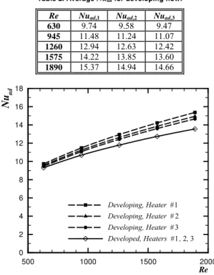
When the flow was uniform at the channel entrance, its development was distinct along each heater in the channel, so that the average Nusselt number of each one depended on its position. Considering only a single active heater, the average Nu values were also independent of the three reference temperatures, due to their coincidence. Table 2 presents the average Nusselt number for each heater in this case, indicating the Reynolds number and position dependence. Due to the simultaneous thermal and velocity boundary layer development over the heaters, the values in Table 2 are larger than the corresponding values in Table 1. In addition, the upstream heaters present larger values than those downstream. The average Nu results for a single active heater are presented in Fig. 2 for the five tested values of Re. The curves for the three heaters coincide when the flow is developed from the channel entrance, and they are distributed when the flow is developing along the channel. Under developing flow, the curves for the downstream heaters tend to that for the developed flow.
Another parameter obtained from the simulations for a single active heater was the influence coefficient g*(n–n), as defined in Eq. (3). When the flow was developed from the channel entrance, the velocity profile over any heater was invariant and the coefficient g*(n–n) was independent of the heater position – it changed only with the Reynolds number. The results corresponding to Pr = 0.7 are indicated as g*(0) in Table 3. The values increase with Re, mainly due to larger mass flow rate in the channel. For the developing flow, the influence of Re on the coefficients g*(n–n) presented the same trend. In addition, these coefficients also depended on the heater position, increasing downstream mainly due to the velocity boundary layer development and a higher heater average temperature. These results are presented in Table 3 as g*(1–1), g*(2–2) and g*(3–3). The results of Table 3 are also presented in Fig. 3, showing the observed trends.
Table 2. Average Nuad for developing flow.
Re Nuad,1 Nuad,2 Nuad,3
630 9.74 9.58 9.47
945 11.48 11.24 11.07
1260 12.94 12.63 12.42
1575 14.22 13.85 13.60
1890 15.37 14.94 14.66
Re
N
u
ad500 1000 1500 2000
0 2 4 6 8 10 12 14 16 18
Developing, Heater# 1
Developing, Heater# 2
Developing, Heater# 3
Developed, Heaters # 1,2,3
Figure 2. Average Nuad for a single active heater (Pr = 0.7).
Table 3. g*(n–n) for developed and for developing flow.
Developed
flow Developing flow
Re
g*(0) g*(1-1) g*(2-2) g*(3-3)
630 23.684 22.639 23.017 23.284
945 30.940 28.811 29.426 29.878
1260 37.405 34.080 34.917 35.507
1575 43.269 38.766 39.801 40.533
1890 48.783 43.038 44.277 45.123
Re
g
*
(
n-n
)
500 1000 1500 2000
20 24 28 32 36 40 44 48 52
g*(0)
g*(1−1)
g*(2−2) g*(3−3)
Figure 3. g*(n–n) for developed and for developing flow.
Two or Three Active Heaters
The simulations for this case were performed initially with only two active heaters, dissipating the same heat flux. Again, the flow was considered either developed or with a uniform velocity at the channel entrance. The main purpose of these tests was to obtain the influence coefficients g*(n–i), as defined in Eq. (5). For developed channel flow, the coefficients g*(2–1) and g*(3–2) depended only on the Reynolds number and they were equal, due to the adopted geometry with the same heater length Lh and spacing Ls. They are represented by g*(1) in Table 4. The coefficient g*(3–1) indicates the adiabatic temperature rise of heater 3 above the channel flow inlet temperature due to the heat flux on heater 1 and it is indicated as g*(2) in Table 4. These coefficients increase with Re due to larger flow rates and the values of g*(1) are larger than those of g*(2) because the former represent the influence of a closer upstream heater. For a developing flow from a uniform velocity at the channel inlet, these coefficients depended on the heater position. They increased at downstream positions mainly due to the velocity boundary layer development and far downstream they would equal the values attained by the developed flow, indicated by g*(1) and g*(2). The results of g*(n–i) presented in Table 4 are also indicated in Fig. 4, showing the indicated trends. The values of the average Nuad obtained from these simulations were identical to those presented in Fig. 2 and Tables 1 and 2, for the developed and for the developing flow.
Table 4. g*(n–i) for developed and for developing flow.
Developed flow Developing flow
Re
g*(1) g*(2) g*(2-1) g*(3-2) g*(3-1)
630 7.208 4.540 7.060 7.123 4.477
945 9.411 5.905 8.974 9.084 5.678
1260 11.282 7.048 10.638 10.798 6.741
1575 13.069 8.162 12.126 12.332 7.646
Re
g
*
(
n-i
)
500 1000 1500 2000
0 2 4 6 8 10 12 14 16
g*(1)
g*(2)
g*(2-1)
g*(3-2)
g*(3-1)
Figure 4. g*(n–i) for developed and for developing flow.
The simulations involving three active heaters comprised the case with the same heat flux from the heaters and two cases with distinct heat fluxes. Considering the heaters indicated in Fig. 1, the first heat flux distribution wasq1′′=q2′′=q3′′, corresponding to a ratio equal to 1-1-1 (case 1). For the other two cases, with distinct heat fluxes, the corresponding distribution ratios were equal to 5-3-1 (case 2) and to 3-5-1 (case 3).
For developed flow, the numerical average Nusselt numbers are presented in Table 5. The average Nuad were in fact a function of just the Reynolds number. There were identical to those presented in Table 1 for a single active heater in the channel and were invariant with position and the distinct thermal conditions. For the heater in the first row (#1), the average Num and Nuin are also the same as Nuad, due to the coincidence of the reference temperatures. For the downstream heaters (#2 and #3), the values of the average Num and Nuin changed with the thermal conditions, as indicated in Table 5. For these two rows, since Tin< Tm< Tad , the results for the average Nu follow Nuin< Num< Nuad .
Table 5. Average Nusselt numbers for developed flow.
Case 1:
1-1-1
Case 2:
5-3-1
Case 3:
3-5-1
All cases Re
Num Nuin Num Nuin Num Nuin Nuad
1 9.31 9.31 9.31 9.31 9.31 9.31 9.31
2 7.38 7.14 6.48 6.18 8.05 7.88 9.31
630
3 6.59 6.22 3.67 3.24 3.37 3.01 9.31
1 10.69 10.69 10.69 10.69 10.69 10.69 10.69
2 8.42 8.20 7.37 7.10 9.20 9.05 10.69
945
3 7.49 7.16 4.11 3.74 3.78 3.46 10.69
1 11.79 11.79 11.79 11.79 11.79 11.79 11.79
2 9.25 9.06 8.08 7.84 10.12 9.98 11.79
1260
3 8.20 7.91 4.48 4.14 4.12 3.83 11.79
1 12.74 12.74 12.74 12.74 12.74 12.74 12.74
2 9.96 9.78 8.70 8.47 10.91 10.78 12.74
1575
3 8.82 8.55 4.79 4.47 4.41 4.14 12.74
1 13.56 13.56 13.56 13.56 13.56 13.56 13.56
2 10.59 10.42 9.24 9.03 11.60 11.48 13.56
1890
3 9.36 9.10 5.07 4.77 4.67 4.42 13.56
Re
N
u
500 1000 1500 2000
0 4 8 12 16 20 24 28
Num, case1-1-1
Nui n, case1-1-1
Num, case5-3-1
Nui n, case5-3-1
Num, case3-5-1
Nui n, case3-5-1
Nua d, all cases
Figure 5. Average Nu for heater #3 – all cases – developed flow.
Thus, it is evident the advantage and convenience to use Nuad. It is an invariant descriptor of the convective heat transfer, independent of the thermal conditions. It may also be obtained under simple conditions, as that with a single active heater in the channel. The results of Table 5 for the heater #3 are also presented in Fig. 5, showing the changes of the average Nuad, Num and Nuin for the three cases considered in the simulations.
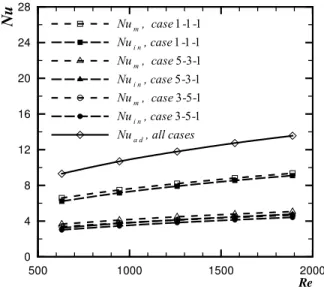
For the developing flow, the average Nusselt numbers are indicated in Table 6. The average Nuad are the same as those presented in Table 2, indicating again the invariant nature of this parameter. The average values of Nuin and Num change with the thermal conditions, as can be observed in Table 6. The values for the first row (heater #1) are the same as those of Nuad due to the mentioned coincidence of the reference temperatures for his row. The values presented in Table 6 for the heater #3 are also shown in Fig. 6, indicating again the invariant description of the convective heat transfer made by Nuad, while the values associated to the other two definitions change with the thermal conditions.
Table 6. Average Nusselt numbers for developing flow.
Case 1:
1-1-1
Case 2:
5-3-1
Case 3:
3-5-1
All cases Re
Num Nuin Num Nuin Num Nuin Nuad
1 9.74 9.74 9.74 9.74 9.74 9.74 9.74
2 7.59 7.33 6.67 6.34 8.28 8.09 9.58
630
3 6.71 6.32 3.74 3.29 3.43 3.05 9.47
1 11.48 11.48 11.48 11.48 11.48 11.48 11.48
2 8.85 8.61 7.75 7.45 9.67 9.50 11.24
945
3 7.76 7.41 4.26 3.86 3.92 3.58 11.07
1 12.94 12.94 12.94 12.94 12.94 12.94 12.94
2 9.90 9.68 8.66 8.38 10.84 10.68 12.63
1260
3 8.64 8.32 4.72 4.35 4.34 4.03 12.42
1 14.22 14.22 14.22 14.22 14.22 14.22 14.22
2 10.83 10.62 9.46 9.20 11.87 11.71 13.85
1575
3 9.43 9.11 5.12 4.77 4.71 4.41 13.60
1 15.37 15.37 15.37 15.37 15.37 15.37 15.37
2 11.67 11.47 10.19 9.93 12.79 12.64 14.94
1890
Re
N
u
500 1000 1500 2000
0 4 8 12 16 20 24 28
Num, case1-1-1
Nui n, case1-1-1
Num, case5-3-1
Nui n, case5-3-1
Num, case3-5-1
Nui n, case3-5-1
Nua d, all cases
Figure 6. Average Nu for heater #3 – all cases – developing flow.
The heaters average wall temperature above the inlet flow temperature, as predicted by Eq. (6), was expressed in the dimensionless form defined by Eq. (15).
(
) ( )
(
) ( )
2 n s 2 i s
n
i
q q q q
g n n g n i
Re Pr Re Pr
∗ ∗
′′ ′′ ′′ ′′
θ = − +
∑
− (21)The heat flux qs′′ indicates the heaters smallest heat flux and it is used as the reference in the definition of the dimensionless temperature. The influence coefficients g* were those presented in Tables 3 and 4.
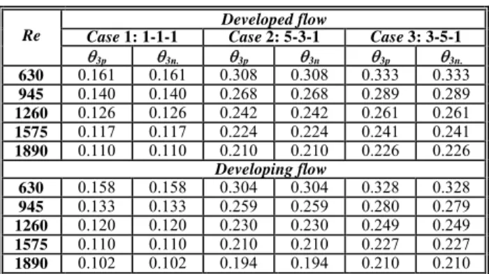
The numerical results from the simulations for the three considered cases were compared with the predictions of Eq. (21). The results for the heater #3 are presented in Table 7 for developed and for developing flow. For the three active heaters, the agreement was always within 0.1%.For each case the average θ3 decreases with Re, as indicated by Eq. (21). For the developed flow, the values are greater than those for the developing flow due to the corresponding larger influence coefficients g* indicated in Tables 3 and 4.
The numerically obtained dimensionless temperature distributions along each heater for case 2 (heat flux ratios 5-3-1) under developed flow and Re = 1890 are presented in Fig. 7, together with their average values. The corresponding distributions of the adiabatic dimensionless temperature and their average values are also included in Fig. 7. They indicate the expected increase of the heaters temperature in the flow direction and the corresponding decrease of their adiabatic surface temperature. The average temperatures obtained for each heater are those employed in the definition of the adiabatic heat transfer coefficient. It should be noted that the adiabatic surface temperature for heater #1 is coincident with Tin, so that its dimensionless temperature, as defined by Eq. (18), is equal to zero.
Table 7. Numerical and predicted average θ of heater #3.
Developed flow
Case 1: 1-1-1 Case 2: 5-3-1 Case 3: 3-5-1
Re
θ3p θ3n. θ3p θ3n θ3p θ3n. 630 0.161 0.161 0.308 0.308 0.333 0.333
945 0.140 0.140 0.268 0.268 0.289 0.289
1260 0.126 0.126 0.242 0.242 0.261 0.261
1575 0.117 0.117 0.224 0.224 0.241 0.241
1890 0.110 0.110 0.210 0.210 0.226 0.226
Developing flow
630 0.158 0.158 0.304 0.304 0.328 0.328
945 0.133 0.133 0.259 0.259 0.280 0.279
1260 0.120 0.120 0.230 0.230 0.249 0.249
1575 0.110 0.110 0.210 0.210 0.227 0.227
1890 0.102 0.102 0.194 0.194 0.210 0.210
x/Lh
θ
10.20 0.40 0.60 0.80 1.00
0.00 0.10 0.20 0.30 0.40 0.50
x/Lh
θ
20.20 0.40 0.60 0.80 1.00
0.00 0.10 0.20 0.30 0.40
x/Lh
θ
30.20 0.40 0.60 0.80 1.00
0.00 0.04 0.08 0.12 0.16 0.20 0.24 0.28
Figure 7. Distribution of θ for developed flow in case 2.
Conclusions
Numerical simulations of the laminar convective heat transfer from three discrete heaters flush mounted to a single wall of a channel showed that the average Nuad for each heater is independent
Re = 1890 Case 2:5-3-1
Re = 1890 Case 2:5-3-1
Re = 1890 Case 2:5-3-1
w θ
w θ
w θ
ad θ
ad θ w
θ
w θ
w θ
ad θ
of their heat flux distribution. Comparatively, the evaluated average values of Num and Nuin change with the heat flux distribution. This result is quite important, because the Nuad predictions can be made under much simpler conditions, like that with a single active heater in the channel and the results can be applied to any other thermal condition. In addition, it was shown that the heaters average temperature under any thermal conditions can be predicted using the influence coefficients g* and the superposition principle, since the energy equation is linear. These coefficients can be obtained from simulations with a single active heater and with two active heaters having the same heat flux. The resulting values can then be applied to predict the average heaters temperatures for any other thermal condition with three active heaters. The present work was performed with three heater rows, but the method can be extended to a larger number of rows.
Acknowledgements
The support of CNPq (Brazilian Research Council) for the first author in the form of a doctorate program scholarship is gratefully acknowledged.
References
Anderson, A. and Moffat, R.J., 1992a, “The Adiabatic Heat Transfer Coefficient and the Superposition Kernel Function: Part I – Data for Array of Flatpack for Different Flow Conditions”, Journal of Electronics Packaging, Vol. 114, pp. 14-21.
Anderson, A. and Moffat, R.J., 1992b, “The Adiabatic Heat Transfer Coefficient and the Superposition Kernel Function: Part II – Modeling Flatpack Data as a Function of Turbulence”, Journal of Electronics Packaging, Vol. 114, pp. 22-28.
Arvizu, D. and Moffat R.J., 1982, “The Use of Superposition in Calculating Cooling Requirements”, Proceedings of the Electronics Cooling Conference IEEE, San Diego, CA, USA, pp. 133-144.
Arvizu, D., Ortega, A. and Moffat, R.J., 1985, In: Oktay, S. and Moffat R.J. (Eds.), “Cooling Electronic Components: Forced Convection Experiments with an Air-Cooled Array”, Electronics Cooling, ASME, New York, USA.
Bejan, A., 1995, “Convective Heat Transfer”, 2nd ed., John Wiley & Sons Inc., New York, USA, 623p.
De Vahl Davis, G., 1983, “Natural Convection of Air in a Square Cavity: A Benchmarck Numerical Solution”, International Journal for Numerical Methods in Fluids, Vol. 3, pp. 249-264.
Incropera, F.P., Kerby, J.S., Moffat, D.F. and Ramadhyani, S., 1986, “Convection Heat Transfer from Discrete Heat Sources in a Rectangular Channel”, International Journal of Heat and Mass Transfer, Vol. 29, pp. 1051-1058.
Kays, W.M. and Crawford, M.E., 1993, “Convective Heat and Mass Transfer”, 3rd ed., McGraw-Hill, New York, USA, 601p.
Mahaney, H.V., Incropera, F.P. and Ramadhyani, S., 1990, “Comparison of Predicted and Measured Mixed Convection Heat Transfer from an Array of Discrete Sources in a Horizontal Rectangular Channel”, International Journal of Heat and Mass Transfer, Vol. 33, pp. 1233-1245.
Moffat, R.J., 1998, “What’s New in Convective Heat Transfer?”,
International Journal of Heat and Fluid Flow, Vol. 19, pp. 90-101.
Moffat, R.J., 2004, “hadiabatic and u’max”, Journal of Electronics Packaging, Vol. 126, pp. 501-509.
Patankar, S.V., 1980, “Numerical Heat Transfer and Fluid Flow”, Hemisphere Publishing Corporation, New York, USA, 197p.
Ortega, A. and Lall, B.S., 1992, “A Clarification of the Adiabatic Heat Transfer Coefficient as Applied to Convective Cooling of Electronics”, Proceedings of the 8th Annual IEEE Semiconductor Thermal Measurement and Management Symposium, Austin, TX, USA, pp. 1-3.