Influence of the choice of the inlet turbulence intensity on the performance of numerically simulated moderate Reynolds jet flows – Part 1 – the near exit region of the jet

Influence of the choice of the inlet turbulence intensity on

the performance of numerically simulated moderate

Reynolds jet flows

–

Part 1

–

the near exit region of the jet

Radu DOLINSKI

, Florin BODE

, Ilinca NASTASE*

, Amina MESLEM

,

Cristiana CROITORU

*Corresponding author

CAMBI, Technical University of Civil Engineering in Bucharest, Building Services

Department, 66 Avenue Pache Protopopescu, 020396, Bucharest, Romania,

ilinca.nastase@cambi.ro*, cristiana.croitoru@cambi.ro

Wind Engineering and Aerodynamics Laboratory, Technical University of Civil

Engineering of Bucharest, 020396 Bucharest, Romania,

radu.dolinski@gmail.com

Technical University of Cluj-Napoca, Mechanical Engineering Department,

103-105 Muncii, D03, Cluj-Napoca, Romania

florin.bode@termo.utcluj.ro

LaSIE Laboratory, University of La Rochelle,

Av. Michel Crépeau, 17000, La Rochelle, France

amina.meslem@univ-lr.fr

DOI: 10.13111/2066-8201.2013.5.4.3

Abstract: A real problem when trying to develop a numerical model reproducing the flow through an

orifice is the choice of a correct value for the turbulence intensity at the inlet of the numerical domain in order to obtain at the exit plane of the jet the same values of the turbulence intensity as in the experimental evaluation. There are few indications in the literature concerning this issue, and the imposed boundary conditions are usually taken into consideration by usage without any physical fundament. In this article we tried to check the influence of the variation of the inlet turbulence intensity on the jet flow behavior. This article is focusing only on the near exit region of the jet. Five values of the inlet turbulence intensity Tu were imposed at the inlet of the computational domain, from 1.5% to 30%. One of these values, Tu= 2% was the one measured with a hot wire anemometer at the jet exit plane, and another one Tu= 8.8% was issued from the recommendation of Jaramillo [1]. The choice of the mesh-grid and of the turbulence model which was the SST k-ω model were previously established [2]. We found that in the initial region of the jet flow, the mean streamwise velocity profiles and the volumetric flow rate do not seem to be sensitive at all at the variation of the inlet turbulence intensity. On the opposite, for the vorticity and the turbulent kinetic energy (TKE) distributions we found a difference between the maximum values as high as 30%. The closest values to the experimental case were found for the lowest value of Tu, on the same order of magnitude as the measurement at the exit plane of the jet flow. Mean streamwise velocity is not affected by these differences of the TKE distributions. Contrary, the transverse field is modified as it was displayed by the vorticity distributions. This observation allows us to predict a possible modification of the entire mean flow field in the far region of the jet flow.

1. INTRODUCTION

The lobed orifices and nozzles are commonly used under very high Reynolds number in aeronautics and combustion applications for thrust improvement and noise reduction [3-5]. Under low or moderate Reynolds numbers for heating, ventilation and air conditioning (HVAC) applications, the analysis of lobed nozzle and orifice jets shows that large streamwise structures generated by the lip of the lobed diffuser are present and control the ambient air induction [6-11]. At each elementary cross-shaped orifice of a perforated panel diffuser [10], large scale structures develop in the orifice troughs and control air entrainment in the jet near field [6, 7]. The total entrainment of the perforated panel is depending on the interactions between neighboring jets [12] as well as on the geometrical parameters of the elementary orifice. Improving the entrainment at the scale of an elementary lobed jet is one of the parts of the optimization problem [10]. During this process we aim for the same inlet volume flow rate to obtain a maximum ambient-air entrainment without reducing the jet’s throw (i.e. downstream penetration).

The present article was developed during the calibration process of our numerical models for thelobed orifice jet simulation. Through this simulation we aim to optimize the geometry of the lobed orifice in terms of jet’s throw and self-induction. In previous studies [2, 12] we compared the quality of seven Reynolds Averaged Navier-Stokes (RANS) modelsto provide the cross-shaped jet flow characteristics both in elementary and twin-jet configuration at moderate Reynolds number. Recent experimental data for a turbulent cross-shaped jet [13] were used to assess the capability and limits of these turbulence models to provide near field orifice lobed jet characteristics at moderate Reynolds number [2].

2. EXPERIMENTAL AND NUMERICAL METHODS

a) Experimental facility and methods

The air jet considered in the present investigation is generated using a cross-shaped orifice in the center of a circular aluminum plate of 94 mm diameter and of 1.5 mm thickness. The equivalent diameter of the cross orifice is 10 mm. The equivalent diameter was defined as

  4A₀

D_e where A0 is the exit area of the orifice.The plane bisecting the width of the

lobes is referred to as the major plane (MP), and the plane bisecting opposing troughs is referred to as the minor plane (mP). Both the major and minor planes are perpendicular to the aluminumplate containing the orifice(Fig. 1a). The air jet experimental facility (Fig 1 b) consists of an axial miniature fan placed inside a 1 m long metallic pipe of 0.16 m diameter. A convergent duct placed at the end of the pipe ensures the reduction of the turbulence level at the jet exit and a honeycomb structure was positioned just upstream of the convergent duct. A time-resolved stereoscopic PIV system used for this study is composed of two

Phantom V9 cameras of 1200×1632 pixels2

, a synchronizer and an Nd: YLF NewWave Pegasus laser of 10 mJ energy and 527 nm wavelength. The LaVision DaVis 7 software is used for data acquisition, processing and post-processing. The acquisition frequency of the PIV system is 500 Hz for a maximal image window. In each plane, a number of 500 image couples were acquired. The air jet flow was seeded with small olive oil droplets, 1–2 μm in

diameter, provided by a liquid seeding generator. The final grid was composed of 32 x 32 pixels interrogation deforming windows with 50% overlapping leading to a spatial resolution of 0.59 mm. The maximal displacement errors are equal to 1%, 2%, and 2.5% for the longitudinal, vertical, and transversal directions, respectively. The rms PIV velocity error is about 0.09 m/s. The absolute value of the bias vorticity error is 0.8%, and the random

vorticity error is estimated as ±1.5% at the 95% confidence level. The error for the turbulent

kinetic energy is estimated as ±4.2%. In the experimental case and in all numerical cases the

volumetric flow rate was 3.3×10-4

m3/s leading to a Reynolds number Re0mean= 2676. The turbulent intensity profile is flat, with about 2% in the central region for both the minor plane (mP) and the major plane (MP) defined in Fig. 1 (a). In the regions of the shear layer, the turbulence intensity increases in both planes. This increase is about 15% for the minor and the major planes.

a) b)

Fig. 1 a) Investigated cross-shaped orifice [2], b) Air jet facility

b) Numerical model

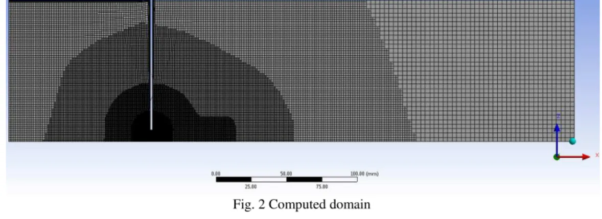
symmetry of the problem, just one fourth of the domain was modeled (so the dimension becomes 10De in the Y and Z directions). Since the orifice plate had a finite thickness (0.15De), the inlet plane of the jet was set at X = - 0.15De and the outlet plane of the jet at X = 0 (see Fig 2).

Fig. 2 Computed domain

Fig. 3 Mesh in the cross shaped orifice zone (streamwise and transverse section)

From our previous experience [12, 14] we tried to achieve a final grid that would try to meet all necessary requirements for a good mesh, such as: the minimum number of cells needed in the critical section (30 cells), the smallest cell size (0.01mm), the largest cell size (2mm), y+ (less than 4 and its mean value was 1.3), the rate of cell growth (1.05), skewness of the cells. The resulted grid had a size of 4 million Cartesian non-uniform cells and all the simulation were performed using the same grid. This type of grid has been successfully used in our previous researches and managed to solve the flow field of different type of cross-shaped jets. Nevertheless, a Cartesian grid is the best choice for flows with a strong velocity component in one direction such as jet flows. Results were compared with the experimental data of the turbulent cross-shaped jet [13] at moderate Reynolds number and the results of the comparison was satisfactory convincing us that we have a good quality mesh.

In this article results are presented only for the SST k-ω model. A mesh dependency study was performed for this model and results are presented in [2].

intensity at the inlet of the numerical domain in order to obtain at the exit plane of the jet the same values of the turbulence intensity as in the experimental evaluation.

There are several recommendations in the literature for choosing values of the turbulence intensity at the inlet [1]. For internal flows the value of turbulence intensity can be fairly high with values ranging from 1% - 10% being appropriate at the inlet. The turbulence intensity at the core of a fully developed duct flow can be estimated as:

8 / 1 Re 16 . 0  

Tu [1].

In our case, this relation gives a value of Tu = 8.8 % for a fully developed flow at the inlet. We tried to check the influence of the variation of the turbulence intensity at the inlet by imposing several values. The first one was of 2% and was inspired by the low turbulence intensity measured at the jet exit. Other values of 1.5%, 5%, 8.8%, 10% and 30% were tested. The SIMPLE algorithm was used for pressure-velocity coupling. The flow variables were calculated on a collocated grid. A second order upwind scheme was used to calculate the convective terms in the equations, integrated with the finite volume method. Computations were performed on a SGI Altix Ice cluster. For each computation presented in this paper, 24 processors were used.

Regarding the accuracy of results for the cases studied, the imposed convergence criterion was 10-5 for all the variables residuals. Both of the above criteria were met before we declared our solution to be converged.

3. RESULTS AND DISCUSSION

As we mentioned earlier, one of the first step that we wanted to check was related to the choice of the inlet turbulence intensity in order to obtain close to the jet exit, at X=0.1De (X= 0 is the plane of the jet exit) a value that would be close to the one measured using HWA, which was Tu0.1De = 2%. This way in Fig. 4 is presented the streamwise evolution of the turbulence intensity on the flow axis (Y= 0 and Z= 0) for the entire computational domain (Fig. 4 a) and in close to the jet exit region (Fig. 4 b). The first value of Tu = 2% that we tested displays at X=0.1De a value of Tu0.1De = 1.97%. If we try the recommendation of Jaramillo [1] of imposing a Tu= 8.8%, the obtained value is Tu0.1De = 3.19%. For the other testes values we obtained respectively: Tu0.1De = 1.96 % for Tu=1.5%; Tu0.1De = 3.82 for Tu=10% and Tu0.1De = 12.6% for Tu = 30%. This way, the closest values to the experimental data were obtained for Tu=1.5% and 2%.

a) b)

Fig. 4 Streamwise evolution of the turbulence intensity on the flow axis: a) entire computational domain, b) close to the jet exit region

0 10 20 30 40 50 60 70 80 90

-15 -10 -5 0 5 10 15 20 25

Tu 1.5%

Tu 2%

Tu 8.8%

Tu 10%

Tu 30% e D X [%] Tu 0 2 4 6 8 10 12 14 16 18 20

-2 -1 0 1 2

a) b)

c)

Fig. 5 Evolution of the streamwise velocity on the jet axis: a) from the jet exit to the end of the computational domain, b) close to the jet exit region; c) Evolution of the volumetric flow rates

Major Plane Minor Plane

a) b) 0 0.2 0.4 0.6 0.8 1 1.2

0 10 20 30

Tu 1.5% Tu 2% Tu 8.8% Tu 10% Tu 30% Experimental e D X JC JC U U 0 4.8 4.85 4.9 4.95 5 5.05 5.1 5.15 5.2 5.25 5.3

0 1 2 3 4 5

Tu 1.5% Tu 2% Tu 8.8% Tu 10% Tu 30% e D X JC U 1.0 1.5 2.0 2.5

0 1 2 3 4 5

PIV Tu 1.5% Tu 2% Tu 8.8% Tu 10% Tu 30% 0 Q Q e D X -0.5 0.5 1.5 2.5 3.5 4.5 5.5

-1.5 -1 -0.5 0 0.5 1 1.5

Tu 1.5 % Tu 2% Tu 10% Tu 30%

] / [ms U e D Y/ -0.5 0.5 1.5 2.5 3.5 4.5 5.5

-1.5 -1 -0.5 0 0.5 1 1.5

Tu 1% Tu 2% Tu 10% Tu 30% e D Z/ ] / [m s U -0.5 0.5 1.5 2.5 3.5 4.5 5.5

-1.5 -1 -0.5 0 0.5 1 1.5

Tu 1.5% Tu 2% Tu 10% Tu 30% ] / [ms U e D Y/ -0.5 0.5 1.5 2.5 3.5 4.5 5.5

-1.5 -1 -0.5 0 0.5 1 1.5

Tu 1.5% Tu 2% Tu 10% Tu 30% ] / [m s U

e

c)

d)

Fig. 6 Streamwise velocity profiles in the Major and Minor planes for different values of Tu: a) X=0.1De, b) X=1De, c) X=3De, d) X=5De

We wanted to see what is the influence of this parameter on two global quantities that are very important from the point of view of HVAC application, namely the streamwise decay of the axial velocity and the volumetric flow rate evolution. The first one is related to the jet throw and the second one to the capability of induction of a jet flow generated by a given air diffuser.

Fig. 5 shows the axial evolutions of these quantities. The numerical results predicted by the SST-k- turbulence model are compared with the HWA measurements (Fig. 5a) for all the tested values of the inlet turbulence intensity. Fig. 5a displays the normalized streamwise velocity from the jet exit to the end of the computational domain while Fig. 5b gives a focus on the near exit region and the axial velocity in this subfigure was presented with its absolute values. As we showed in [2] all tested RANS models fail in predicting a good evolution of centerline velocity in the full observed axial distance. The nearest jet core length to experimental data was given by the SST-k- turbulence model. Fig. 5b shows that the streamwise velocity on the jet axis, in the near and far fields, is not sensitive to thetested values of Tu.

a) -0.5 0.5 1.5 2.5 3.5 4.5 5.5

-1.5 -1 -0.5 0 0.5 1 1.5

Tu 1.5% Tu 2% Tu 10% Tu 30% ] / [ms U e D Y/ ] / [ms U e D Y/ -0.5 0.5 1.5 2.5 3.5 4.5 5.5

-1.5 -1 -0.5 0 0.5 1 1.5

Tu 1.5% Tu 2% Tu 10% Tu 30% ] / [ms U e D Y/ -0.5 0.5 1.5 2.5 3.5 4.5 5.5

-1.5 -1 -0.5 0 0.5 1 1.5

Tu 1.5% Tu 2% Tu 10% Tu 30% ] / [ms U e D Y/ ] / [ms U e D Y/ ] / [ms U e D Y/ -0.5 0.5 1.5 2.5 3.5 4.5 5.5

-1.5 -1 -0.5 0 0.5 1 1.5

Tu 1.5% Tu 2% Tu 10% Tu 30% ] / [m s U

e

b)

c)

d)

e) Fig. 7 In plane velocity fields and streamwise vorticity distributions for two extreme values of the imposed Tu

a)

b)

c)

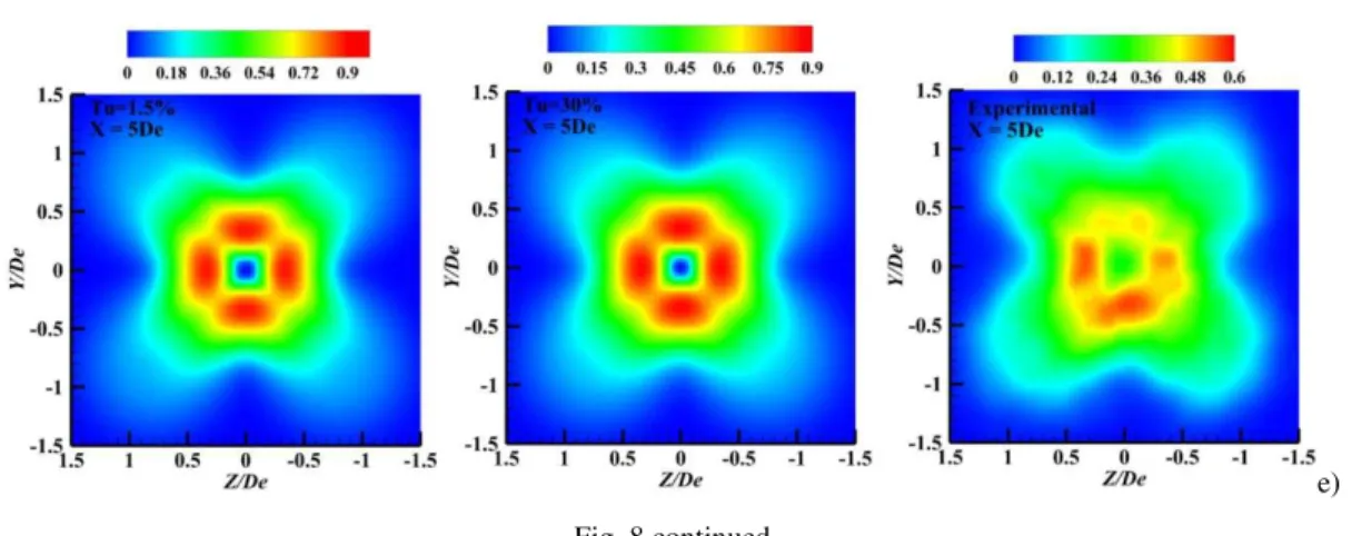
d) Fig. 8 Turbulent kinetic energy distributions for two extreme values of the imposed Tu and of the experimental

e)

Fig. 8 continued

The ambient air induction (Fig. 5c) is obtained by integrating the streamwise velocity in the cross-planes, considering a threshold value of 0.15 m/s. As our particular application is directly interested in quantifying the mixing between jets generated by HVAC terminal units and their ambience, we considered the 0.15 m/s criterion defining the extinction of the flow from the point of view of the thermal and draft comfort of the occupants [15]. As for the streamwise velocity decay, we found that the volumetric flow rates are not sensitive to the initial turbulence intensity at all in the near exit region of the jet flow. This result is in accordance with Fig. 6 which presents the streamwise velocity profiles at different axial positions for both major and minor planes.

Physical phenomena, such as, axis-switching and entrainment in the near field of the cross-shaped jet are interrelated with vortices development in this region [13]. Self induction deformation of primary vortices and secondary vortices development govern the mean velocity field.

Within the X-range of stereoscopic PIV measurements (0.5 De ≤ X ≤ 5 De), the

streamwise component of the normalized vorticity is defined as:

mean e X

U D Z V Y W

0

   

 

     

 .

Fig. 7 presents its distributions in the streamwise planes for the experimental case and for two numerical cases corresponding to Tu=1.5% and 30%. To facilitate the observation of the jet flow dynamics, the in-plane vector field is also represented on the plots. The four regions of counter-rotating outflow vortices pairs from the jet center in the diagonal direction are specific to this type of orifice jet [2, 13].

By examining the shape and intensity of the main vortices pairs for both simulated flows we can observe a slight difference on the maximum values which amplifies beginning with X=2De. At this distance, the maximum values of the streamwise vorticity were ωX =1.95 for

Tu=1.5% and ωX =1.65 for Tu=30%, respectively, which is translated through a relative difference of 14%. At X=5De the maximum values of the streamwise vorticity were ωX =0.25

for Tu=1.5% and ωX =0.15 for Tu=30% respectively, which is translated through a relative difference as high as 30%.The Tu=1.5% case gives overall values of the streamwise vorticity closer to the experimental case than the Tu=30%.

fields and for the same values of Tu=1.5% and 30%. As expected, an obvious difference is found between the two cases from the exit plane of the jet. It is very interesting to observe that the mean streamwise velocity is not affected by these differences of the TKE distributions.

Contrary, the transverse field is modified as it was displayed by the vorticity distributions. This observation allows us to predict a possible modification of the entire mean flow field in the far region of the jet flow.

Once again, as for the vorticity fields, the Tu=1.5% case gives overall values of the streamwise vorticity closer to the experimental case than the Tu=30%. Indeed, in Fig. 8 it may be observed that maximum TKE levels obtained for the experimental case are closer to the ones for the numerical simulation where Tu=1.5%.

4. CONCLUSIONS

One of the problems we encountered in our approach of developing numerical models which attempt to solve the flow through orifices or nozzles was the choice of a correct value for the turbulence intensity at the inlet of the numerical domain. The “correctitude” of this choice would be validated by obtaining for instance at the exit plane of the jet the same values of the turbulence intensity as in an experimental evaluation.

In this article we tried to determine the influence of the variation of the inlet turbulence intensity on the jet flow behavior. This article is focusing only on the near exit region of the jet. Five values of the inlet turbulence intensity Tu were imposed at the inlet of the computational domain, from 1.5% to 30%. One of these values, Tu= 2% was the one measured with a hot wire anemometer at the jet exit plane, and another one Tu= 8.8% was issued from the recommendation of Jaramillo [1]. The choice of the mesh-grid and of the turbulence model which was the SST k-ω model were previously established [2]. We found that in the initial region of the jet flow, the mean streamwise velocity profiles and the volumetric flow rate do not seem to be sensitive at all at the variation of the inlet turbulence intensity. On the opposite, for the vorticity and the turbulent kinetic energy (TKE) distributions we found a difference between the maximum values as high as 30%. The closest values to the experimental case were found for the lowest value of Tu, on the same order of magnitude as the measurement at the exit plane of the jet flow. Mean streamwise velocity is not affected by these differences of the TKE distributions. Contrary, the transverse field is modified as it was displayed by the vorticity distributions. This observation allows us to predict a possible modification of the entire mean flow field in the far region of the jet flow.

There are few indications in the literature concerning this issue, and the imposed boundary conditions are usually taken into consideration by usage without any physical fundament. In our case it was proven that choosing a value of the inlet turbulence intensity that was close to an experimental determination, even if that determination was not spatially matched with the boundary condition, was a better solution than an empirical recommendation from the literature.

ACKNOWLEDGEMENTS

REFERENCES

[1] J. E. Jaramillo, C. D. Perez-Segarra, I. Rodriguez and A. Oliva, Numerical study of plane and round impinging jets using RANS models, Numer. Heat Transfer Part B,54, 213-237, 2008.

[2] A. Meslem, F. Bode, C. Croitoru and I. Nastase, Comparison of turbulence models in simulating jet flow from a cross-shaped orifice, Accepted for publication by European Journal of Mechanics B Fluids, 2013. [3] H. Hu, T. Saga, T. Kobayashi and N. Taniguchi, A Study on a Lobed Jet Mixing Flow by Using Stereoscopic

Particle Image Velocimetry Technique, Physics of Fluids,13 (11), 3425-3441, 2001.

[4] E. J. Gutmark and F. F. Grinstein, Flow Control with Noncircular Jets, Annual Reviews of Fluid Mechanics,

31, 239-272, 1999.

[5] V. M. Belovich and M. Samimy, Mixing processes in a coaxial geometry with a central lobed mixer-nozzle,

AIAA Journal,35 (5), 1997.

[6] I. Nastase, A. Meslem and P. Gervais, Primary and secondary vortical structures contribution in the entrainement of low Reynolds number jet flows, Experiments in Fluids,44 (6), 1027-1033, 2008. [7] I. Nastase and A. Meslem, Vortex dynamics and mass entrainment in turbulent lobed jets with and without

lobe deflection angles, Experiments in Fluids,48 (4), 693-714, 2010.

[8] M. El-Hassan and A. Meslem, Time-resolved stereoscopic PIV investigation of the entrainment in the near-field of circular and daisy-shaped orifice jets, Physics of Fluids, 22 (035107), 26 p., 2010.

[9] A. Meslem, F. Bode, C. Croitoru and I. Nastase, Comparison of turbulence models in simulating jet flow from a cross-shaped orifice, European Journal of Mechanics B - Fluids in press (2013).

[10] A. Meslem, I. Nastase and F. Allard, Passive mixing control for innovative air diffusion terminal devices for buildings, Building and Environment,45, 2679-2688, 2010.

[11] I. Nastase, A. Meslem, V. Iordache and I. Colda, Lobed grilles for high mixing ventilation - An experimental analysis in a full scale model room, Building and Environment,46 (3), 547-555, 2011.

[12] A. Meslem, A. Dia, C. Beghein, M. El-Hassan and I. Nastase, A comparison of three turbulence models for the prediction of parallel lobed jets in perforated panel optimization, Building and Environment,46, 2203-2219, 2011.

[13] M. El-Hassan, A. Meslem and K. Abed-Meraïm, Experimental investigation of the flow in the near-field of a cross-shaped orifice jet, Phys. Fluids,23 (045101), 16 p., 2011.

[14] F. Bode, I. Nastase and C. Croitoru, Mesh dependency study using large eddy simulation of a very low reynolds cross-shaped jet, Mathematical modelling in civil engineering,4, 16-23, 2011.