www.geosci-model-dev.net/9/1383/2016/ doi:10.5194/gmd-9-1383-2016
© Author(s) 2016. CC Attribution 3.0 License.
Stride Search: a general algorithm for storm detection in
high-resolution climate data
Peter A. Bosler1, Erika L. Roesler2, Mark A. Taylor1, and Miranda R. Mundt3
1Sandia National Laboratories, Center for Computing Research, P.O. Box 5800, Albuquerque NM, 87185-1321, USA 2Sandia National Laboratories, Geophysics and Atmospheric Sciences, P.O. Box 5800, Albuquerque NM, 87185-0750, USA 3University of California Los Angeles, Department of Mathematics, P.O. Box 951555, Los Angeles CA, 90095-1555, USA
Correspondence to:Peter A. Bosler ([email protected])
Received: 26 June 2015 – Published in Geosci. Model Dev. Discuss.: 8 September 2015 Revised: 1 March 2016 – Accepted: 24 March 2016 – Published: 13 April 2016
Abstract. This article discusses the problem of identifying extreme climate events such as intense storms within large climate data sets. The basic storm detection algorithm is reviewed, which splits the problem into two parts: a spa-tial search followed by a temporal correlation problem. Two specific implementations of the spatial search algorithm are compared: the commonly used grid point search algorithm is reviewed, and a new algorithm called Stride Search is in-troduced. The Stride Search algorithm is defined indepen-dently of the spatial discretization associated with a partic-ular data set. Results from the two algorithms are compared for the application of tropical cyclone detection, and shown to produce similar results for the same set of storm identifi-cation criteria. Differences between the two algorithms arise for some storms due to their different definition of search re-gions in physical space. The physical space associated with each Stride Search region is constant, regardless of data res-olution or latitude, and Stride Search is therefore capable of searching all regions of the globe in the same manner. Stride Search’s ability to search high latitudes is demonstrated for the case of polar low detection. Wall clock time required for Stride Search is shown to be smaller than a grid point search of the same data, and the relative speed up associated with Stride Search increases as resolution increases.
1 Introduction
The identification of extreme events in climate data sets is a fundamental objective of many climate scientists. Data sets may be a reanalysis product or a particular model’s output,
and an extreme event may be any event classified as an im-portant deviation from a subjective normal state – loosely, a “storm”. End users of climate data and model developers alike frequently investigate prevalent storm tracks, intensity, or formation areas within a given data set, e.g., Williamson (1981), Hodges (1994), and Vitart et al. (1997). Annual means and statistical averages regarding the frequency of a particular type of storm in a particular region are another fre-quent subject of study, e.g., Sinclair (1994), Blender et al. (1997), Raible and Blender (2004), Bracegirdle and Gray (2008), and Kleppek et al. (2008). Individual storms’ struc-tures are often investigated to evaluate how well a model captures realistic physical features, e.g., Nordeng and Ras-mussen (1992), Walsh et al. (2007), Reed and Jablonowski (2011), and Føre et al. (2012). Common to all such efforts is the need to search data sets for quantifiable, objective storm identification criteria.
Identification criteria are defined as a small set of variables that together give a basic characterization of storms’ loca-tion, intensity, and size (Williamson, 1981; Hodges, 1994). Each variable is paired with a threshold value used to filter the data into a small number of categories. The particular variables and their appropriate threshold values vary greatly by application, and many studies have proposed and com-pared different sets of criteria; see Raible et al. (2008) and Neu et al. (2013) for a discussion of extratropical cyclone criteria. Walsh et al. (2007) and Horn et al. (2014) provide similar analyses for tropical cyclones.
spa-Algorithm 1Spatial search algorithm
Input: search domainR, storm identification criteria (spatial), data
Output: List of potential storms,L, organized by increasing time step
1:setL= empty list
2:for allfiles in data setdo
3: nT= number of time steps per file
4: Divide search domain into search sectors
5: fori= 1tonTdo
6: for allsearch sectors at time stepido
7: ifsector meets or exceeds identification criteriathen 8: setli= storm data at time stepi
9: addlitoL
10: end if
11: end for
12: end for
13:end for
tially defined identification criteria are met or exceeded. Sec-ond, a temporal correlation procedure correlates detection points across adjacent time steps to construct storm tracks and apply temporally defined identification criteria.
In comparison to the number of studies concerned with identification criteria, literature regarding the analysis of spa-tial search algorithms is relatively sparse in the climate com-munity. Such a discussion is of heightened importance due the growth of climate data sets in both size and number. As models and reanalysis products increase spatial and temporal resolution, and as ensembles are more commonly used fore-casting tools, the need to efficiently and accurately search cli-mate data sets is also increasing. Of equal concern to an algo-rithm’s performance is its ability to produce repeatable, ob-jective analysis of data (Hodges, 1994), regardless of the data layout and resolution. Contemporary models can incorporate advanced features such as variable resolution using unstruc-tured grids (e.g., Zarzycki and Jablonowski, 2014) and fre-quently employ different representations of the sphere than a traditional latitude–longitude grid (e.g., Putnam and Lin, 2007; Neale et al., 2012; Skamarock et al., 2012). An ideal search algorithm would be agnostic to such details.
In such an ideal world, the choice of search algorithm would not affect the statistics associated with a particular data set. In practice, however, we find that just as a change to the identification criteria of a particular storm type can change the statistics found in a particular data set (Raible et al., 2008; Horn et al., 2014), the way that data set is divided and searched – independently of the identification criteria – can also affect the statistics.
One contributing factor is that some of the variables used to identify storms, such as vorticity, have a dependence on the scale of the data (Sinclair, 1997; Walsh et al., 2007). This dependence may also vary with location depending on the layout of the data set. On a uniform latitude–longitude grid,
for example, the spatial scale of adjacent grid points varies with latitude. A search algorithm that does not account for this variation may inadvertently allow nonphysical artifacts related to data resolution and grid type to influence its out-put. Researchers may interpolate a data set to a different type of grid (Sinclair, 1994; Bracegirdle and Gray, 2008), em-ploy a spatial smoothing procedure (Sinclair, 1997), or ad-just threshold values as data resolution changes (Walsh et al., 2007) to alleviate some of these problems. We propose an al-ternative approach that separates the definition of an extreme event from its discrete representation in a data set.
The goal of this work is to provide an algorithm that allows identification criteria to be defined independently of the spa-tial resolution and layout of the data. The Stride Search algo-rithm facilitates searching data given on general unstructured grids as well as uniform latitude–longitude grids without al-teration, and provides improved performance over the com-monly used grid point search algorithm. Additionally, Stride Search treats all regions of the globe in the same manner, which allows users to search all latitudes, including the poles, efficiently. By decoupling the choice of identification criteria from the resolution and layout of the data, we aim to provide a robust objective search algorithm.
2 Storm detection algorithms
Algorithm 2Temporal correlation algorithm
Input: ListLof potential storms from spatial search output, max storm travel speedUmax, minimum duration tmin, other storm identification criteria (temporal)
Output: ListTof storm tracks
1:setT= empty list
2:NT= total number of time steps in data set
3:fori= 1toNTdo
4: for allelementsli∈Lat time stepido 5: start new tracktatli
6: continue =True 7: j=i
8: while continue do
9: examine alllj+1∈Lat time stepj+ 1for possible successors to stormlj
10: if successor foundthen 11: addlj+1to trackt 12: j=j+ 1
13: else
14: continue =False
15: end if
16: end while
17: iftracktmeets or exceeds identification criteriathen 18: addttoT
19: end if
20: end for
21:end for
into a set of search sectors (line 4); we will discuss this pro-cess in more detail in the following sections. For each file and each time step, the algorithm compares the data within each sector to the storm identification criteria. If the criteria are met, a storm is recorded to the listLat the current time step.
Identification criteria, particularly those used with a spa-tial search, are highly application dependent. Ideally storm detection software should be flexible enough to allow users to easily define identification criteria relevant to their area of study and should not be limited to any specific geographic region. In other words, users should be able to easily modify the implementation of Algorithm 1, line 7, in code.
The output of the spatial search (Algorithm 1) is a list of candidate storms. This list may contain false positives due to noisy data, topographic effects, or ambiguity within the identification criteria. The second step of storm detection and tracking, the temporal correlation problem, handles these is-sues. The temporal correlation algorithm’s task is to iden-tify the same storm across adjacent time steps. It does so by building storm tracks and is outlined by Algorithm 2. Users define a maximum travel speedUmaxappropriate to the type of storm under investigation. The algorithm uses that speed to defineDmax=Umax·1t, the maximum possible distance a storm may travel per time step. Beginning with a storm
entry in the spatial search output listLat time stepi, the al-gorithm searches all storms detected at time stepi+1. Any storms at time stepi+1 separated by a distance less than
Dmaxfrom the storm at time stepiare marked as candidate successors. If zero candidates are found, the track is ended at time stepi. If one candidate is found, that candidate is linked to its predecessor at time stepiand the algorithm continues to build the track by looking for candidates at time stepi+2. If several candidates are found at time stepi+1, the algo-rithm chooses the closest candidate to the entry at time step
iand disregards the others. Track building proceeds until ei-ther zero candidates are found at the next time step or the data are exhausted.
Storm tracks provide a natural mechanism to count storms and to dismiss false positives. Tracks that consist of only one point, indicating a storm whose duration was only 1 time step may be dismissed as noise. Tracks that persist for many time steps but do not move may possibly be regarded as topo-graphic effects, particularly if the identification criteria use data that are sensitive to topography, such as geopotential height surfaces.
Storm tracks also provide a straightforward method of ap-plying additional identification criteria. A study concerned with identifying regions of cyclogenesis may reject any storms that do not intensify along their track. Temporal crite-ria may also be used to perform more detailed classification of candidate storms. For example, a vorticity criterion or a vertical wind speed criterion may detect strong convection due to thunderstorms. To make a distinction between typi-cal summertime afternoon thunderstorms and more persis-tent mesoscale convective complexes, a temporal criterion may be used to neglect storms that do not persist for longer than 12 h.
2.1 Grid point search
Most storm detection studies of climate data use software that implements Algorithm 1 as a grid point search. The Geo-physical Fluid Dynamics Laboratory’s TSTORMS (1997) software, for example, has become the prevalent tool for trop-ical cyclone detection in high-resolution climate data (Vi-tart et al., 1997; Vi(Vi-tart and Stockdale, 2001; Knutson et al., 2008; Zhao et al., 2009; Prabhat et al., 2012; Zarzycki and Jablonowski, 2014). Grid point searches have also been em-ployed by other studies of midlatitude extratropical cyclones (Blender et al., 1997; Geng and Sugi, 2001; Wernli and Schwierz, 2006; Kleppek et al., 2008; Raible et al., 2008).
Grid point searches are designed for the common case where data are given on a uniform latitude–longitude grid with resolution 1λ (in radians) so that grid points(λj, θi) are located at
λj=j 1λ, j =0, . . ., nlon−1, (1a)
θi= − π
2 +i1λ, i=0, . . ., nlat−1, (1b) whereλis longitude,θis latitude,nlon=2π/1λis the num-ber of longitudinal grid points, andnlat=nlon/2+1 is the number of latitude grid points.
In a grid point search algorithm, each grid point (λj, θi) in the search domain is a search sector center. Sector Kij centered at grid point(λj, θi)is defined as
Kij= {(λj±k, θi±l)} k, l=0, . . ., n−1, (2) wherenis a user-specified parameter that corresponds to the scale of a storm in latitude–longitude space. Thus, each sec-tor is a(2n+1)×(2n+1)square in grid point space.
To set up a grid point search, users define the search do-main by defining a minimum and maximum latitude, θmin
andθmax, and a maximum and minimum longitude,λminand
λmax. In this work we assumeλmin=0 andλmax=2π, while
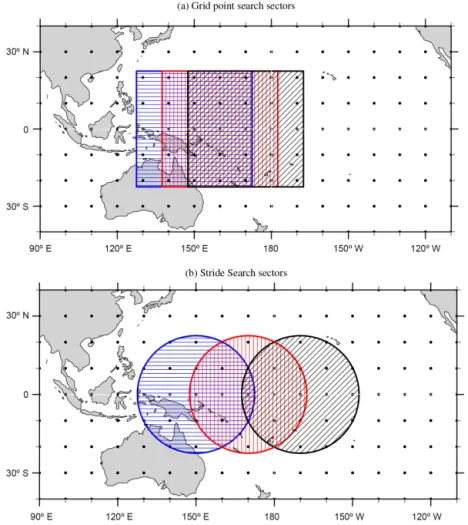
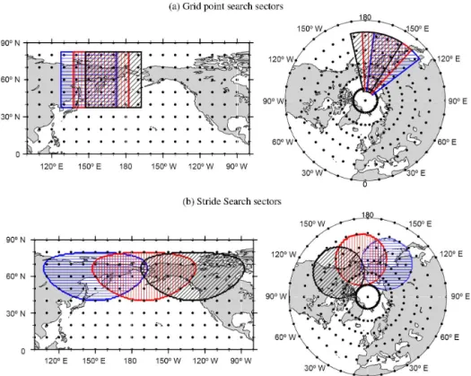
θmin andθmax can vary by application. Users must also se-lect a value fornthat relates the spatial scale of the storms they wish to detect to the resolution of the data1λ. Fig-ure 1a shows grid point search sectors along the equator withn=2 for data with resolution 1λ=10◦. The sectors
are 5×5 boxes in grid point space and span approximately 5600 km×5600 km on the Earth.
For each sector, the software collects data from the(2n+ 1)×(2n+1)points centered at(λj, θi). The collected data are compared against the storm identification criteria. If the cri-teria are met or exceeded in the sector, the algorithm checks if(λj, θi)is the location of the storm within that sector. If so, the algorithm records the storm to its output list. If not, the algorithm cycles to the next grid point, say(λj+1, θi), and begins again. In Fig. 1a the blue, horizontally striped sector is centered at(λj, θi)=(150◦E, 0◦N) and the next two con-secutive sectors are shown by the red, vertically striped sector centered at(λj+1, θi)=(160◦E, 0◦N) and black, diagonally striped sector whose center is(λj+2, θi)=(170◦E, 0◦N).
Centering a sector at each grid point in the search domain yields a robust algorithm. It ensures that the entire search do-main will be covered and that the same storm will not be recorded twice. Even though a single storm may trigger the identification criteria in several sectors, only the sector whose center corresponds to the storm location will be recorded to output. While the robustness of the grid point search algo-rithm is an advantage, it comes at the cost of redundant work. The same data points are accessed multiple times because the algorithm only advances one grid point at a time and the overlap of adjacent sectors is considerable.
The data access required by a grid point search and the overlap of adjacent sectors is also illustrated by Fig. 1a. All three sectors read the data from grid points in the re-gion{(λ, θ ): 150◦E≤λ≤170◦E, 20◦S≤θ≤20◦N}. For
visual clarity we have not plotted the sectors at(λj−1, θi)or (λj, θi±1), which would also overlap a majority of the same grid points.
2.2 Stride Search
Instead of squares in grid point space, Stride Search sectors are circles on the surface of an Earth-sized sphere. The sec-tors are defined using the geodesic distance function distG (λ1, θ1), (λ2, θ2)=
Figure 1.Adjacent search sectors along the equator. Black dots represent data points with resolution1λ=10◦. Blue sector (horizontal striping) center isλ=150◦E,θ=0◦N. Red (vertical striping) and black (diagonal striping) sectors are the next two consecutive searches;
(a)grid point search,n=2;(b)Stride Search,s=2220 km.
The numberSlat=s/adefines the arc length correspond-ing to the user-specified scales. We refer toSlatas the latitude stride and use it to define lines of constant latitude
θI=θmin+SlatI, I=0, . . ., Nθ, (4) whereNθ= ⌊(θmax−θmin)/Slat⌋ +1. The setθI divides the search domain into latitudinal strips of width≈s. We also define a longitude stride for eachθI,
Slon(I )=min
s acosθI
,2π
, I =0, . . ., Nθ, (5)
so that S(I )lonare the arc lengths along each latitude circle θI that approximately span a geodesic distance sin the longi-tudinal (zonal) direction. The minimum function in Eq. (5) accounts for the case where θI is either pole. The longi-tude stride defines points λI J along each latitude line θI, whereJ=(j−1)Slon(I )for j=1, . . ., Nλ(I ), creatingNλ(I )= ⌊2π/Slon(I )⌋longitude points along eachθI.
Each point (λI J, θI) defines the center of search sector KI J, whereKI J is the set of all points on the sphere lying
within a distancesof(λI J, θI),
KI J =(λ, θ ):distG (λ, θ ), (λI J, θI)≤s . (6) We note that the definition of the Stride Search sectors is determined entirely by the application-related spatial scales
and is therefore independent of resolution of the data,1λ.
By construction, sectorKI J overlaps its neighborsKI±1,J andKI,J±1by approximately one radiussin physical space. This is a sufficient condition to ensure that the entire search domain will be covered by the circular search sectors.
Figure 1b shows three consecutive circular sectors with
s=2220 km. This value ofs corresponds to an arc length of ≈20◦, and was chosen to match the scale of the sec-tors in Fig. 1a. The blue, horizontally striped circle is cen-tered at(λI J, θI)=(150◦E, 0◦N). The red, vertically striped sector is centered at (λI,J+1, θI)=(170◦E, 0◦N) and the center of the black, diagonally striped sector is located at
982 hPa
988 hPa 984 hPa
s
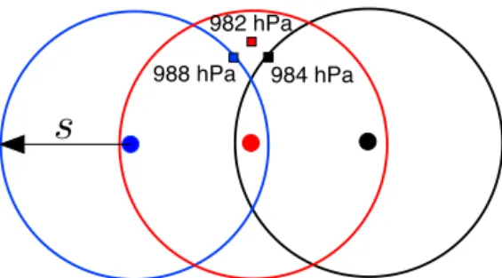
Figure 2. Duplicate detections of the same storm using the Stride Search algorithm. Each sector (blue/left, red/middle, and black/right) locates its minimum sea-level pressure (corresponding squares). Duplicate entries are removed prior to the output stage; only the red 982 hPa entry will remain.
Stride Search algorithm therefore covers a much larger geo-graphic area with the same number of search sectors.
Stride Search setup is completed by defining the sectors
KI J in terms the available data. Computationally, this in-volves creating a class and/or methods that identify and link each sector to the data points enclosed by its geographic boundary. Sectors used with high-resolution data sets auto-matically link to more grid points than the same-sized sec-tors used with lower-resolution data. For uniform longitude– latitude grids, Eq. (1) applies and the process is straightfor-ward. For unstructured grids, the mesh’s connectivity infor-mation may include a node adjacency list or topological data structures such as edges and faces. Any of these may be used to determine a sector’s enclosed data points. In the absence of such connectivity information, akd-tree algorithm (e.g., Samet, 2006) may be used.
Reduced overlap between adjacent sectors leads to im-proved performance by decreasing the number of redun-dant data accesses and by reducing the total number of tors. However, it also creates a new issue. Since each sec-tor is searched independently, several secsec-tors may detect and record the same storm to the linked list, as illustrated by Fig. 2. Before the storms detected by Stride Search can be saved to output, duplicate entries must be removed.
Duplicates are removed by again referencing the user-specified scale s. Each pair of entries in the linked list is compared; if a pair is separated by a distance less thans, the entries are considered duplicates and the less intense entry is deleted. In Fig. 2, this is demonstrated with pressure data. Each of the three search sectors have exceeded the storm identification criteria and independently locate their mini-mum pressure. The blue (left) sector finds a minimini-mum of 988 hPa, the red (middle) finds 982 hPa, and the black (right) finds 984 hPa. These three entries are clearly separated by a distance less thans, as they are all contained within the red (middle) circle. The duplicate removal procedure will delete the blue (left) and black (right) entries because, compared to the red (middle) entry, they have higher pressures and are less intense. Only the red 982 hPa entry will be saved to output.
In general, the list of detected storms at a particular time step, duplicates included, is much smaller than the spatial size of the data and the time required by the duplicate removal pro-cedure is negligible.
3 Data description
To demonstrate and test Stride Search we use data produced by the spectral element dynamical core of the Community Atmosphere Model, CAM-SE (Neale et al., 2012; Dennis et al., 2012). The model uses a cubed sphere grid and high-resolution experiments set 240 elements per face of the cube for a total of 3 110 402 horizontal grid points. This results in a horizontal resolution of 1λ≈0.125◦ (Worley et al.,
2011; Dennis et al., 2012). Due to well-known issues regard-ing the tunregard-ing of physical parameterizations within climate models, this resolution simulation may produce high-intensity storms with unrealistically high frequencies (Reed and Jablonowski, 2011; Dennis et al., 2012).
The original goals of the high-resolution experiments of Worley et al. (2011) and Dennis et al. (2012) were to demonstrate the parallel scaling of CAM-SE, to document its required run time and related statistics in various high-performance computing environments, and to demonstrate the model’s capability to produce well-resolved features like tropical cyclones that cannot be represented well in low-resolution experiments. Here, we choose these data because their high resolution ensures that small-scale storms will ex-ist, which provides a good testing environment for storm de-tection algorithms. The fact that there may be an unrealisti-cally high number of storms in the data is a benefit in this case.
The data set contains 5 years of simulated data that used CAM5 physics and preindustrial (year 1850) initial condi-tions. Instead of additional model components, the CAM-SE atmospheric dynamical core is coupled to a set of land, ocean, and sea ice data that also correspond to the year 1850 to provide its boundary conditions (Dennis et al., 2012). The land, ocean, and sea ice boundary conditions are periodic, with a period of 1 year, and simply repeat throughout the 5-year atmospheric simulation.
The model’s native cubed sphere data were interpolated to a uniform latitude–longitude grid with nlon=1024 for a resolution of 1λ=0.35◦ using the regridding software
provided by the Earth System Modeling Framework (Bal-aji et al., 2014). To facilitate a timing experiment (presented in the next section), we also interpolate 3 months of data to resolutions of1λ=2, 1, 0.5, and 0.25◦.
4 Tropical cyclones
which has a proven record. We also discuss the subtle dif-ferences between the two algorithms that lead to difdif-ferences in their final results that may be of importance to climate re-searchers.
While there are many different combinations of variables available to define a tropical cyclone (Walsh et al., 2007; Horn et al., 2014), to provide both codes with a common set of identification criteria we choose the TSTORMS default. A tropical cyclone is identified within search sector Kij if the following four criteria are met (Vitart et al., 1997):
1. There is a cyclonic vorticity maximum greater than a threshold value,τζ:
max i,j∈Kij
sgn(θi)·ζ850(λj, θi)> τζ, (7) whereζ850is the relative vorticity at the 850 hPa level. 2. The distance between the cyclonic vorticity maximum
and the sector’s sea-level pressure minimum is less than a threshold valueτD1 :
dist (λζ, θζ), (λP, θP)< τD1, (8)
where(λζ, θζ)and(λP, θP)are the locations of sector Kij’s vorticity maximum and sea-level pressure mini-mum, respectively.
3. The difference between the vertically averaged temper-ature’s maximum value and its sector average exceeds a thresholdτT:
max i,j∈Kij
T (λj, θi)−AvgKij(T ) > τT, (9)
whereT is defined as
T (λ, θ )=1
2 T500(λ, θ )+T200(λ, θ )
, (10)
and T500 and T200 are the temperatures at the 500 and 200 hPa pressure levels, respectively. To maintain consistency between both codes, the sector average AvgK
ij(T )is approximated as a simple arithmetic av-erage,
AvgKij(T )= 1
NKij X
{T (λj, θi):(λj, θi)∈Kij}, (11) whereNKij is the number of data points in sectorKij. 4. The distance between the maximum vertically averaged
temperature and the sea-level pressure minimum is less than a threshold valueτD2:
dist (λT, θT), (λP, θP)< τD2, (12)
where(λT, θT)is the location of the sector maximum of T.
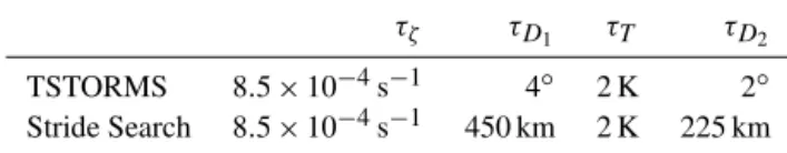
Table 1.Threshold values used for tropical cyclone detection.
τζ τD1 τT τD2
TSTORMS 8.5×10⁻⁴s−1 4◦ 2 K 2◦ Stride Search 8.5×10⁻⁴s−1 450 km 2 K 225 km
Differences between the two algorithms’ detections arise due to the differences in the algorithms themselves. For com-puting the collocation criteria, Eqs. (8) and (12), TSTORMS uses the angular distance function
distA (λ1, θ1), (λ2, θ2)= p
(λ2−λ1)2+(θ2−θ1)2. (13) For TSTORMS, whose intended application is in tropical re-gions, this is a simple and effective strategy because angu-lar distance is a reasonable proxy for geodesic distance near the equator. Stride Search uses the geodesic distance func-tion Eq. (3). Users of TSTORMS must specifyτD1 andτD2
in angular units, while users of Stride Search must use units of length. The arithmetic averages of the vertically averaged temperature Eq. (11) will be different from one algorithm to the other, because their sectors will contain a different num-ber of data points. As a result criteria 2, 3, and 4 may behave differently for each algorithm.
4.1 Spatial search results
We apply both algorithms to the data described in Sect. 3. We set TSTORMS n=12, Stride Search s=450 km, and use the threshold values shown in Table 1 for Eqs. (7), (8), (9), and (12).
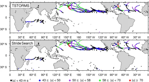
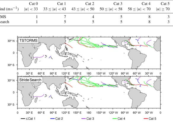
Results from an arbitrarily chosen 3 months of data, 18 July to 18 October of simulation year 4, are plotted in Fig. 3. Each dot represents a storm detected at one time step. All 6-hourly time steps over the entire 3 months are shown, colored by the windspeed-dependent hurricane categories de-fined by the Saffir–Simpson intensity scale.
Both algorithms produce qualitatively similar results. Vi-sually they appear to agree nearly perfectly on the identifi-able storm tracks and intensities. They both have false pos-itives over land and in the Southern Ocean. Stride Search produces more false positives, particularly in the Southern Ocean, than TSTORMS. This is due to the fact that Stride Search sectors – especially at higher latitudes – typically con-tain more data points than TSTORMS sectors. The larger number of points per sector reduces the sector average of the vertically averaged temperature, Eq. (11), compared to a TSTORMS sector at the same location. Thus, the warm core temperature excess criterion Eq. (9) is more easily achieved using Stride Search than TSTORMS for the same value of
Figure 3.Spatial search results, Northern Hemisphere summer simulation year 4. Each dot is a storm detected at one time step; colors correspond to the categories of the Saffir–Simpson hurricane scale.
of Eq. (9) between the codes will propagate into the storm tracks and final output.
4.2 Temporal correlation results
In this section we apply the temporal correlation algorithm, Algorithm 2, to the spatial search results. Since tropical cy-clones are inherently maritime events (Cotton and Anthes, 1989), at this stage we also apply a land mask to remove any tracks whose origins are not over water.
In Fig. 4 we show the storm tracks that correspond to the spatial search output of Fig. 3 with parameters Umax= 15 m s−1andtmin=2 days. These results show that the tem-poral correlation algorithm succeeds in eliminating false pos-itives and gives a better representation of the storms within the data set than the raw output from the spatial search rithm. Table 2 presents the final storm counts for each algo-rithm for the 3-month data set separated by hurricane cate-gory. Again, both algorithms produce nearly identical results which validate the present work.
Table 2 shows that Stride Search detects two fewer cat-egory 1 storms and one additional catcat-egory 2 storm than TSTORMS. Looking for differences between the panels of Fig. 4, we see that the category 1 storms correspond to a storm in the western Pacific off the east coast of Japan near (150◦E, 30◦W) and a storm in the north central Atlantic near
(050◦W, 20◦N).
Comparing the panels, we see that Stride Search classi-fied the western Pacific storm as category 2, which accounts for two of the three differences between rows in Table 2. Viewing the data, we note that the Stride Search track for this particular storm is 4 time steps longer than the corre-sponding TSTORMS track. During its final data points in the Stride Search output, the storm’s temperature excess was decreasing and very close to the detection threshold. Since
the TSTORMS sector average ofT is higher than the Stride Search sector average of T, the storm did not pass crite-rion 3 (Eq. 9) at the end of its life cycle in TSTORMS. We also find that this storm only achieved a category 2 wind speed at the very end of its life cycle, after the point in time where TSTORMS had stopped detecting it, which ex-plains why Stride Search counts the storm as a category 2 and TSTORMS does not.
A similar explanation holds for the Atlantic storm. We see that TSTORMS counts the same storm twice, once as a category 1 and once as a category 2, while Stride Search shows only one longer category 2 track. This is again due to the difference in the computation of the temperature ex-cess between the two codes. This particular storm weakened in its early days to the point where its temperature excess was not sufficient for TSTORMS to detect it before finally intensifying into a category 2 storm. This creates a hole in the TSTORMS track that does not show up in the Stride Search results because the temperature excess criterion is not as strict in Stride Search as it is in TSTORMS.
We point out that this is not a weakness of the TSTORMS software – our choice ofτT =2 K was somewhat arbitrary and choosing a lower threshold value τT for TSTORMS would remedy this problem for this particular cyclone. Rather, we stress that these differences arise simply due to the differences in the definition of both algorithms’ search sectors. To investigate these differences further we tested Stride Search using a midpoint rule quadrature approxima-tion of the sector average of the average vertical temperature, Eq. (11), and found similar results. We therefore chose to use the arithmetic average to keep the tropical cyclone identifica-tion criteria the same between the two codes.
Table 2.Storm count by hurricane category for Northern Hemisphere summer simulation year 4; this table corresponds to the storm tracks shown in Fig. 4.
Cat 0 Cat 1 Cat 2 Cat 3 Cat 4 Cat 5 Total
Max. wind (m s−1) |u|<33 33≤ |u|<43 43≤ |u|<50 50≤ |u|<58 58≤ |u|<70 |u| ≥70
TSTORMS 1 7 4 5 8 3 28
Stride Search 1 5 5 5 8 3 27
Figure 4.Storm tracks, Northern Hemisphere summer, simulation year 4. Each track is colored by the hurricane category corresponding to the maximum wind speed achieved during its lifetime.
size of the data set grows. Figure 5 shows the storm tracks produced by each algorithm for the entire data set, using the same identification criteria and threshold values as our previous discussion. Since the temperature excess criterion is more easily achieved by Stride Search, we would expect Stride Search to identify more storms than TSTORMS, par-ticularly in the lower-intensity storm categories. We might also expect TSTORMS to count too many storms because, for these threshold values, some storms may be split into multiple tracks. Both of these predictions may be born out in the data, which are tabulated in Table 3. Stride Search does indeed detect more category 0, 1, and 2 storms. TSTORMS also finds a higher number of high-intensity (category ≥3) storms than Stride Search, possibly due to track splitting. Without investigating differences in individual tracks, which is impractical for large data sets, one can only state that since the identification criteria used by both codes were identical, the different results can only be due to differences at the level of the algorithms’ design.
4.3 Performance and timing
As discussed previously, climate data sets are large and ex-pected to increase in size as climate models run at high reso-lutions with1λ <0.5◦. Storm detection algorithms must be
both accurate and efficient. In this section we document the
dependence of each search algorithm’s run time on the reso-lution of its input data set.
Differences in the structure of the two algorithms result in notable differences in the number of search sectors and the number of times each grid point is accessed in memory per time step. In the top row of Table 4 we present the total num-ber of search sectors required by each algorithm to search the tropical domain,θmin=40◦S,θ
max=40◦N for each data resolution. For TSTORMS this is equivalent to the number of grid points in the domain, hence the number of search sec-tors increases by a factor of 4 as the data resolution is halved. The number of Stride Search sectors remains constant across all data resolutions. For data on a uniform latitude–longitude grid, the number of points in a Stride Search sector grows as a function of latitude. The maximum points per sector listed for Stride Search are an upper bound that depends on the search domain, specificallyθminandθmaxand the spatial scales. For TSTORMS, the maximum points per sector are a function of the user-specified parameternand are equal to
(2n+1)×(2n+1).
sec-Table 3.Storm counts by hurricane category for the entire 5-year data set; this table corresponds to the storm tracks shown in Fig. 5.
Cat 0 Cat 1 Cat 2 Cat 3 Cat 4 Cat 5 Total
Max. wind (m s−1) |u|<33 33≤ |u|<43 43≤ |u|<50 50≤ |u|<58 58≤ |u|<70 |u| ≥70
TSTORMS 4 59 78 87 87 41 356
Stride Search 7 75 82 86 83 43 376
Figure 5.Storm tracks. The ultimate output of each algorithm for the entire 5-year data set. Coloring as in Fig. 4.
tors and reduced overlap between sectors in the Stride Search algorithm result in many fewer data accesses (by orders of magnitude) than the grid point search used by TSTORMS.
Both TSTORMS and the current implementation of Stride Search are written in Fortran and run in serial on a sin-gle thread. As a timing experiment, we run both codes on 3 months of data that were interpolated to resolutions of
1λ=2, 1, 0.5, and 0.25◦, as described in Sect. 3. Each
data set contains 360 time steps evenly spread across three NetCDF files. We chooses=450 km for Stride Search and set the TSTORMS parametern=2, 3, 6, 12 for the corre-sponding 1λ. The total wall clock time required for each algorithm to search each data set, including I/O, is recorded and the average time per time step is computed by dividing the total by 360. We repeat each experiment three times for each resolution and average the results to produce Fig. 6.
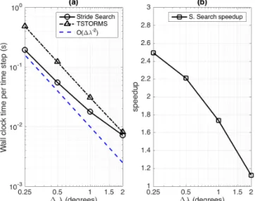
Figure 6a shows the average wall clock time required by each algorithm to search one time step of data as a function of the data resolution 1λ. The plot shows results from experiments run on a standard desktop workstation us-ing GNU’s Fortran compiler. The same tests were run on one node of Sandia’s Red Sky High Performance Comput-ing cluster usComput-ing the Intel Fortran compiler and produced similar results. Both algorithms appear to scale at the ex-pected rate ofO(1λ−2)as1λ→0, but for each resolution Stride Search is faster. The speed advantage of Stride Search over TSTORMS improves as resolution increases. Figure 6b
Figure 6.Timing results.(a)Average wall clock time required to search one time step of data.(b)Speedup due to Stride Search.
shows the speedup due to Stride Search, defined as the ra-tio of the TSTORMS average wall clock time per data time step to the Stride Search average wall clock time per data time step. Stride Search is approximately 15 % faster for the1λ=2◦data and this ratio increases as1λ→0. Stride
Table 4.Numbers of sectors, maximum data points per sector, and total number of data accesses per time step to search tropical domain
θ∈[40◦S, 40◦N] vs. data resolution. TSTORMS usedn= {2,3,6,12}for the corresponding1λ, and Stride Search useds=450 km.
TSTORMS Stride Search
1λ 2◦ 1◦ 0.5◦ 0.25◦ 2◦ 1◦ 0.5◦ 0.25◦
Number of sectors 7.29×10³ 2.92×10⁴ 1.17×10⁵ 4.66×10⁵ 1616 1616 1616 1616
Max. points per sector 25 49 169 625 49 143 437 1575
Max. data accesses 1.82×10⁵ 1.43×10⁶ 1.97×10⁷ 2.92×10⁸ 7.91×10⁴ 2.31×10⁵ 7.06×10⁵ 2.55×10⁶
Figure 7.Search sectors along 60◦N. Black dots represent data points with resolution1λ=10◦. Blue sector center isλ=150◦E,θ=60◦N.
Red and black sectors are the next two consecutive searches;(a)TSTORMS,n=2;(b)Stride Search,s=2500 km.
5 Polar search
A key motivation for developing Stride Search was to pro-vide a detection algorithm capable of searching all latitudes, including polar regions. The Arctic and Antarctic climates become increasingly frequent subjects of study due to re-cent significant changes in these environments (Stocker et al., 2013), and a detection algorithm capable of searching data near the poles is necessary. Grid point searches have been used at midlatitudes up to ≈60◦N and 60◦S (König et al.,
1993; Raible and Blender, 2004), but users must exercise care when choosing the sector size parameternat high lat-itudes. A grid point search near the poles may have to use sectors whose physical size is no longer representative of the physical features of the storms it is meant to locate.
Figure 7a shows three consecutive grid point search sec-tors along θ=60◦N. As in Fig. 1, the grid of data points
has resolution1λ=10◦and we have used the samen=2 to set up 5×5 grid point search sectors. The blue (horizontal stripes) sector is centered at (λj, θi)=(150◦E, 60◦N) and the red (vertical stripes) and black (diagonal stripes) sectors are at(λj+1, θi)=(160◦E, 60◦N) and(λj+2, θi)=(170◦E, 60◦N), respectively. Each grid point search sector spans
a distance of 5 grid points in latitude, or approximately 5600 km south to north.
The square grid point search sectors may appear correct in the left plot of Fig. 7a, a Mercator projection, but the problem with them is clear in the polar stereographic projection to the right. The southern boundary of each sector lies along the 40◦N latitude circle, where 5 grid points in longitude span
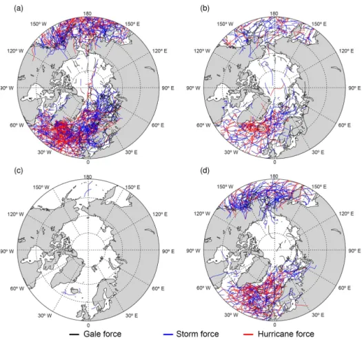
Figure 8.Northern Hemisphere polar low storm tracks by season;(a)DJF,(b)MAM,(c)JJA,(d)SON. Tracks are colored by the NOAA warning category corresponding to their lifetime maximum wind speed.
each sector, along 80◦N, spans only about 1000 km east to west. Users can choose higher values ofnat higher latitudes to ensure the sectors will have sufficient zonal extent to cap-ture the desired feacap-ture, but the square sectors will still have different spatial scales in the longitude direction compared to the latitude direction. As we have seen already in Sect. 4, the definition of search sector size can impact the final out-put of a search algorithm, independently of the identification criteria.
The constant geodesic radius of Stride Search sec-tors removes this dependence on the data. Figure 7b shows three Stride Search sectors along θ=60◦N, with
s=2500 km. The blue (horizontally striped) sector is centered at (λJ, θI)=(150◦E, 60◦N). The red (verti-cally striped) and black (diagonally striped) sectors are at (λj+1, θi)=(170◦W, 60◦N) and (λj+2, θi)=(130◦W, 60◦N), respectively. The longitude stride alongθ=60◦N is twice as large as the longitude stride along the equator, so the three consecutive sectors in Fig. 7b cover twice as many lon-gitude lines than the three sectors in Fig. 1b. The shapes of each sector in the left plot are due to the effects of the Mer-cator projection. All sectors are still circles on the sphere, as shown in the polar stereographic projection (right). Stride
Search sectors – even one centered at the pole – have the same geographic size regardless of latitude, and are therefore capable of searching polar regions as effectively as midlati-tude and tropical regions.
As an example application, we consider polar lows. Polar lows are distinct from midlatitude low-pressure systems due to their different developmental forcing and a typical lack of associated fronts (Montgomery and Farrell, 1992; Ras-mussen and Turner, 2003). They contribute to the break up of sea ice which has significant implications for the polar cli-mate.
A set of objective identification criteria for polar lows are given by Bracegirdle and Gray (2008), which we adapt to the Stride Search algorithm. Storm intensity is measured with vorticity and pressure and, as was the case with the tropi-cal cyclone identification criteria, a collocation requirement is applied. New to this application is a criterion that identi-fies regions of increased instability associated with cold air outbreaks over relatively warm ocean water.
Stride Search records a polar low in sectorKij if the fol-lowing criteria are met:
1. A sea-level pressure minimum of sufficient intensity ex-ists,
min i,j∈Kij
Psl(λj, θi) < τP, (14)
wherePsl is sea-level pressure andτP is the pressure threshold.
2. A cold air outbreak exists, min
i,j∈Kij
θ700(λj, θi)−SST(λj, θi)≤τT, (15)
whereθ700 is the potential temperature at the 700 hPa level, SST is the sea surface temperature, andτT is the cold air outbreak threshold.
3. A cyclonic vorticity maximum of sufficient strength ex-ists,
max i,j∈Kij
sgn(θi)ζ (λj, θi)> τζ. (16)
4. The vorticity maximum must be collocated with the pressure minimum,
dist (λP, θP), (λζ, θζ)< τD. (17) Stride Search setup uses a sector radius s=500 km, and search region boundaries θmin=45◦N, and θmax=90◦N. Threshold values are set at τP =980 hPa, τT =7 K, τζ= 2.0×10⁻⁴s−1 andτ
D=200 km. To the temporal correla-tion algorithm we add a minimum duracorrela-tion tmin=12 h and setUmax=20 m s−1.
The data include only temperature (not potential tempera-ture) and do not include the 700 hPa pressure level. The re-quiredθ700data are approximated as
θ700= 1
2(θ850+θ500) , (18)
whereθ850=T850
1000 850
0.286
andθ500=T500
1000 500
0.286 . Results from the entire 5-year data set are presented in Fig. 8, separated by season. Storm tracks are colored by their maximum strength on the US National Weather Ser-vice’s maritime warning scale (Bowditch, 2002); gale force
Figure 9.An example polar low on 25 December, simulation year 3, located at (017.0◦E, 86.5◦N) with structural similarities to a tropi-cal cyclone. The center of the plot is the North Pole and the perime-ter is the 80◦N latitude circle.
storms (black) have maximum wind speeds 17.5≤umax< 24.5 m s−1, storm force (blue) has 24.5≤u
max<33 m s−1, and hurricane force storms (red) have maximum wind speeds greater than 33 m s−1. The results show the expected seasonal variation of storm frequencies, with the maximum number of storms and the maximum intensity of storms occurring in the winter (DJF) months. Spring (MAM) months show more ac-tivity over the pole than the fall (SON) months, and there are few storms in the summer (JJA).
Once storm tracks are built, users may investigate indi-vidual storms more easily. To fulfill our goal of finding a “hurricane-like” polar low near the pole we search the storm tracks for storms that get within 5◦of the pole, then plot the
vorticity associated with each storm. Since the size of the storm track list is much smaller than the size of the data set, we quickly find the polar low shown in Fig. 9, from 12:00 UTC 25 December, simulation year 3. At the plotted time step the storm is located at (017.0◦E, 86.5◦N).
6 Conclusions
We have introduced the Stride Search algorithm for detection of extreme events within climate data sets. The algorithm is defined independently of a data set’s layout and resolution, and depends only on the spatial scale associated with a user’s intended application. Stride Search was designed to be a flex-ible algorithm, capable of searching data sets for a variety of extreme events while treating physical space the same for different data sets. Extreme events must be described by a set of quantifiable identification criteria and a representative spatial scale. As examples we have shown detections of two different varieties of cyclonic storms: tropical cyclones and polar lows. The capability to search polar latitudes in exactly the same manner as tropical and midlatitudes is a new feature introduced by Stride Search, and was the primary motivation for its development.
To validate Stride Search we compare its output to the output of TSTORMS, the current standard tool for tropi-cal cyclone detection. We show that Stride Search performs faster than TSTORMS and its relative speed up increases as the data resolution increases. The final outputs of both algo-rithms and tropical cyclone tracks, generally agree. However, due to their different definitions of spatial search sectors, re-sults between the two codes can differ in some cases even when both use the same identification criteria and threshold values.
Our results show that the storm track statistics associated with a particular climate data set can depend not only on the storm identification criteria, as is widely reported in the liter-ature (e.g., Bracegirdle and Gray, 2008; Raible et al., 2008; Horn et al., 2014), but also on the spatial search algorithm used to produce the storm tracks. Since the Stride Search al-gorithm is defined independently of data layout and resolu-tion, we posit that it may provide a more objective analysis tool and be less sensitive to differences in spatial discretiza-tions between data sets. Further experiments are necessary to investigate this claim; they should include variable resolution data, data defined on different types of spherical meshes, and sensitivity analyses covering a range of identification criteria and threshold values.
We anticipate that extending Stride Search to other, more specialized applications such as locating multicentered cy-clones (Hanley and Caballero, 2012) and atmospheric rivers (Ralph et al., 2004; Prabhat et al., 2012) will be straightfor-ward. The software uses the object-oriented design capabili-ties provided by modern Fortran (Adams et al., 2009) and is intended to allow users to extend its data types to new appli-cations.
Finally, we note that the performance of both Stride Search and TSTORMS software may be improved via paralleliza-tion. It is already common to take advantage of temporal par-allelism by applying the spatial search algorithm to multi-ple time steps and multimulti-ple files concurrently using several compute nodes. This may be implemented with customized
run scripts or dedicated software such as NASA’s Portable Distributed Script (PoDS) software (Kouatchou and Oloso, 2014), GNU Parallel (Tange, 2011), and the Toolkit for Ex-treme Climate Analysis (Prabhat et al., 2012). However, there also remains a significant amount of unexploited par-allelism in the storm detection problem, as individual search sectors at the same time step may be distributed across intra-node threads. We mark the parallel development of the Stride Search software as an additional item for future work. Code availability
A basic implementation of Stride Search written in Fortran for data on uniform latitude–longitude grids is available at https://github.com/pbosler/StrideSearch. The code is avail-able as open source and distributed under the GPL-2.0 li-cense. Development of a C++ implementation and support for unstructured grids are ongoing projects.
Acknowledgements. This work was supported by Sandia National Laboratories’ John von Neumann Postdoctoral Fellowship and by the Water Cycle and Climate Extremes Modeling project which is supported by the Office of Biological and Environmental Research in the DOE Office of Science. This research used resources of the Argonne Leadership Computing Facility at Argonne National Lab-oratory, which is supported by the Office of Science of the US De-partment of Energy under contract DE-AC02-06CH11357.
The authors thank GFDL and the creators of TSTORMS for pro-viding and maintaining this publicly available software. The authors also thank the referees, whose comments helped improve the article. Sandia National Laboratories is a multiprogram laboratory managed and operated by Sandia Corporation, a wholly owned subsidiary of Lockheed Martin Corporation, for the U.S. Depart-ment of Energy’s National Nuclear Security Administration under contract DE-AC04-94AL85000. SAND NO. 2015-4839J.
Edited by: A. Kerkweg
References
Adams, J. C., Brainerd, W. S., Hendrickson, R. A., Maine, R. E., Martin, J. T., and Smith, B. T.: The Fortran 2003 Handbook, Springer, 2009.
Bowditch, N.: The American Practical Navigator, Pub. No. 9, Na-tional Imagery and Mapping Agency, bicentennial Edn., avail-able at: http://www.nws.noaa.gov/om/marine/home.htm (last ac-cess: 7 July 2015), 2002.
Bracegirdle, T. J. and Gray, S. L.: An objective climatology of the dynamical forcing of polar lows in the Nordic seas, Int. J. Clima-tol., 28, 1903–1919, 2008.
Cotton, W. R. and Anthes, R. A.: Storm and Cloud Dynamics, Aca-demic Press, 1989.
Dennis, J. M., Edwards, J., Evans, K. J., Guba, O., Lauritzen, P. H., Mirin, A. A., St-Cyr, A., Taylor, M. A., and Worley, P. H.: CAM-SE: A scalable spectral element dynamical core for the Com-munity Atmosphere Model, Int. J. High Perform. C., 26, 74–89, 2012.
Føre, I., Kristjánsson, J. E., Kolstad, E. W., Bracegirdle, T. J., Sae-tra, Ø., and Røsting, B.: A “hurricane-like” polar low fuelled by sensible heat flux: High-resolution numerical simulations, Q. J. Roy. Meteor. Soc., 138, 1308–1324, 2012.
Geng, Q. and Sugi, M.: Variability of the North Atlantic cyclone activity in winter analyzed from NCEP-NCAR reanalysis data, J. Climate, 14, 3863–3873, 2001.
Hanley, J. and Caballero, R.: Objective identification and tracking of multicentre cyclones in the ERA-Interim reanalysis dataset, Q. J. Roy. Meteor. Soc., 138, 612–625, 2012.
Hodges, K. I.: A general method for tracking analysis and its ap-plication to meteorological data, Mon. Weather Rev., 122, 2573– 2586, 1994.
Horn, M., Walsh, K., Zhao, M., Camargo, S. J., Scoccimarro, E., Murakami, H., Wang, H., Ballinger, A., Kumar, A., Shaevitz, D. A., Jonas, J. A., and Oouchi, K.: Tracking scheme dependence of simulated tropical cyclone response to idealized climate sim-ulations, J. Climate, 27, 9197–9213, 2014.
Kleppek, S., Muccione, V., Raible, C. C., Bresch, D. N., Koellner-Heck, P., and Stocker, T. F.: Tropical cyclones in ERA-40: A de-tection and tracking method, Geophys. Res. Lett., 35, L10705, doi:10.1029/2008GL033880, 2008.
Knutson, T. R., Sirutis, J. J., Garner, S. T., Vecchi, G. A., and Held, I. M.: Simulated reduction in Atlantic hurricane frequency under twenty-first-century warming conditions, Nat. Geosci., 1, 359– 364, 2008.
König, W., Sausen, R., and Sielmann, F.: Objective identification of cyclones in GCM simulations, J. Climate, 6, 2217–2231, 1993. Kouatchou, J. and Oloso, A.: Portable Distributed Script (PoDS),
Tech. Rep. GSC-16531-1, NASA, 2014.
Montgomery, M. T. and Farrell, B. F.: Polar low dynamics, J. At-mos. Sci., 49, 2484–2505, 1992.
Neale, R., Chen, C., Gettlelman, A., Lauritzen, P. H., Park, S., Williamson, D. L., Conley, A. J., Garcia, R., Kinnison, D., Lamarque, J., Marsh, D., Mills, M., Smith, A. K., Tilmes, S., Vitt, F., Morrison, H., Cameron-Smith, P., Collins, W. D., Iacono, M. J., Easter, R. C., Ghan, S. J., Liu, X., Rasch, P. J., and Taylor, M. A.: Description of the NCAR Community Atmosphere Model (CAM 5.0), Tech. Rep. NCAR/TN-486+STR, NCAR, 2012. Neu, U., Akperov, M. G., Bellenbaum, N., Benestad, R., Blender,
R., Caballero, R., Cocozza, A., Dacre, H. F., Feng, Y., Fraedrich, K., Grieger, J., Gulev, S., Hanley, J., Hewson, T., Inatsu, M., Keay, K., Kew, S. F., Kindem, I., Leckebusch, G. C., Liberato, M. L. R., Lionello, P., Mokhov, I. I., Pinto, J. G., Raible, C. C., Reale, M., Rudeva, I., Schuster, M., Simmonds, I., Sinclair, M.,
Sprenger, M., Tilinina, N. D., Trigo, I. F., Ulbrich, S., Ulbrich, U., Wang, X. L., and Wernli, H.: IMILAST: A community ef-fort to intercompare extratropical cyclone detection and tracking algorithms, B. Am. Meterol. Soc., 94, 529–547, 2013.
Nordeng, T. E. and Rasmussen, E. A.: A most beautiful polar low. A case study of a polar low development in the Bear Island region, Tellus A, 44, 81–99, 1992.
Prabhat, U. O., Byna, S., Wu, K., Li, F., Wehner, M., and Bethel, E. W.: TECA: A Parallel Toolkit for Extreme Climate Analy-sis, in: Third Workshop on Data Mining in Earth System Sci-ence (DMESS 2012), LBNL-5352E, International ConferSci-ence on Computational Science (ICCS 2012), available at: http://vis.lbl. gov/Vignettes/2012-climatePatterns-vignette/ (last access: 6 Jan-uary 2015), Omaha NE, 2012.
Putnam, W. M. and Lin, S.-J.: Finite-volume transport on various cubed-sphere grids, J. Comput. Phys., 227, 55–78, 2007. Raible, C. C. and Blender, R.: Northern hemisphere midlatitude
cy-clone variability in GCM simulations with different ocean repre-sentations, Clim. Dynam., 22, 239–248, 2004.
Raible, C. C., Della-Marta, P. M., Schwierz, C., Wernli, H., and Blender, R.: Northern hemisphere extratropical cyclones: A com-parison of detection and tracking methods and different reanaly-ses, Mon. Weather Rev., 136, 880–897, 2008.
Ralph, F. M., Nieman, P. J., and Wick, G. A.: Satellite and aircraft observations of atmospheric rivers over the eastern North Pacific ocean during the winter of 1997/98, Mon. Weather Rev., 132, 1721–1745, 2004.
Rasmussen, E. A. and Turner, J. (Eds.): Polar Lows: Mesoscale Weather Systems in the Polar Regions, Cambridge University Press, 2003.
Reed, K. A. and Jablonowski, C.: Assessing the uncertainty in tropical cyclone simulations in NCAR’s Community At-mosphere Model, J. Adv. Mod. Earth Sys., 3, M08002, doi:10.1029/2011MS000076, 2011.
Roesler, E. L., Bosler, P. A., and Taylor, M. A.: Arctic storms in a re-gionally refined atmospheric general circulation model, in prepa-ration, 2016.
Samet, H.: Foundations of Multidimensional and Metric Data Struc-tures, Morgan Kaufman, San Francisco CA, USA, 2006. Sinclair, M. R.: An objective cyclone climatology for the Southern
Hemisphere, Mon. Weather Rev., 122, 2239–2256, 1994. Sinclair, M. R.: Objective identification of cyclones and their
cir-culation intensity, and climatology, Weather Forecast., 12, 595– 612, 1997.
Skamarock, W. C., Klemp, J. B., Duda, M. G., Fowler, L. D., and Park, S.-H.: A multiscale nonhydrostatic atmospheric model using centroidal Voronoi tesselations and C-grid staggering, Mon. Weather Rev., 140, 3090–3105, doi:10.1175/MWR-D-11-00215.1, 2012.
Assess-ment Report of the IntergovernAssess-mental Panel on Climate Change, Tech. rep., IPCC, 2013.
Tange, O.: GNU Parallel – The command-line power tool, The USENIX Magazine, 36, 42–47, 2011.
TSTORMS: Diagnosis and Detection of Tropical Storms in High-Resolution Atmospheric Models, available at: http://www.gfdl. noaa.gov/tstorms (last access: 27 January 2015), 1997.
Vitart, F. and Stockdale, T. N.: Seasonal forecasting of tropical storms using coupled GCM integrations, Mon. Weather Rev., 129, 2521–2537, 2001.
Vitart, F., Anderson, J. L., and Stern, W. F.: Simulation of inter-annual variability of tropical storm frequency in an ensemble of GCM integrations, J. Climate, 10, 745–760, 1997.
Walsh, K. J. E., Fiorino, M., Landsea, C. W., and McInnes, K. L.: Objectively determined resolution-dependent threshold criteria for the detection of tropical cyclones and reanalyses, J. Climate, 20, 2307–2314, 2007.
Wernli, H. and Schwierz, C.: Surface cyclones in the ERA-40 dataset (1958–2001). Part I: Novel identification method and global climatology, J. Atmos. Sci., 63, 2486–2507, 2006.
Williamson, D. L.: Storm track representation and verification, Tel-lus, 33, 513–530, 1981.
Worley, P. H., Craig, A. P., Dennis, J. M., Mirin, A. A., Tay-lor, M. A., and Vertenstein, M.: Performance of the Com-munity Earth System Model, in: International Conference for High Performance Computing, Networking, Storage and Anal-ysis (SC11), 2011.
Zarzycki, C. M. and Jablonowski, C. J.: A multidecadal simulation of Atlantic tropical cyclones using a variable resolution global atmosphere general circulation model, J. Adv. Mod. Earth Sys., 6, 805–828, 2014.