The multi-scale aerosol-climate model PNNL-MMF: model description and evaluation

(1)

GMDD

3, 1625–1695, 2010

A multi-scale aerosol climate model

M. Wang et al.

Title Page

Abstract Introduction

Conclusions References

Tables Figures

◭ ◮

Back Close

Full Screen / Esc

Printer-friendly Version Interactive Discussion

Discussion

P

a

per

|

Dis

cussion

P

a

per

|

Discussion

P

a

per

|

Discussio

n

P

a

per

|

Geosci. Model Dev. Discuss., 3, 1625–1695, 2010 www.geosci-model-dev-discuss.net/3/1625/2010/ doi:10.5194/gmdd-3-1625-2010

Geoscientific Model Development Discussions

This discussion paper is/has been under review for the journal Geoscientific Model Development (GMD). Please refer to the corresponding final paper in GMD if available.

The multi-scale aerosol-climate model

PNNL-MMF: model description and

evaluation

M. Wang1, S. Ghan1, R. Easter1, M. Ovchinnikov1, X. Liu1, E. Kassianov1, Y. Qian1, W. Gustafson1, V. E. Larson2, D. P. Schanen2, M. Khairoutdinov3, and H. Morrison4

1

Atmospheric Science and Global Change Division, Pacific Northwest National Laboratory, Richland, Washington, USA

2

Department of Mathematical Sciences, University of Wisconsin – Milwaukee, Milwaukee, Wisconsin, USA

3

School of Marine and Atmospheric Sciences, Stony Brook University, Stony Brook, New York, USA

4

Mesoscale and Microscale Meteorology Division, National Center for Atmospheric Research, Boulder, Colorado, USA

Received: 18 September 2010 – Accepted: 21 September 2010 – Published: 8 October 2010

Correspondence to: M. Wang (minghuai.wang@pnl.gov)

(2)

GMDD

3, 1625–1695, 2010

M. Wang et al.

Title Page

Tables Figures

◭ ◮

Back Close

Full Screen / Esc

Discussion

P

a

per

|

Dis

cussion

P

a

per

|

Discussion

P

a

per

|

Discussio

n

P

a

per

|

Abstract

Anthropogenic aerosol e_ffects on climate produce one of the largest uncertainties in

estimates of radiative forcing of past and future climate change. Much of this uncer-tainty arises from the multi-scale nature of the interactions between aerosols, clouds

and large-scale dynamics, which are di_fficult to represent in conventional global

cli-5

mate models (GCMs). In this study, we develop a multi-scale aerosol climate model

that treats aerosols and clouds across different scales, and evaluate the model

per-formance, with a focus on aerosol treatment. This new model is an extension of a multi-scale modeling framework (MMF) model that embeds a cloud-resolving model

(CRM) within each grid column of a GCM. In this extension, the effects of clouds on

10

aerosols are treated by using an explicit-cloud parameterized-pollutant (ECPP) ap-proach that links aerosol and chemical processes on the large-scale grid with statistics of cloud properties and processes resolved by the CRM. A two-moment cloud mi-crophysics scheme replaces the simple bulk mimi-crophysics scheme in the CRM, and a modal aerosol treatment is included in the GCM. With these extensions, this

multi-15

scale aerosol-climate model allows the explicit simulation of aerosol and chemical pro-cesses in both stratiform and convective clouds on a global scale.

Simulated aerosol budgets in this new model are in the ranges of other model stud-ies. Simulated gas and aerosol concentrations are in reasonable agreement with ob-servations, although the model underestimates black carbon concentrations at the

sur-20

face. Simulated aerosol size distributions are in reasonable agreement with obser-vations in the marine boundary layer and in the free troposphere, while the model underestimates the accumulation mode number concentrations near the surface, and overestimates the accumulation number concentrations in the free troposphere. Sim-ulated cloud condensation nuclei (CCN) concentrations are within the observational

25

(3)

GMDD

3, 1625–1695, 2010

M. Wang et al.

Title Page

Tables Figures

◭ ◮

Back Close

Full Screen / Esc

Discussion

P

a

per

|

Dis

cussion

P

a

per

|

Discussion

P

a

per

|

Discussio

n

P

a

per

|

strong fossil fuel and biomass burning emissions, and overestimates AOD over regions with strong dust emissions. Overall, this multi-scale aerosol climate model simulates aerosol fields as well as conventional aerosol models.

1 Introduction

Atmospheric aerosols are an important component of the global climate system. They

5

can affect the climate system directly by scattering or absorbing solar radiation, and

indirectly through their effects on clouds by acting as cloud condensation nuclei (CCN)

or ice nuclei (IN). However, despite more than a decade of active research,

anthro-pogenic aerosol effects on climate still produce one of the largest uncertainties in the

estimates of radiative forcing of past and future climate change (IPCC, 2007).

10

Much of this uncertainty arises from the multi-scale nature of the interactions

be-tween aerosols, clouds and large-scale dynamics, which are difficult to represent in

conventional global climate models (GCMs). These interactions span a wide range in spatial scales, from 0.01–1000 µm for droplet and crystal nucleation, aqueous-phase chemistry, precipitation, and collection, to 100–1000 m for marine stratus, to 1–2 km

15

for shallow cumulus, to 2–10 km for deep convection, and to 50–100 km for large scale cloud systems. Given the typical GCM grid spacing of 100–400 km, the treatment of most of those processes in conventional GCMs is highly parameterized and, therefore, also highly uncertain.

Representing aerosol/cloud processes in deep cumulus has been most

problem-20

atic in global climate models. Cumulus parameterizations in current climate models rely on ad hoc closure assumptions designed to diagnose the latent heating and ver-tical transport of heat and moisture by deep convection, and provide little information about microphysics or updraft velocity (Del Genio et al., 2005; Emanuel and

Zivkovic-Rothman, 1999; Zhang et al., 2005). As a result, aerosol effects on cumulus clouds are

25

(4)

GMDD

3, 1625–1695, 2010

M. Wang et al.

Title Page

Tables Figures

◭ ◮

Back Close

Full Screen / Esc

Discussion

P

a

per

|

Dis

cussion

P

a

per

|

Discussion

P

a

per

|

Discussio

n

P

a

per

|

field and satellite measurements and simulations by cloud-resolving models (CRMs) provide increasing evidence that aerosols influence cumulus clouds (Andreae et al., 2004; Cui et al., 2006; Koren et al., 2004, 2005; Rosenfeld et al., 2008; Wang, 2005).

In addition, cumulus clouds play critical roles in determining the vertical distributions and lifetime of most aerosols. Convective clouds are responsible for much of the

ver-5

tical transport of pollutants, the aqueous chemistry, and the removal of pollutants from the atmosphere (Chatfield and Crutzen, 1984; Ekman et al., 2006; Wang and Prinn, 2000). Easter et al. (2004) showed that convective clouds account for 80–95% of accumulation-mode aerosol number removal, 65–85% of carbonaceous aerosol wet

removal, 50–85% of sulfate wet removal, and 10–70% of in-cloud SO₂ oxidation in

10

their global aerosol climate model. However, the treatment of convective cloud pro-cesses in global aerosol models is based on cumulus parameterizations, which are highly uncertain (Bechtold et al., 2000; Xie et al., 2002; Xu et al., 2002; Gregory and Guichard, 2002). In the global aerosol climate model used by Easter et al. (2004), the

large range (10–70%) for in-cloud SO₂ oxidation reflects di_fferent assumptions made

15

about the cloud volume of convective clouds, which is generally not predicted by cu-mulus parameterizations. Simulated vertical distributions of gas and aerosol species in global models have been shown to largely depend on the convective parameterization (Iversen and Seland, 2002; Jacob et al., 1997; Mahowald et al., 1995; Rasch et al., 2000).

20

To avoid the problems in cumulus parameterizations in GCMs, Suzuki et al. (2008) simulated aerosol-cloud interactions in convective clouds on global scale by using an aerosol-coupled global CRM with a horizontal grid spacing of 7 km. They showed that

the model realistically simulated detailed spatial structure of cloud droplet e_ffective

radii and the relationship between liquid water path and aerosol optical properties,

25

(5)

GMDD

3, 1625–1695, 2010

M. Wang et al.

Title Page

Tables Figures

◭ ◮

Back Close

Full Screen / Esc

Discussion

P

a

per

|

Dis

cussion

P

a

per

|

Discussion

P

a

per

|

Discussio

n

P

a

per

|

A new type of global climate model called the multi-scale modeling framework (MMF) model, first introduced a decade ago (Grabowski, 2001; Khairoutdinov and Randall, 2001), uses a cloud resolving model (CRM) at each grid column of a host GCM to replace conventional parameterizations for moist convection and large scale conden-sation. This approach permits explicit simulations of deep convective clouds for the

5

whole global domain, while keeping the computational cost acceptable for multi-year climate simulations. The subgrid variability in cloud dynamics and cloud microphysics is explicitly resolved at spatial scales down to the resolution of the CRM. The MMF models have been shown to improve climate simulations in several important ways (Ovtchinnikov et al., 2006; Pritchard and Somerville, 2009a, b; Khairoutdinov et al.,

10

2008; Tao et al., 2009).

The MMF model would be an ideal tool to study aerosol e_ffects on climate on global

scale given its multi-scale nature and its moderate computational cost compared with global CRMs. However, several limitations in the original MMF (Khairoutdinov et al.,

2008) have hindered its usage in studying aerosol e_ffects on climate. First, the

origi-15

nal MMF did not include any treatment of aerosol and chemical processes. Second, the original MMF has an oversimplified microphysics treatment consisting of only two predicted water variables. This simple scheme neglected the complex interactions

be-tween different hydrometers and did not represent a variety of processes (e.g., the

Bergeron-Findeisen process, droplet activation, and ice nucleation) that are important

20

to the study of aerosol-cloud interactions.

In this study, we address these challenges and extended the original MMF in the following ways. First, the host GCM model is updated to use a modal aerosol approach to treat aerosol processes and represent aerosol size distributions; second, an explicit-cloud parameterized-pollutant (ECPP) approach (Gustafson et al., 2008) is added to

25

(6)

GMDD

3, 1625–1695, 2010

M. Wang et al.

Title Page

Tables Figures

◭ ◮

Back Close

Full Screen / Esc

Discussion

P

a

per

|

Dis

cussion

P

a

per

|

Discussion

P

a

per

|

Discussio

n

P

a

per

|

aerosol-cloud interactions from cumulus to global scales. In this paper, we have docu-mented these changes, with a focus on aerosol and chemical treatment, and evaluate the model results. Section 2 documents the improvements in detail, and the model results are shown in Sects. 3 and 4. Finally, Sect. 5 is the summary.

2 Model description and set-up of simulations

5

The PNNL-MMF is an extension of the Colorado State University (CSU) MMF model (Khairoutdinov et al., 2005, 2008), first developed by Khairoutdinov and Randall (2001). The CSU MMF was based on the Community Atmospheric Model (CAM) version 3.5, which is the atmospheric component of the NCAR Community Climate System Model

(Collins et al., 2006). The embedded CRM in each GCM grid column is a

two-10

dimensional version of the System for Atmospheric Modeling (SAM) (Khairoutdinov and Randall, 2003), which replaces the conventional moist physics, convective, turbu-lence, and boundary layer parameterizations, except for the gravity wave drag param-eterization in CAM. During each GCM time step (every 10 min), the CRM is forced by the large-scale temperature and moisture tendencies arising from GCM-scale

dynami-15

cal process and feeds the response back to the GCM-scale as heating and moistening terms in the large-scale budget equations for heat and moisture. The CRM runs con-tinuously using a 20-s time step. The CAM radiative transfer code is applied to each CRM column at every GCM time step (10 min), assuming 1 or 0 cloud fraction at each CRM grid point, which eliminates the cloud overlap assumptions used in conventional

20

GCMs.

In this study, both the GCM and CRM components are updated from what is used in the CSU MMF. A third component, the ECPP approach, is added to link aerosol and chemical processes on the GCM grids with statistics of cloud properties resolved by the CRM. Those extensions in the PNNL-MMF are documented in detail below.

(7)

GMDD

3, 1625–1695, 2010

M. Wang et al.

Title Page

Tables Figures

◭ ◮

Back Close

Full Screen / Esc

Discussion

P

a

per

|

Dis

cussion

P

a

per

|

Discussion

P

a

per

|

Discussio

n

P

a

per

|

2.1 The NCAR CAM5 atmospheric GCM

The host GCM in the PNNL MMF has been updated to version five of CAM (CAM5).

Although CAM5 differs from CAM3.5 in many respects (e.g., cloud microphysics, cloud

macrophysics, turbulence, shallow cumulus, aerosols, and radiative transfer), most of the changes are not relevant to the MMF model since the treatments of clouds and

tur-5

bulence are replaced with the treatments in the CRM. The differences that are relevant

to the MMF model are in the treatment of radiative transfer and of the aerosol lifecycle, which are briefly described below.

The radiative transfer scheme in CAM5 is the Rapid Radiative Transfer Model for GCMs (RRTMG), a broadband k-distribution radiation model developed for application

10

to GCMs (Iacono et al., 2003, 2008; Mlawer et al., 1997).

A modal approach is used to treat aerosols in CAM5 (Liu et al., 2010). Aerosol size distributions are represented by using three or seven log-normal modes. The three-mode version adopted in this study has been shown to simulate aerosol fields in

rea-sonable agreement with the 7-mode treatment and is computationally more efficient,

15

which makes it more suitable for long-term climate simulations (Liu et al., 2010). The three-mode version has an Aitken mode, an accumulation mode, and a single coarse mode. Aitken mode species include sulfate, secondary organic carbon (SOA), and sea salt; accumulation mode species include sulfate, SOA, black carbon (BC), primary or-ganic carbon (POM), sea salt, and dust; coarse mode species include sulfate, sea salt,

20

and dust. Species mass and number mixing ratios are predicted for each mode, while mode widths are prescribed. Both aerosols outside the cloud droplets (interstitial) and aerosols in the cloud droplets (cloud-borne) are predicted. Aerosol nucleation from

H₂SO₄, condensation of trace gases (H₂SO₄, and semi-volatile organics) on existing

aerosol particles, and coagulation (Aitken and accumulation modes) are treated.

Wa-25

ter uptake and optical properties for each mode are expressed in terms of both relative humidity (accounting for hysteresis) and the hygroscopicities of the mode’s

(8)

GMDD

3, 1625–1695, 2010

M. Wang et al.

Title Page

Tables Figures

◭ ◮

Back Close

Full Screen / Esc

Discussion

P

a

per

|

Dis

cussion

P

a

per

|

Discussion

P

a

per

|

Discussio

n

P

a

per

|

averaged oxidant fields (OH, O₃, and NO₃) produced by a version of CAM with detailed

gas-phase chemistry.

In the standard CAM5, cloud fields from the conventional cloud parameterizations are used to drive the convective transport, aerosol activation in stratiform clouds, aque-ous chemistry, and wet scavenging for aerosol and gas species. In the PNNL-MMF, the

5

treatment of cloud-related aerosol and gas processes (i.e., aqueous chemistry, con-vective transport, and wet scavenging) in the standard CAM5 is replaced by the ECPP approach (Sect. 2.3), which uses cloud statistics simulated by the CRM to drive the aerosol processing by clouds.

2.2 The SAM CRM

10

The original SAM used in the CSU MMF had a simple bulk microphysics scheme in which only the liquid/ice-water moist static energy, the total nonprecipitating water, and the total precipitating water were predicted (Khairoutdinov and Randall, 2003). The mixing ratio of cloud water, cloud ice, rain, snow and graupel were diagnosed from the prognostic variables using temperature-dependent partitioning between liquid and ice.

15

This simple scheme neglected the complex interactions between different hydrometers

and was not able to represent a variety of processes (e.g., the Bergeron-Findeisen pro-cess, droplet activation, and ice nucleation) that are important to the study of aerosol-cloud interactions.

In the PNNL-MMF, a double-moment microphysics scheme from Morrison

20

et al. (2005, 2009) replaces the simple bulk microphysics in the CRM model. The new scheme predicts the number concentrations and mixing ratios of five hydrometer types (cloud droplets, ice crystals, rain, snow, and graupel). The precipitation hydrom-eter types (rain, snow, and graupel) are fully prognostic in the CRM model, rather than diagnostic as in CAM5. Droplet activation from hydrophilic aerosols, ice nucleation,

25

(9)

GMDD

3, 1625–1695, 2010

M. Wang et al.

Title Page

Tables Figures

◭ ◮

Back Close

Full Screen / Esc

Discussion

P

a

per

|

Dis

cussion

P

a

per

|

Discussion

P

a

per

|

Discussio

n

P

a

per

|

Droplet activations are calculated at each CRM grid point, based on the parameteri-zation of Abdul-Razzak and Ghan (2000). The vertical velocity used in droplet activa-tion is the sum of the vertical velocity resolved at the CRM grid point and a sub-grid

vertical velocity (σcrmw) that accounts for the unresolved motion. The subgrid vertical

velocity is diagnosed from the turbulent kinetic energy (TKE):σ_crmw=

q

(TKE/3), where

5

the TKE is predicted or diagnosed in the SAM CRM, depending on its sub-grid model. A simple Smagorinsky-type scheme is used to treat the subgrid-scale fluxes in the SAM model, and the TKE is diagnosed from the eddy viscosity. A minimum vertical velocity of 0.1 m s−1is set for calculating droplet activation. Aerosol fields used in droplet acti-vation in the CRM are predicted on the GCM grid cells by CAM5, in which cloud-related

10

aerosol processes are treated by using the ECPP approach (Sect. 2.3).

The CAM radiative transfer scheme (RRTMG) is applied to each CRM column, as-suming 1 or 0 cloud fraction at each CRM grid point. Aerosol water uptake is calculated at each CRM grid point, which accounts for the subgrid variation in relative humidity within each GCM grid cell. Aerosol water at the CRM grids together with dry aerosol

15

on the GCM grids are used to calculate aerosol optical properties at each CRM grid.

2.3 The Explicit-Cloud-Parameterized-Pollutant (ECPP) approach

As we discussed in the introduction, one of the limitations in the CSU MMF is its lack of treatment of aerosol and chemical processes. An ideal way to account for these pro-cesses in the MMF model would be to add their treatment into the CRM component,

20

thereby simulating aerosol and chemical processes directly on cloud scales. Given the large number of species and numerous processes involved, however, this approach is not computationally feasible for multi-year climate simulations in the near future. In this study, we take an alternative approach, the Explicit-Cloud Parameterized-Pollutant method (ECPP) (Gustafson et al., 2008). The ECPP approach uses statistics of cloud

25

(10)

GMDD

3, 1625–1695, 2010

M. Wang et al.

Title Page

Tables Figures

◭ ◮

Back Close

Full Screen / Esc

Discussion

P

a

per

|

Dis

cussion

P

a

per

|

Discussion

P

a

per

|

Discussio

n

P

a

per

|

account for the effects of convective clouds on aerosols while being computationally

feasible. The treatment of vertical transport of tracers within ECPP is documented in detail in Gustafson et al. (2008) and is slightly modified in this study. The ECPP treat-ment is also extended to treat aerosol activation, resuspension (cloud-borne aerosol particles are resuspended and become interstitial aerosol particles due to the

evapo-5

ration of cloud droplets), aqueous chemistry and wet scavenging.

In the ECPP approach, the aerosol species and aerosol precursor gases are carried on the CAM grid, while cloud variables are carried on the CRM grid. Large scale trans-port of the aerosol and gas tracers and several “non-cloud” processes (emissions, verti-cal turbulent mixing, dry deposition, gas-phase chemistry, condensation/evaporation of

10

gases on aerosols, aerosol nucleation, and aerosol coagulation) are calculated on the CAM grid. The resulting tracer distributions are passed to ECPP, in which information from the CRM is used to better simulate cloud processing of aerosols and trace species (i.e., vertical transport, aerosol activation/resuspension, aqueous chemistry, convective transport, and precipitation scavenging). The resulting aerosol fields from ECPP are

15

then used in the CRM for cloud microphysics (droplet nucleation) and aerosol optical property calculations.

Besides using cloud statistics from the CRM instead of those from the conventional cloud parameterizations in CAM5 to drive aerosol and chemical processing by clouds,

the ECPP approach differs from that in the conventional CAM5 in several other

impor-20

tant aspects. First, the ECPP approach predicts both interstitial aerosols and cloud-borne (in-cloud) aerosols in all clouds, while the conventional CAM5 does not treat cloud-borne aerosols in convective clouds. So the conventional CAM5 needs to as-sume a convective-cloud activation fraction for each mode, which is used in computing in-cloud scavenging. In the ECPP approach, the cloud-borne aerosols in convective

25

(11)

GMDD

3, 1625–1695, 2010

M. Wang et al.

Title Page

Tables Figures

◭ ◮

Back Close

Full Screen / Esc

Discussion

P

a

per

|

Dis

cussion

P

a

per

|

Discussion

P

a

per

|

Discussio

n

P

a

per

|

process-split approach to treat convective transport, wet scavenging and aqueous chemistry in convective clouds. The grid-mean tracer concentrations are used to cal-culate tracer changes from each of these processes. In the real atmosphere, however, all these processes (convective transport, aqueous chemistry, and wet scavenging) oc-cur conoc-currently in convective draft regions, and the resulting tracer concentrations can

5

be significantly di_fferent from those in the ambient atmosphere. Using the grid-mean

tracer concentrations in the convective draft regions may therefore bias results. In the ECPP approach, the continuity equation is integrated for convective draft regions, ac-counting for transport, aqueous chemistry, and wet scavenging in an integrated way (Sect. 2.3.3).

10

In the ECPP approach, the CRM cells on each GCM grid column are first

clas-sified into 12 di_fferent classes, according their vertical velocities, hydrometer mixing

ratios, and precipitating rates (Sect. 2.3.1). Once the class of each CRM cell is de-termined, fractional area, mass fluxes, entrainment and detrainment rates, and micro-physical variables are diagnosed based on cloud fields from the CRM for each class

15

(Sect. 2.3.2). These parameters are used to solve the continuity equation of tracer species for each class, which includes convective transport, activation/resuspension, aqueous chemistry, and wet scavenging (Sect. 2.3.3). The details of the ECPP ap-proach are documented below.

2.3.1 Classifications of CRM cells in each GCM grid

20

The CRM grid cells within each GCM grid column are first categorized into updraft, downdraft and quiescent classes, based on their vertical velocities. The quiescent class contains cells with small vertical velocities. A single updraft and a single down-draft class are used in this study. Gustafson et al. (2008) also tested a multiple updown-draft and downdraft scheme and found no substantial improvement compared with the single

25

updraft and downdraft scheme.

(12)

GMDD

3, 1625–1695, 2010

M. Wang et al.

Title Page

Tables Figures

◭ ◮

Back Close

Full Screen / Esc

Discussion

P

a

per

|

Dis

cussion

P

a

per

|

Discussion

P

a

per

|

Discussio

n

P

a

per

|

upwards (positive) and downwards (negative) vertical velocities (w_up_,_rmsandw_down_,_rms) at each layer in a GCM column are calculated first. The local vertical velocity thresh-olds that determine updraft and downdraft classes arew_up_,_rmsand₋w_down_,_rms, respec-tively. These thresholds are only applied to the layers below the updraft/downdraft

centers. (The updraft center is defined as the w_up,rms-weighted average of the layer

5

index, and similarly for downdraft.) For the layers above the updraft/downdraft centers, column-wide thresholds are also used. These column-wide thresholds are calculated in a way similar to the local thresholds, based on the root-mean-square upwards and downwards vertical velocities in each column. For those layers above the updraft (or downdraft) center, the larger one of the local and column-wide updraft (or downdraft)

10

thresholds is used. The column-wide threshold is used to in part filter out gravity wave activity at upper levels of the CRM. Following Xu et al. (1995), the updraft and down-draft classes determined by using the vertical velocity are further adjusted based on

the total condensate (cloud water₊cloud ice) and precipitating hydrometer mixing ratio.

Updraft and downdraft are only allowed to exist at the CRM grids that have either cloud

15

condensate larger than 10−5kg kg−1or precipitating hydrometer mixing ratio larger than

10−4_{kg kg}−1_{. The CRM grids that do not meet these vertical velocity, condensate, and}

precipitation criteria are classified as the quiescent class.

Each transport class is further classified into liquid cloud and non-liquid subclasses

based on a threshold liquid cloud water content of 10−6_{kg kg}−1_{. (We subsequently use}

20

cloudy and clear when referring to the liquid-cloud and non-liquid-cloud subclasses.) Ice water is not included in the classification of the cloudy (liquid) and clear (non-liquid) subclasses since aqueous chemistry, activation, and in-cloud wet scavenging are limited to liquid clouds, as in the standard CAM5. Convective transport and aerosol activation/resuspension are calculated in each of these 6 subclasses. Each subclass

25

is further classified into precipitating and non-precipitating (or very weakly

precipitat-ing) sub-subclasses based on a threshold precipitation rate of 10−6_{kg m}−2_s−1_{. Cloud}

(13)

GMDD

3, 1625–1695, 2010

M. Wang et al.

Title Page

Tables Figures

◭ ◮

Back Close

Full Screen / Esc

Discussion

P

a

per

|

Dis

cussion

P

a

per

|

Discussion

P

a

per

|

Discussio

n

P

a

per

|

2.3.2 Calculation of entrainment and detrainment rate

Once the class of each CRM grid cell has been determined, the horizontal area

frac-tion (Aj) and the vertical mass flux (Mj) for each of 6 subclasses (cloudy and clear

subclasses for each of three transport classes, and j is the subclass index) are

cal-culated for each GCM grid cell. In computing these statistics, CRM variables are first

5

time-averaged over the GCM time step (10 min), then grid-cell classification and class horizontal averaging are performed. The profiles of vertical mass fluxes are then used

to diagnose up- and downdraft entrainment (E_j) and detrainment (D_j) rates, using the

following mass balance equation:

∂M_j

∂z =Ej−Dj, (1)

10

wherez denotes height. In order to yield a unique expression of Ej and Dj, an

as-sumption similar to Arakawa and Schubert (1974) is applied, such that Dj is zero if

M_j increases with altitude, and E_j is zero if M_j decreases with altitude. Equation (1)

does not include entrainment and detrainment associated with area changes in drafts

(∂A/∂t), which were treated in Gustafson et al. (2008). In the MMF implementation

15

of ECPP, the subclass tracer concentrations are not saved from one GCM time step to

the next, and effects of up/downdraft area changes between GCM time steps are not

treated (see more details in Sect. 2.3.3).

These entrainment and detrainment rates are further classified by the source or des-tination subclass, respectively:E_j,j′is the entrainment into subclassjfrom subclassj′,

20

andDj,j′ is the detrainment from subclass j to subclassj′. E_j,j′ and D_j,j′ are derived

fromE_j andD_j with the following assumptions. First, entrainment in cloudy (or clear)

updraft and detrainment in clear (or cloudy) updraft are assigned to (i.e., compensated by) each other, as much as possible. The same is done for downdrafts. Any remaining unassigned detrainment for up- and downdraft subclasses is assigned to the quiescent

25

(14)

GMDD

3, 1625–1695, 2010

M. Wang et al.

Title Page

Tables Figures

◭ ◮

Back Close

Full Screen / Esc

Discussion

P

a

per

|

Dis

cussion

P

a

per

|

Discussion

P

a

per

|

Discussio

n

P

a

per

|

downdraft subclasses is assigned to the quiescent subclasses, in proportion to the clear/cloudy quiescent fractional areas. After these steps, any remaining unassigned detrainment and entrainment will only exist for the quiescent subclasses, they will be equal in magnitude, and they are assigned to each other.

2.3.3 Solving the continuity equation

5

The continuity equation for the mixing ratio of trace speciesl in the subclassj(qj,l) can

then be used to solve for changes in tracer mixing ratios at each level from convective transport, aqueous chemistry, and wet scavenging:

ρA_j∂q_j,l

∂t =−

X

j′

∂ M_j,j′q_j′_,l

∂z +

X

j′

E_j,j′q_j′_,l−D_jq_j,l+S_{aqu wet}_,j,l, (2)

whereS_{aqu wet},j,l is the source/sink term from aqueous chemistry and wet scavenging,

10

andMj,j′ is the vertical mass flux from subclassj′toj. For quiescent subareas, vertical

transport between clear-clear, clear-cloudy, and cloudy-cloudy subarea pairs is treated, and the relative amounts are determined by the quiescent clear and cloudy areas for two adjacent layers. For up- and downdraft subareas, only transport within a subclass is treated (i.e., j=j′_{). As a result, vertical transport from clear updraft at layer} _k _to

15

cloudy updraft at layerk+1 is treated as transport to clear updraft at layerk+1, followed

by detrainment from clear to cloudy updraft at layer k+1. This is an implementation

decision that is not expected to have much impact on ECPP results.

For aerosol species, activation and resuspension associated with entrainment and

detrainment must be included. Let li be an interstitial (i.e., outside cloud droplets)

20

aerosol species (e.g., accumulation mode number or sulfate mass), and let labe the

corresponding activated (i.e., cloud-borne) species. The continuity equations for the two species are:

ρA_j∂(q_{j,l i})

∂t =−

X

j′

∂[M_j,j′(q_j′_{,l i}(1−f_act₋_vert_,j,j′_{,l i})+q_j′_{,l a}f_res₋_vert_,j,j′_{,l a})]

(15)

GMDD

3, 1625–1695, 2010

M. Wang et al.

Title Page

Tables Figures

◭ ◮

Back Close

Full Screen / Esc

Discussion

P

a

per

|

Dis

cussion

P

a

per

|

Discussion

P

a

per

|

Discussio

n

P

a

per

|

+X

j′

Ej,j′[q_j′_{,l i}(1−f_act₋_ent_,j,j′_{,l i})+q_j′_{,l a}f_res₋_ent_,j,j′_{,l a}]−D_jq_{j,l i}+S_{aqu wet}_{,j,l i}

ρA_j∂(q_{j,l a})

∂t =−

X

j′

∂[M_j,j′(q_j′_{,l i}f_act₋_vert_,j,j′_{,l i}+q_j′_{,l a}(1−f_res₋_vert_,j,j′_{,l a}))]

∂z

+X

j′

E_j,j′[q_j′_{,l i}f_act₋_ent_,j,j′_{,l i}+q_j′_{,l a}(1−f_res₋_ent_,j,j′_{,l a})]−D_jq_{j,l a}+S_{aqu wet}_{,j,l a}

Here f_res₋_vert,j,j′_{,l i} is the fraction of the activated aerosol species that is resuspended

during vertical transport from one layer to an adjacent layer, and f_res₋_ent_,j,j′_{,l i} is the

5

fraction resuspended when air is entrained into subclass j from j′_{. The} _f

res are 1

(or 0) whenever air is moving into a clear (or cloudy) subarea. The f_act₋_vert,j,j′_{,l i} is

the fraction of the interstitial aerosol species that is activated during vertical transport from one layer to an adjacent layer, and fact−ent,j,j′_{,l i} is the fraction activated when

air is entrained into subareaj from j′_{. Aerosol activation occurs when 1) air moves}

10

upwards from a clear to a cloudy subarea and 2) air is entrained from a clear subarea

into a cloudy subarea with upwards vertical velocity. Thefact are calculated based on

the Abdul-Razzak and Ghan (2000) parameterization using the vertical velocity of the destination subarea.

Additional activation/resuspension associated with the turbulent vertical mixing into

15

and out of the quiescent cloud is calculated in each GCM column, using the CAM5 rou-tine for GCM vertical mixing with activation/resuspension (Liu et al., 2010). Activation is assumed to occur as turbulent mixing carries the air into the base of the cloud, and particles are resuspended as interstitial aerosols when turbulent mixing carries the air

outside of clouds (Ovtchinnikov and Ghan, 2005). The subgrid vertical velocity (σ_w)

20

from the turbulent mixing at each GCM grid is the root-mean-square vertical velocity of the quiescent class, which includes the contribution from both the resolved and

sub-grid vertical velocity in the CRM sub-grids. A lower bound of 0.20 m s−1 is used for the

subgrid vertical velocity, the same as that used in the standard CAM5. The eddy diff

u-sivity is diagnosed from the subgrid vertical velocity (σw) and the mixing length (Wang

(16)

GMDD

3, 1625–1695, 2010

M. Wang et al.

Title Page

Tables Figures

◭ ◮

Back Close

Full Screen / Esc

Discussion

P

a

per

|

Dis

cussion

P

a

per

|

Discussion

P

a

per

|

Discussio

n

P

a

per

|

and Penner, 2009). The mixing length is calculated based on Holtslag and Boville (1993). This vertical mixing and the associated activation/resuspension could have been incorporated into the ECPP governing equations and code. Treating it separately is another implementation decision: advective transport and turbulent mixing are often treated in separate steps in atmospheric models; doing so here and using the CAM

5

mixing/activation routine save e_ffort.

Aerosol activation calculated in ECPP, which affects the aerosols, is distinct from

the activation calculated in the CRM microphysics scheme (Sect. 2.2), which a_ffects

droplet number. In the CRM microphysics scheme, the vertical velocity at each CRM grid point and the GCM grid-cell mean aerosol concentrations are used for activation,

10

while in ECPP, the subclass vertical velocities and aerosol concentrations are used. Though the treatment of activations in ECPP is somewhat inconsistent with that in the CRM, they are in fact coupled since ECPP uses updraft statistics from the CRM, and the CRM uses aerosol statics from ECPP. Some inconsistency is inevitable due to the “parameterized” aspects of the Explicit-Cloud-Parameterized-Pollutant approach.

15

Aqueous chemistry is calculated in each of 6 cloudy sub-subclasses (precipitating and non-precipitating sub-subclasses for each of 3 cloudy transport classes), using the CAM5 cloud-chemistry routine. Mean cloud water for the sub-subclasses is used to calculate the uptake and reaction of gas species in cloud water, which increases the mass of some cloud-borne aerosol species. A pH value of 4.5 is assumed in

20

cloud droplet, following Liu et al. (2005). Aqueous chemistry can result in Aitken mode particles growing to a size that is nominally within the accumulation mode size range. We use the approach in Easter et al. (2004) to transfer part of the Aitken mode number and mass (those particles on the upper tail of the distribution) to the accumulation mode, the same approach as that in the standard CAM5.

25

(17)

GMDD

3, 1625–1695, 2010

M. Wang et al.

Title Page

Tables Figures

◭ ◮

Back Close

Full Screen / Esc

Discussion

P

a

per

|

Dis

cussion

P

a

per

|

Discussion

P

a

per

|

Discussio

n

P

a

per

|

to precipitation in the microphysics scheme of the SAM model, and is averaged to a GCM time step of 10 min. Below cloud scavenging of aerosol is calculated as in CAM5 and Easter et al. (2004). In-cloud and below-cloud scavenging of trace gases

(e.g., SO₂, H₂O₂) are calculated assuming reversible uptake to cloud and rain drops.

Aqueous oxidation of SO₂in rain is not yet treated.

5

The lifetime of updrafts and downdrafts are usually longer than the time step of the GCM model component in the MMF, which is 10 min in this study. Gustafson et al. (2008) found that using a 2 h lifetime for drafts gave best results when simulat-ing transport of inert tracers with ECPP. Followsimulat-ing the original Gustafson et al. (2008) approach would require 1) determining when (i.e., with GCM time step) the up- and

10

downdrafts should begin their 2 h life cycle, 2) saving the ECPP subclass tracer con-centrations from one GCM time step to the next and setting the updraft and downdraft fraction area to zero every two hours; and 3) applying grid-cell average changes calcu-lated in the GCM (for emissions, turbulent mixing, gas phase chemistry) to the ECPP subclass mixing ratios. Instead, we adopt a modified ECPP approach that avoids these

15

complexities while mimicing the finite lifetimes of up- and downdrafts. At the beginning of each ECPP time step, draft areas are set to zero, and quiescent areas (cloudy and clear) are determined by the previous time step liquid cloud fraction. Tracer concen-trations in the quiescent subclasses are initialized to the GCM grid-cell average values at each level, with some adjustment to deal with the distribution of interstitial aerosols

20

in cloudy (liquid) versus clear (non-liquid) subclasses. The subclass areas are then changed to their current time step values (as diagnosed from the CRM results). Aerosol activation (associated with the cloudy subclass area increases) or resuspension (asso-ciated with the cloudy subclass area decreases) are calculated. (Up/downdraft areas increase from 0, but individual quiescent areas may increase or decrease). Quiescent

25

(18)

GMDD

3, 1625–1695, 2010

M. Wang et al.

Title Page

Tables Figures

◭ ◮

Back Close

Full Screen / Esc

Discussion

P

a

per

|

Dis

cussion

P

a

per

|

Discussion

P

a

per

|

Discussio

n

P

a

per

|

integration. The tracer tendencies at the end of each of twelve steps are averaged together and the averaged tendencies are used to produce the final ECPP tracer con-centrations. In this hybrid approach to treating time-dependent up- and downdrafts, the drafts evolve over 2 h, while the quiescent subclasses essentially evolve over 10 min, but interact with drafts with a range of ages. This new approach was tested for

trans-5

port of inert tracers and gave results very close to the original method of Gustafson et al. (2008).

2.4 Emissions and set-up of simulations

The host GCM CAM5 uses the finite-volume dynamical core, with 30 vertical levels at 4◦

×5◦ horizontal grid spacing. The GCM time step is 10 min. Climatological sea

10

surface temperature and sea ice are used. The embedded CRM includes 32 columns at 4-km horizontal grid spacing and 28 layers coinciding with the lowest 28 CAM levels. The time step for the embedded CRM is 20 s. The model was integrated for 3 years and 2 months. Results from the last 3 years are used in this study.

Anthropogenic SO₂, black carbon, and primary organic carbon emissions are from

15

the Lamarque et al. (2010) IPCC AR5 emission data set. (The year 2000 emissions are used in this study.) An OM/OC ratio of 1.4 is used to convert OC emissions to OM emissions. This emission data set does not provide injection heights, so injec-tion height profiles for forest and grass fire emissions are taken from the AEROCOM

unified emissions (Dentener et al., 2006), and SO₂ from energy and industry

sec-20

tors is emitted at 100–300 m. Volcanic SO₂ and DMS emissions are also taken from

Dentener et al. (2006), and 2.5% of SO₂ emissions are emitted as primary sulfate

aerosol. Aerosol number emissions are derived from mass emissions using species

densities and volume mean emissions diameters (Demit), which vary with species and

emissions sector. The D_emit follow recommendations in Dentener et al. (2006), with

25

some changes that reflect values used in other studies and account for BC and OM

emissions going into the model’s accumulation mode. TheDemit values are 0.134 µm

(19)

GMDD

3, 1625–1695, 2010

M. Wang et al.

Title Page

Tables Figures

◭ ◮

Back Close

Full Screen / Esc

Discussion

P

a

per

|

Dis

cussion

P

a

per

|

Discussion

P

a

per

|

Discussio

n

P

a

per

|

that go into the accumulation mode; 0.261 µm for sulfate from energy, industry, and shipping sectors that go into the accumulation mode; and 0.0504 µm for sulfate from domestic, transportation, and volcano (50%) sectors that go into the Aitken mode. In the CAM5 simplified SOA mechanism (Liu et al., 2010), gas-phase SOA (SOA gas or SOAG) is emitted directly in the model using prescribed yields for several primary VOC

5

classes, rather than being formed by atmospheric oxidation. The VOC emissions are taken from the MOZART-2 data set (Horowitz et al., 2003), and assumed yields are 5% (by mass) for big alkane and big alkene, 15% to toluene, 4% for isoprene, and 25% for monoterpene classes.

Emissions of sea salt and mineral dust aerosols are calculated on line. The sea salt

10

emissions parameterization follows Martensson et al. (2003). Particles with diameters between 0.02–0.08, 0.08–1.0, and 1.0–10.0 µm are placed in the Aitken, accumulation, and coarse modes, respectively. Mineral dust emissions are calculated with the Dust Entrainment and Deposition Model. The implementation in CAM has been described in Mahowald et al. (2006a, b) and Yoshioka et al. (2007). Particles with diameters

15

between 0.1–1.0 and 1.0–10.0 µm are placed in the accumulation and coarse modes, respectively.

3 Aerosol budgets and distributions

3.1 Annual global budgets of aerosols and gas species

The global budgets of the simulated aerosols and their precursor species in the MMF

20

model are shown in Tables 1–6, which also lists ranges of results from other model studies. For gas species, a range of results from other models, which includes the results from Liu et al. (2005) and those cited in Liu et al. (2005), are given, and for aerosol species, the average, median, and standard deviation of all available models from the model intercomparison study in Aerosol Model Intercomparison Initiative

(Ae-25

(20)

GMDD

3, 1625–1695, 2010

M. Wang et al.

Title Page

Tables Figures

◭ ◮

Back Close

Full Screen / Esc

Discussion

P

a

per

|

Dis

cussion

P

a

per

|

Discussion

P

a

per

|

Discussio

n

P

a

per

|

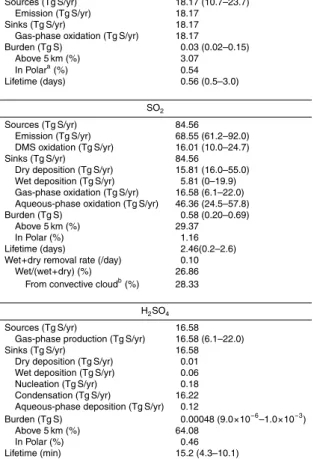
The simulated DMS burden is 0.03 Tg S with a lifetime of 0.56 day, which are at the low end of other model studies (DMS burden ranges from 0.02–0.15 Tg S, and lifetime ranges from 0.5–3.0 days) (Table 1, top). The smaller DMS burden in this study is

partly caused by high concentrations of NO₃ oxidant (not shown), especially at middle

to high latitudes during local summer, in this version of the model. About 3% of DMS

5

is located above 5 km, and 0.5% of DMS is located in the polar regions (south of 80◦S

and north of 80◦N, which comprises 1.5% of the earth’s surface area). The simulated

SO₂ burden is 0.58 Tg S with a lifetime of 2.5 days, which are at the high end of those

from other model studies (0.2–0.6 Tg S, and 0.6–2.6 days) (Table 1, middle). This is

consistent with the low dry deposition rate, which removes 15.8 Tg S yr−1 (compared

10

with 16.0–55.0 Tg S yr−1_{in other studies). Wet scavenging removes 5.8 Tg S yr}−1_{, 28%}

of which is from convective clouds. 29% of SO₂ is located above 5 km and 1.2% of

SO₂ is located in the polar regions. The simulated H₂SO₄ burden is 4.8×10−4Tg S

with a lifetime of 15.0 min, which are greater than other studies (Table 1, bottom). The

longer H₂SO₄ lifetime can be explained by a large amount of H₂SO₄ located above

15

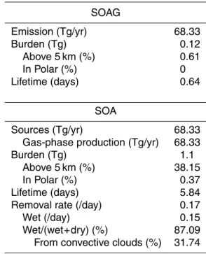
5 km (64%) where the condensation sink is low because of low preexisting aerosol surface area. The SOA gas burden is 0.12 Tg (Table 4). The only sink of SOA gas is

the condensation, which is 68.33 Tg yr−1_{. This gives a SOA gas lifetime of 0.64 days,}

although this value is somewhat misleading since the SOA gas and aerosol are in quasi-equilibrium (Liu et al., 2010).

20

The sulfate burden is 0.95 Tg S with a lifetime of 5.4 days, which is larger than the AeroCOM mean (0.66 Tg S and 4.12 days). The larger sulfate burden in MMF is caused

by a smaller wet removal rate coefficient (the inverse of the resident time) (0.16 day−1

vs. 0.22 day−1_{) (Table 2). The MMF model simulates a larger fraction of sulfate located}

above 5 km than that in AeroCOM (41% vs. 32%), with a much smaller fraction of

25

sulfate in the polar regions than that in AeroCOM (0.73% vs. 5.91%). The larger mass fraction above 5 km and smaller mass fraction in the polar regions are also true for

other aerosol species (see below). Difference in the partitioning of wet scavenging

(21)

GMDD

3, 1625–1695, 2010

M. Wang et al.

Title Page

Tables Figures

◭ ◮

Back Close

Full Screen / Esc

Discussion

P

a

per

|

Dis

cussion

P

a

per

|

Discussion

P

a

per

|

Discussio

n

P

a

per

|

MMF model and AeroCOM models may lead to these differences. Convective clouds

(i.e., convective updraft and downdraft, see Sect. 2.3.1) account for 29% of sulfate wet scavenging in the MMF model.

The global annual burden of black carbon (BC) is 0.12 Tg, which is only half of the AeroCOM mean (0.24 Tg) (Table 3, top). This is largely explained by a smaller BC

5

emission (7.5 Tg yr−1vs. 11.90 Tg yr−1), but also partly due to a somewhat shorter life-time (6.0 days vs. 7.1 days in AeroCOM). The shorter lifelife-time, compared to AeroCOM, is partially due to neglect of BC aging in the three-mode aerosol treatment. Convec-tive clouds account for about 32% of BC wet scavenging in the MMF model, which is slightly higher than that of sulfate aerosols and reflects the tropical biomass burning

10

sources of BC.

The primary organic carbon (POM) burden is 0.88 Tg, which is about half of the AeroCOM mean (1.7 Tg) (Table 3, bottom). This is mainly caused by a smaller POM

emission in the MMF model (48.5 Tg yr−1 _{vs. 96.6 Tg yr}−1 _{in AeroCOM). The POM}

lifetime is 6.7 days, similar to those in AeroCOM models. Convective clouds contribute

15

32% to POM wet scavenging. The simulated SOA burden is 1.1 Tg. Many of the AeroCOM models did not explicitly simulate SOA, but included some SOA sources in their POM emissions. Our 2.0 Tg burden for POM and SOA combined is fairly close to the AeroCOM mean POM burden. The SOA lifetime is 5.8 days (Table 4), which is

shorter than that of POM. This is caused by a large wet scavenging rate coe_fficient

20

of SOA, which can be explained by a larger hygroscopicity parameter of SOA (Liu et al., 2010) and by the fact that SOA is produced mainly in the low latitudes (with more precipitation) from the condensation of SOA (g) emitted near surface. The mass fraction of SOA located above 5 km is 38%, which is larger than that of POM (30%).

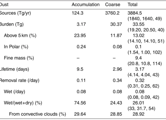
The simulated dust burden is 33.6 Tg, which is larger than the AeroCOM median

25

(20.50 Tg) (Table 5). This is mainly caused by the large dust emission in the MMF

model. The total dust emission is 3884 Tg yr−1 _{in CAM5, which almost doubles the}

median of the AeroCOM models (1840 Tg yr−1). The large dust emission in the MMF

(22)

GMDD

3, 1625–1695, 2010

M. Wang et al.

Title Page

Tables Figures

◭ ◮

Back Close

Full Screen / Esc

Discussion

P

a

per

|

Dis

cussion

P

a

per

|

Discussion

P

a

per

|

Discussio

n

P

a

per

|

dust emission parameterization as CAM5, without any tuning to the surface wind speed and soil moisture climatologies of the MMF model. The accumulation mode dust bur-den is 3.17 Tg and accounts for 9.4% of the total dust burbur-den, similar to the AeroCOM median (10.80%). The mass fraction of dust located above 5 km is 13%, which is sim-ilar to the AeroCOM median. Because of the larger particle size, the mass fraction of

5

dust above 5 km is less than that of sulfate, BC, and POM.

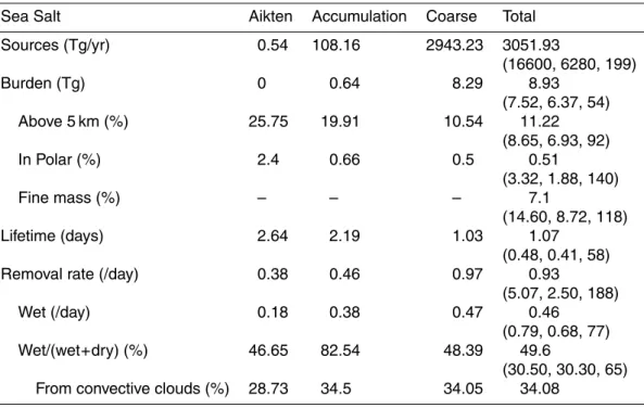
The simulated sea salt burden is 8.93 Tg, which is larger than the AeroCOM median (6.47 Tg) (Table 6). This is partly because sea salt in the MMF model has a longer lifetime (1.1 days) than that in the AeroCOM models (the median lifetime of 0.42 days). The fine mode sea salt mass fraction is 7.2%, which is similar to the median value

10

of the AeroCOM models (8.72%). Convective clouds account for 34% of sea salt wet scavenging, which is somewhat higher than that of the other aerosol species, and can be attributed to removal over tropical oceans.

3.2 Simulated global and vertical distributions of aerosols and gas species

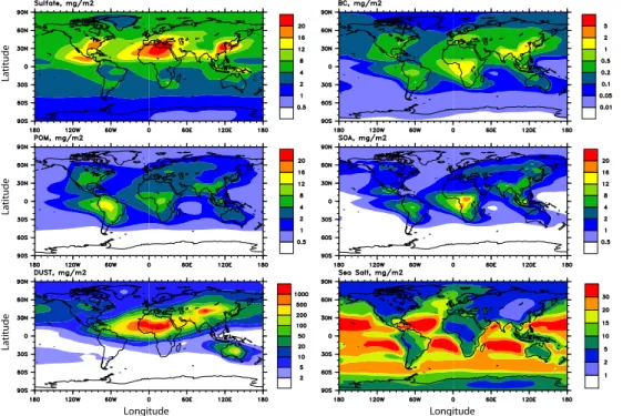
Figure 1 shows the vertically integrated annual mean column burdens for sulfate, BC,

15

POM, SOA, dust and sea salt. Sulfate burden is high over the strong source regions (e.g., East Asia, and the Eastern United States), and over the Northernmost Africa. The peak over the Northernmost Africa is caused by a combination of high oxidant concen-trations and reduced precipitation scavenging in that region. We noticed that a similar peak over the Northernmost Africa was also simulated in Mann et al. (2010). BC burden

20

is high over regions with strong fossil fuel emissions (East Asia and South Asia) and biomass burning emissions (Central Africa and South America). POM demonstrates a similar spatial pattern as BC, but the maximum POM burden is located over regions with strong biomass burning emissions, while the BC burden is slightly larger over regions with strong fossil fuel emissions than over regions with strong biomass

burn-25

(23)

GMDD

3, 1625–1695, 2010

M. Wang et al.

Title Page

Tables Figures

◭ ◮

Back Close

Full Screen / Esc

Discussion

P

a

per

|

Dis

cussion

P

a

per

|

Discussion

P

a

per

|

Discussio

n

P

a

per

|

dust source regions (40◦_–60◦_{N in the Western Pacific, and 10}◦_–30◦_{N in the Atlantic).}

Sea salt burden is high in the subtropics over both hemispheres, despite stronger sea salt emissions over the high latitudes. Less precipitation over the subtropics leads to the accumulation of sea salt. In the Southern Ocean, strong precipitation together with strong emissions leads to moderate sea salt burden.

5

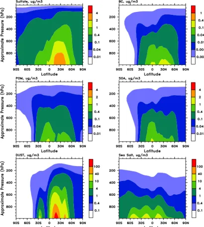
Figure 2 shows annual averaged zonal mean mass concentrations for sulfate, BC, POM, SOA, dust and sea salt. Sulfate zonal distribution demonstrates strong anthro-pogenic contributions in the NH and shows a strong zonal and vertical gradient. Sulfate

concentrations decreases by an order of magnitude from 30◦N to the poles. BC

con-centrations show two peaks, one located around 30◦_{N, due to fossil fuel emissions,}

10

and the other located in the tropics, due to biomass burning emissions. BC concen-trations are much lower in the Antarctic than in the Arctic region because of much less BC emissions in the SH middle and high latitudes. POM concentrations show two sim-ilar peaks as BC. Unlike BC, however, the peak in the tropics is stronger because the emission factor of POM from biomass burning is relatively higher than that from fossil

15

fuel. SOA concentrations have similar spatial distributions as POM. Dust concentra-tions show a stronger peak in the NH subtropics and a much weaker peak in the SH subtropics. The subtropic regions are located in the descending branch of Hadley cir-culation, where major deserts are located. Dust concentrations extend vertically into the upper troposphere. Simulated sea salt concentrations are stronger in the SH than

20

that in the NH, because of large open ocean areas in the SH. The peak located in 50◦S

is caused by strong surface wind speeds and large ocean areas over that region. Two

other peaks located over the subtropics are most likely caused by the less e_fficient wet

scavenging because of less precipitation over those regions.

Figure 3 shows annual mean aerosol number concentrations in the surface layer for

25

(24)

GMDD

3, 1625–1695, 2010

M. Wang et al.

Title Page

Tables Figures

◭ ◮

Back Close

Full Screen / Esc

Discussion

P

a

per

|

Dis

cussion

P

a

per

|

Discussion

P

a

per

|

Discussio

n

P

a

per

|

1000 cm−3_{. The accumulation mode aerosol number concentrations are also high in}

the polluted outflow regions over oceans (e.g., 40◦–60◦N over the East Pacific; tropical

Atlantic, and tropical East Pacific). The accumulation mode aerosol number

concen-trations can be as low as 40 cm−3 _{in remote areas. Aerosol number concentrations in}

the Aitken mode are high over land in the regions with strong sulfur emissions in the

5

transport and domestic sectors (e.g., the United States, Europe, and East Asia). This is not surprising since sulfur emissions in the transport and domestic sectors are the only sources of primary Aitken mode particles over land in the three-mode treatment. Aerosol number concentrations in the Aitken mode are lower over land in regions with strong biomass burning emissions. This is in part because all primary carbonaceous

10

aerosols are emitted into the accumulation mode in the three-mode treatment, and in part because high concentrations of accumulation mode particles slow down the generation of Aitken particles from nucleation. Over oceanic regions, aerosol number

concentrations in the Aitken mode are about 200–500 cm−3, which is in part from the

emission of Aitken mode sea salt particles and is in part from enhanced aerosol

nu-15

cleation due to low accumulation mode aerosol number concentrations. However, the Aitken mode number concentrations are lower over the oceanic regions with a large number of coarse mode particles (Fig. 4) (e.g., 0◦_–30◦_{N in the Atlantic, and 50}◦_–60◦_S

in the Southern Ocean), which is caused by the lower aerosol nucleation due to the

lower H₂SO₄ concentrations (not shown) from the condensation of H₂SO₄ onto the

20

coarse mode particles. The coarse mode number concentration is highest over the source regions of dust and sea salt particles and in the downwind of dust source

re-gions, and are generally lower than 10 cm−3.

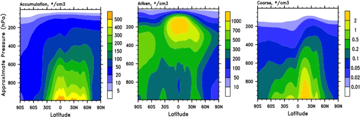
Figure 4 shows annual zonal mean aerosol number concentrations. Simulated ac-cumulation mode aerosol number concentrations show three peaks over the tropics,

25

30◦N, and 50◦N. The peak over the tropics results from biomass burning aerosols.

The peak at 30◦N is caused by pollution from South and East Asia, and the peak

around 50◦_{N is caused by pollution from Europe. The peak over tropics extends more}

(25)

GMDD

3, 1625–1695, 2010

M. Wang et al.

Title Page

Tables Figures

◭ ◮

Back Close

Full Screen / Esc

Discussion

P

a

per

|

Dis

cussion

P

a

per

|

Discussion

P

a

per

|

Discussio

n

P

a

per

|

burning emission which is injected at 0–6 km. The Aikten mode aerosol number con-centrations show a prominent peak in the tropical upper troposphere, where relative humidity is high and preexisting aerosol surface area is low, both of which favor the

binary homogeneous nucleation of H₂SO₄and H₂O. Another peak occurs in the

mid-dle troposphere over the SH high latitudes, which is associated with aerosol nucleation

5

in the austral summer (not shown). The spatial distribution of coarse mode aerosol number concentrations is similar to the spatial distributions of dust and sea salt mass concentrations (Fig. 2).

Figures 5 and 6 show the global distribution of CCN concentrations at 0.1% supersat-uration in the surface, and zonal mean CCN concentrations, respectively. The spatial

10

distribution of CCN concentrations is similar to that of the accumulation mode aerosol

number concentrations. One di_fference between the spatial distributions of CCN

con-centrations and the accumulation mode aerosol number concon-centrations is that CCN

concentrations peak in around 20◦–30◦N, but the accumulation mode number

concen-trations peak in the tropical regions. The peak in the tropical regions in the

accumula-15

tion mode number concentrations is caused by carbonaceous aerosol particles due to

biomass burning emission, but these carbonaceous aerosol particles are less efficient

to act as CCN than sulfate aerosol particles because carbonaceous aerosols are less hygroscopic.

4 Comparison with observations

20

4.1 Aerosol mass concentrations

Figures 7 and 8 compare modeled DMS and SO₂ vertical profiles with those from

three field experiments (PEM-Tropics A, September–October, 1996; PEM-Tropics B, March–April, 1999; TRACE-P, February–April, 2001). Vertical profile data are com-posites of observations binned into altitude ranges (Emmons et al., 2000). Model

25

(26)

GMDD

3, 1625–1695, 2010

M. Wang et al.

Title Page

Tables Figures

◭ ◮

Back Close

Full Screen / Esc

Discussion

P

a

per

|

Dis

cussion

P

a

per

|

Discussion

P

a

per

|

Discussio

n

P

a

per

|

observations show a strong gradient from the surface to the free troposphere. The model overestimates DMS concentrations in the boundary layer over the Japan coast and over Hawaii, and underestimates DMS concentrations in the free troposphere over

the China coast. Unlike DMS, observed SO₂ concentrations show a much weaker

gradient from the surface to the free troposphere. Over some locations, there are

5

even elevated SO₂layers in the middle and upper troposphere (e.g., Christmas-Island,

PEM-TROPICS A). Simulated SO₂ also demonstrates a much weaker gradient from

the surface to the free troposphere, and elevated SO₂layers are simulated over some

locations. In general, simulated SO₂concentrations are in reasonable agreement with

observations. However, the model overestimates SO₂concentrations over Christmas

10

Island and Guam, especially in the upper troposphere. The overestimation in the up-per troposphere is also evident in some other locations (e.g., Tahiti, PEM-TROPICS A). The overestimation in the middle and upper troposphere may indicate too strong verti-cal transport, and/or too weak in-cloud aqueous chemistry in the MMF model.

Figures 9 and 10 compare simulated annual mean surface SO₂and sulfate

concen-15

trations with observations from the United States Interagency Monitoring of Protected Visual Environment (IMPROVE) sites (http://vista.cira.colostate.edu/improve/), the Eu-ropean Monitoring and Evaluation Programme (EMEP) sites (http://www.emep.int), and the ocean network sites operated by the University of Miami (Arimoto et al., 1996;

Prospero et al., 1989; Savoie et al., 1989, 1993). Simulated SO₂ concentrations are

20

in reasonable agreement with observations at a large number of European sites, while

simulated SO₂concentrations are overestimated at the IMPROVE sites in the United

States. Sulfate concentrations are in reasonable agreement with observations. The agreement is particularly good in Europe (within a factor two) (Fig. 9). Over the United States, sulfate concentrations at most sites agree with observations within a factor of 2,

25