Comparison of different multi-objective calibration criteria of a conceptual rainfall-runoff model of flood events

(1)

HESSD

4, 1031–1067, 2007

Multi-objective calibration of a rainfall-runoffmodel

N. Chahinian and R. Moussa

Title Page

Abstract Introduction

Conclusions References

Tables Figures

◭ ◮

Back Close

Full Screen / Esc

Printer-friendly Version

Interactive Discussion

Hydrol. Earth Syst. Sci. Discuss., 4, 1031–1067, 2007 www.hydrol-earth-syst-sci-discuss.net/4/1031/2007/ © Author(s) 2007. This work is licensed

under a Creative Commons License.

Hydrology and Earth System Sciences Discussions

Papers published inHydrology and Earth System Sciences Discussionsare under open-access review for the journalHydrology and Earth System Sciences

Comparison of di

_ff

erent multi-objective

calibration criteria of a conceptual

rainfall-runo

_ff

model of flood events

N. Chahinian1,*and R. Moussa2

1

Agrocampus Rennes, Laboratoire Physique des Surfaces Naturelles et G ´enie Rural, 65 Rue de Saint Brieuc, 35042 Rennes, France

2

INRA, Laboratoire d’ étude des Interactions entre Sol – Agrosyst ème – Hydrosyst ème UMR LISAH AgroM-INRA- IRD, 2 Place Pierre Viala, 34060 Montpellier, France

*

now at: HydroSciences Montpellier, Universit ´e Montpellier 2, Case courrier MSE Place Eug `ene Bataillon, 34095 Montpellier Cedex 5, France

(2)

HESSD

4, 1031–1067, 2007

Title Page

Tables Figures

◭ ◮

Back Close

Full Screen / Esc

Abstract

A conceptual lumped rainfall-runoff_{flood event model was developed and applied on} the Gardon catchment located in southern France and various mono-objective and multi-objective functions were used for its calibration. The model was calibrated on 15 events and validated on 14 others. The results of both the calibration and validation

5

phases are compared on the basis of their performance with regards to six criteria, three global criteria and three relative criteria representing volume, peakflow, and the root mean square error. The first type of criteria gives more weight to strong events whereas the second considers all events to be of equal weight. The results show that the calibrated parameter values are dependent on the type of criteria used. Significant

10

trade-off_{s are observed between the di}ff_{erent objectives: no unique set of parameter} is able to satisfy all objectives simultaneously. Instead, the solution to the calibration problem is given by a set of Pareto optimal solutions. From this set of optimal solutions, a balanced aggregated objective function is proposed, as a compromise between up to three objective functions. The mono-objective and multi-objective calibration strategies

15

are compared both in terms of parameter variation bounds and simulation quality. The results of this study indicate that two well chosen and non-redundant objective func-tions are suffi_{cient to calibrate the model and that the use of three objective functions} does not necessarily yield diff_{erent results. The problems of non-uniqueness in model} calibration, and the choice of the adequate objective functions for flood event models,

20

emphasise the importance of the modeller’s intervention. The recent advances in au-tomatic optimisation techniques do not minimise the user’s responsibility, who has to chose multiple criteria based on the aims of the study, his appreciation on the errors induced by data and model structure and his knowledge of the catchment’s hydrology.

(3)

HESSD

4, 1031–1067, 2007

Title Page

Tables Figures

◭ ◮

Back Close

Full Screen / Esc

1 Introduction

It is common for hydrologists to model individual storm events at the catchment scale (e.g. Bates and Ganeshanandam 1990; Zarriello, 1998; Moussa et al., 2002; Jain and Indurthy, 2003), for flood forecasting, spillway design or flood protection schemes. The first important challenge that awaits the modeller in this task is to choose a

rainfall-5

runoff _{model, and to calibrate a set of parameters, that can accurately simulate a} number of flood events and related hydrographs shapes. Most of the models used currently for flood forecasting in France are lumped conceptual models (Garc¸on, 1996; Yang and Michel, 2000; Paquet, 2004) i.e. they have parameters which cannot, in gen-eral, be obtained directly from measurable catchment characteristics, and hence model

10

calibration is needed. Various calibration algorithms and procedures have been pre-sented in the literature extensively (Rosenbrock, 1960; Nelder and Mead 1965; Duan et al., 1992; Gan and Biftu, 1996; Yapo et al., 1998; Vrugt et al. 2003a and 2003b; see a review in Gupta et al., 2003). Although they diff_{er in the ways they seek the optimal} value, they all aim at minimising or maximising an objective function. It is important to

15

note that, in general, trade-off_{s exist between the di}ff_{erent objective functions. For} in-stance, when using the bias as an objective function, one may find a set of parameters that provides a very good simulation of volume, but a poor simulation of the hydrograph shape or peak flow, and vice versa. Conventional objective functions such as the root mean square error, the Nash and Sutcliff_{e (1970) e}ffi_{ciency coe}ffi_{cient, or the index}

20

of agreement (Willmott, 1981) tend to emphasize the high flows, and consequently, are oversensitive to extreme values and outliers (Legates and McCabe, 1999). On the opposite, the mean absolute percent error tends to emphasize the low flows (Yu and Yang, 2000).

However, in most real world applications, models are used to reproduce the entire

25

(4)

HESSD

4, 1031–1067, 2007

Title Page

Tables Figures

◭ ◮

Back Close

Full Screen / Esc

would be advisable to take into account various objective functions by considering the calibration problem in a multi-objective framework (Yapo et al., 1998; Madsen, 2000). Most of the studies related to multi-objective calibration have investigated the use of two objective functions and few ones have looked into the use of three or more func-tions (Schoops et al., 2005, Parajka et al., 2007). In this study we will extend the use of

5

the balanced aggregative function suggested by Madsen (2000) to three objective func-tions. In addition, while most of these studies have dealt with continuous simulations, we will investigate multi-objective calibration issues related to event based modelling.

Hence, the objective of this paper is to develop an event based lumped conceptual rainfall-runoff _{model and then to compare mono-objective and multi-objective}

calibra-10

tion approaches. The emphasis is put on the impact of the selected objective functions on the actual hydrograph shapes and simulation errors rather than on the calibration algorithm as several studies have already investigated this issue (Yu and Yang, 2000; Johnsen et al., 2005; Tang et al., 2006). The Gardon catchment located in southern France is used in the applications because of the recurrent flooding problems its

in-15

habitants encounter yearly. The objective functions used in this study can be divided in two broad categories: global and relative. Given the diversity of the flood events to be modelled such an approach was deemed necessary as the first type of criteria gives more weight to strong events whereas the second considers all events to be of equal weight. For each category, three diff_{erent objective functions are considered:}

20

volume conservation which is important for gauging problems, peakflow reproduction which is essential for flood applications and the root mean square error as a measure of the global agreement between the simulated and observed curves. The paper is organised in four sections: i) model presentation; ii) formulation of the calibration cri-teria; iii) presentation of the study zone, and iv) model performance analysis based on

25

mono-objective and multi-objective calibration.

(5)

HESSD

4, 1031–1067, 2007

Title Page

Tables Figures

◭ ◮

Back Close

Full Screen / Esc

2 The lumped conceptual rainfall-runoffmodel

Since the 1960s, lumped, conceptual rainfall-runoff_{models have been used in} hydrol-ogy (e.g. Crawford and Linsley, 1966; Cormary and Guilbot, 1969; Duan et al., 1992; Bergstr ¨om, 1995; Donigan et al., 1995; Havnø et al., 1995). These models consider the catchment as an undivided entity, and use lumped values of input variables and

pa-5

rameters. For the most part (for a review, see Fleming, 1975; Singh, 1995), they have a conceptual structure based on the interaction between storage elements representing the diff_{erent processes with mathematical functions to describe the fluxes between the} stores.

The modelling approach followed herein will be lumped and the catchment will be

10

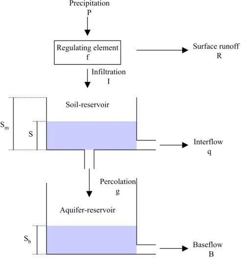
considered as a single entity. A two-reservoir-layer model has been developed to rep-resent the catchment on the basis of the CREC model (Cormary and Guilbot, 1969) and the Diskin and Nazimov (1995) production function (Fig. 1). Evaporation is not rep-resented since the purpose of the model is to simulate individual flood events during which evapotranspiration is negligible. The first layer, noted “soil-reservoir”, represents

15

the upper soil layer and controls surface runoff_{, infiltration, interflow and percolation.} The second layer, noted “aquifer-reservoir”, represents the aquifer where mainly base flow occurs. A unit hydrograph transfer function is used to route flows to the outlet. The output of the model will be a simulated hydrograph which will be compared to the original measured hydrograph to assess model performance. A general description of

20

each procedure is given below.

2.1 The production function

A regulating elementf separates the precipitationP into surface runoff_R_{, and} infiltra-tionI. The soil-reservoir element has one input, the infiltrationI, and two outputs, the lateral interflow q, and the vertical flow g which represents the percolation from the

25

upper soil layer to deeper layers. The state variable of the regulating element, denoted

(6)

HESSD

4, 1031–1067, 2007

Title Page

Tables Figures

◭ ◮

Back Close

Full Screen / Esc

Diskin and Nazimov (1995) relationship

f =_f

0−(f0−fc)

S

S_m (1)

wheref0 [LT− 1

] is the maximum infiltration capacity, f_c [LT−1] the minimum infiltration capacity, andSm [L] the maximum storage in the soil-reservoir layer. The value of fc characterises the soil’s infiltration capacity at saturation, and the term (S/Sm)

charac-5

terises the soil moisture. The two outputsIandRof the regulating element depend on the value of the state variablef and on the value of the input P, at the same instant according to the following equations

IfP < f thenI=_P _and_R =₀ ₍₂₎ IfP > f thenI=_f _and_R=_P ₋_f ₍₃₎

10

The two outputs of the soil-reservoir,qandg, are calculated function of a parameterb

(with 0≤b≤1) and the term (S/Sm)

q=_f

cb

S

S_m andg=fc(1−b) S

S_m (4)

It should be noted that the sumq+_g=_f

cSSm is independent of the parameter b and

ver-ifies the soil-reservoir output of the Diskin and Nazimov (1995) model. As the storage

15

S approaches the threshold value S_m, both the infiltration capacity f and the sum q+_g tend to the same value f_c.

The aquifer-reservoir has one input, the percolation g, and one output, the base flow B [LT−1], which is calculated function of the aquifer-reservoir level S_b using a linear relation

20

B=_kS

b (5)

where k[T−1] is a constant characterizing the recession curve of the aquifer. In order to reduce the number of parameters, the aquifer-reservoir hasn’t a maximum storage

(7)

HESSD

4, 1031–1067, 2007

Title Page

Tables Figures

◭ ◮

Back Close

Full Screen / Esc

depth. The value of the state variable S_bof the aquifer-reservoir is obtained using the continuity equation

d S_b

d t =g(t)−B(t) (6)

2.2 The transfer function

A transfer function is used to route the rainfall excess to the catchment outlet. A unit

5

hydrograph linear model, based on a Hayami (1951) kernel function, which is a reso-lution of the diff_{usive wave equation, was used to simulate the transfer of the sum of} (R +_q+_B_{) to the outlet (Moussa and Bocquillon, 1996). Let}_I₍_t_{) [}_L3_T−1_{] be the input} hydrograph

I(t)=₍_R+_q+_B₎_.A ₍₇₎

10

whereA[L2] is the catchment area. LetO(t) be the routed hydrograph at the outlet

O(t)= t

Z

0

I(τ).H(t−τ).d τ (8)

withH(t) the Hayami kernel function defined as

H(t)=w.z

π

1/2

· exp

z₍2−_wt−w_t)

(t)3/2 with

Z∞

0

H(t).d t=₁ ₍₉₎

where w[T] is a time parameter that represents the centre of gravity of the unit

hy-15

drograph, z [dimensionless] a form parameter, π=_{3.1416 and} _t _{the time [T]. For low} values ofz (i.e.z=_{1, 2 or 5), the unit hydrograph represents both translation and di}ff u-sivity (resolution of the diff_{usive wave equation), while for high values of}_z_(i.e._z=_{20, 50} or 100), the unit hydrograph tends to represent only a translation equal tow(resolution of the kinematic wave equation).

(8)

HESSD

4, 1031–1067, 2007

Title Page

Tables Figures

◭ ◮

Back Close

Full Screen / Esc

2.3 Model properties and parameters

The input rainfallP is usually given as a function of time in the form of a histogram using a fixed time interval. Consequently, the other variables are also presented as functions of time, and the computations are carried out for the same fixed time inter-val. The regulating element f and the soil-reservoir element are linked by a feedback

5

path transmitting information about the state of the storage element to the regulating element. The regulating element is related to the soil-reservoir element by the fact that one of its outputs is the input of the soil-reservoir element. It is also related to the transfer function by the fact that its outputR is one input of the transfer function.

Computations start at an instant adopted as zero time t=_{0, with a known, or an}

10

assumed, initial value of the soil-reservoirS0and the aquifer-reservoir Sb0 at the start of that time interval. For each flood event, the value ofS0is defined according to the 5-day antecedent rainfallR5d corresponding to three classes (Soil Conservation Service, 1972)

IfR5d <10 mm thenS0=0.25Sm (10)

15

If 10< R5d <30 mm thenS0=0.50Sm (11)

IfR5d >30 mm thenS0=0.75Sm (12)

At the beginning of the rainfall event, the measured discharge Qo(0) att=_{0 is the sum} of the lateral interflowq and the base flow B. Using Eqs. (4) and (5), and substituting S by S₀, the initial value of the aquifer-reservoirSb0is calculated as

20

Sb0= 1

k

_Qo

(0)

A −fcb S0

Sm

(13)

For each time interval, the three state variablesf(t) which separates rainfall into surface runoff_{and infiltration, the level}_S₍_t_{) in the soil-reservoir and the level}_S

b(t) in the aquifer-reservoir are calculated from the known values of the variables at the beginning of the

(9)

HESSD

4, 1031–1067, 2007

Title Page

Tables Figures

◭ ◮

Back Close

Full Screen / Esc

time interval and the rainfall input to the model during the interval. The values of the other variables at the end of the computation time interval are derived from the value of the three state variables by using the equations above.

The model needs : i) five parameters for the production function, the minimum value of the infiltration capacityfc, a coefficient “a” such as maximum value of the infiltration

5

capacityf0=afc(witha>1), the maximum level of the soil-reservoir Sm, the parameter

bof the lateral interflow, and the parameterkof the aquifer-reservoir’s recession curve, ii) two parameters for the transfer function, the lag time w and the shape parameterz

and iii) two initial conditions S0 and Sb0 calculated function of the 5-day antecedent rainfallR5d and the measured dischargeQo(0) att=0.

10

3 Formulation of calibration criteria

The objective of model calibration is to select parameter values so that the model sim-ulates the measured hydrograph as closely as possible. Our aim is to consider multiple objectives that measure diff_{erent aspects of the hydrological response (Madsen, 2000):} i) a good agreement between the average simulated and observed runoff_{volume (i.e. a}

15

good water balance); ii) a good agreement of the peak flows; iii) a good overall agree-ment of the hydrograph shape.

When a calibration procedure is used, the quality of the final model parameters will depend on the structure of the model, the power of the optimisation algorithm, the quality of the input data, and the estimation criteria or objective functions used in the

20

(10)

HESSD

4, 1031–1067, 2007

N. Chahinian and R. Moussa Title Page Abstract Introduction Conclusions References Tables Figures ◭ ◮ ◭ ◮ Back Close

Full Screen / Esc

3.1 The objective functions

The objective functions used in this study include both relative and absolute error mea-sures as suggested by Legates and McCabe (1999). The selected criteria can be di-vided in two broad categories: “global” which gives more weight to strong flood events and “relative” which considers all events to be of equal weight. For each category, three

5

diff_{erent objective functions were considered: volume conservation, peakflow} predic-tion, and the root mean square error (RMSE) which to a certain extent is comparable to the widely used Nash and Sutcliff_{e (1970) e}ffi_{ciency measure:}

1.The global volume errorV_g and the relative volume errorV_r

V_g=

N P

i=1

(Ls_i−Lo_i)

N

P

i=1

n_i

andV_r=1

N

X

i=1

Lsi−Loi

Lo_i (14) 10

whereNis the total number of flood events used for calibration,i an index representing a flood event (1≤i≤N), and for each flood event i : n_i the number of time steps, Lo_i the observed runoff_{depth and Ls}

ithe simulated runoffdepth.

2. The global root mean square error RMSEg and the relative root mean square error RMSE_r

15

RMSE_g =

      N P

i=1 ni P

j=1

Qoi j−Qsi j

2

N

P

i=1

ni       1 2

and RMSE_r = 1

N

X

i=1

  1 ni ni X

j=1

Qo_{i j}−Qs_{i j}2 

 1 2

(15)

wheren_i is the number of time steps in the flood event i, j is an index representing the time step in a flood eventi (1≤j≤n_i), Qo_{i j} the observed discharge at timej in the flood eventi and Qs_{i j} the simulated discharge at timejon the flood eventi.

(11)

HESSD

4, 1031–1067, 2007

Title Page

Tables Figures

◭ ◮

Back Close

Full Screen / Esc

3. The global peakflow P_g and the relative peakflowP_r

P_g = 1

N

X

i=1

|(Qxs_i −Qxo_i)|andP_r = 1

N

X

i=1

Qxsi−Qxoi

Qxo_i

(16)

whereQxoi is the observed peak flow of discharge in the flood eventi andQxsi is the simulated peak flow of discharge in the flood eventi.

The six objective functions, Vg, Vr, RMSEg, RMSEr, Pg and Pr, are positive

func-5

tions, and the optimum value of the parameters corresponds to the minimum value of each “0”. A mono-objective calibration procedure was undertaken separately with each of the six criteria. Most model calibration procedures suff_{er from the same problems,} namely the existence of multiple optima and the presence of high interaction or correla-tion between subsets of fitted model parameters. In order to avoid these, no automatic

10

calibration procedure was undertaken, instead a grid-based calibration procedure was carried out to locate the optimum, and over 50000 simulations were run to calibrate the model using a progressively finer grid.

3.2 Multi-objective calibration procedures

When using multiple objectives, the calibration problem can be stated as follows

(Mad-15

sen, 2000)

min{F1(θ), F2(θ), . . ., Fm(θ)] withθ∈Θ (17) where F_i(θ) (i = _{1, 2 . . . , m) are the di}ff_{erent objective functions. The optimisation} problem is constrained becauseθis restricted to the feasible parameter spaceΘ_{. The} parameter space is usually defined as a hypercube by specifying lower and upper limits

20

(12)

HESSD

4, 1031–1067, 2007

Title Page

Tables Figures

◭ ◮

Back Close

Full Screen / Esc

The solution of Eq. (17) will not, in general, be a single unique set of parameters but will consist of the so-called Pareto set of solutions according to diff_erent trade-off_{s between the di}ff_{erent objectives (Gupta et al., 2003). The parameter space can} be divided into “good” (Pareto optimal) and “bad” solutions, and none of the “good” solutions can be said to be “better” than any of the other “good” solutions (Madsen,

5

2000). A member of the Pareto set will be better than any other member with respect to some of the objectives, but because of the trade-off_{between the di}ff_{erent objectives} it will not be better with respect to other objectives. In practical applications, the entire Pareto set may be too expensive to calculate, and one is only interested in part of the Pareto optimal solutions.

10

When dealing with the multi-objective calibration, the problem is usually transformed into a single-objective optimisation problem by defining a scalar that aggregates the various objective functions (Madsen, 2000; Parakja et al., 2007) such as the Euclidean distance

F_agg(θ)=h₍_F₁₍_θ₎+_A₁₎2+₍_F₂₍_θ₎+_A₂₎2+_...+₍_F

p(θ)+Ap)2

i1/2

(18)

15

whereAi are transformation constants, reflecting the priorities assigned to the different objective functions. Herein, the balanced aggregated objective function suggested by Madsen (2000) was applied. In this case, the transformation constants in Eq. (18) are automatically calculated so that all (Fi(θ) +Ai) have about the same distance to the origin near the optimum.

20

The multi-objective calibration procedure was first undertaken for each of the couples within the same function type i.e. (Vg and Vr), (RMSEg and RMSEr) and (Pg and Pr). Then, we crossed two “global” criteria i.e. (V_g and RMSE_g,), (V_g andP_g), (RMSE_g and

P_g), and two “relative” criteria (V_r and RMSE_r), (V_rand P_r) and (V_rand RMSE_r), In the last step, the calibration was carried out function of the triples (Vg, RMSEg and Pg) and

25

(V_r, RMSE_r andP_r).

(13)

HESSD

4, 1031–1067, 2007

Title Page

Tables Figures

◭ ◮

Back Close

Full Screen / Esc

4 The study site

4.1 Catchment description

The Gardon d’Anduze is a 543 km2 Mediterranean catchment located in Southern France. It has a highly marked topography consisting of high mountain peaks, nar-row valleys, steep hillslopes and a herring-bone shaped channel network. The

high-5

est point is the Mont Aigoual at 1567 m a.s.l. and the outlet is located at Anduze at 123 m a.s.l. The catchment’s soils developed essentially on metamorphic (64% of the catchment area) and granitic terrains. The substrate is made of shale and crystalline rocks overlain by silty clay loams (83% of the catchment area) and sandy loam top soil. The vegetation is dense and composed mainly of beech and chestnut trees, holm oaks

10

and garrigue, conifers, moor, pasture and cultivated lands. These vegetation classes are typical of Mediterranean forests.

Rainfall data for the 1977–1984 period were obtained on paper medium from the “Direction D ´epartementale de l’Equipement du Gard” of the French Ministry of Equip-ment on seven rain gauge stations. The “Direction D ´eparteEquip-mentale de l’EquipeEquip-ment

15

du Gard” provided also analogue streamflow hydrographs at the outlet at Anduze (Moussa, 1991). Mean rainfall was calculated as the arithmetic mean of the seven rain gauges. The Gardon region is characterized by the highest rainfall intensities recorded in France e.g. a maximum daily rainfall of 608 mm was recorded on the Mont Aigoual during 24 h on 30–31 October 1963. The analysis of long rainfall time series shows

20

that a daily rainfall of 70 mm has a return period of 1 year and daily rainfall of 170 mm has a return period of 100 years. The conjunction of high intensity rainfall, shallow soils and steep slopes produce very devastating floods in autumn.

4.2 Characteristics of the studied flood events

Flood events from the 1977–1984 period were selected based on a continuous rainfall

25

(14)

HESSD

4, 1031–1067, 2007

Title Page

Tables Figures

◭ ◮

Back Close

Full Screen / Esc

at an hourly time step (Moussa, 1991). In total, 29 events were retained: the event durations range between 24 h and 108 h, the total rainfall between 50 mm and 300 mm, the total runoff_{between 9 and 166 mm, the runo}ff_coeffi_{cients between 15% and 67%,} and the initial discharge between 3 and 92 m3s−1. Figure 2 shows the relations be-tween the total rainfall, the total runoff_{depth, runo}ff_coeffi_{cient, peakflow, and the initial}

5

discharge. No clear correlation can be seen between them i.e. the most important rainfall events in terms of precipitation volume aren’t necessarily those that have the highest runoff_coeffi_{cients or peakflow. The initial discharge value which represents the} catchment’s moisture condition doesn’t seem to yield linear trends either. This finding is typical of Mediterranean climatic conditions where short duration and high intensity

10

rainfall events are often the cause of the most important runoff_{events in terms of both} runoff_{depth and peakflow.}

Fifteen events, corresponding to the 1977–1979 period, were chosen for calibration and the remaining fourteen, corresponding to the 1980–1984 period, were used for validation (Fig. 2). Both data sets are representative of the various hydrological

be-15

haviours observed on the catchment. They cover all climatic seasons and display a large spectrum of rainfall intensity, peakflow and runoff_coeffi_{cient values.}

5 Mono- and mutli-objective calibration and validation results

For the fifteen events of the calibration period, a number of tests were carried out in order to optimise the parameters first using mono-objective functions, and then to

20

estimate the Pareto front and analyse the trade-off_{s between the di}ff_{erent objectives} when using two- or three-objective approaches. We defined a lower and an upper variation bound for each parameter. For all numerical tests, the hypercube search space shown in Table 1a was used.

(15)

HESSD

4, 1031–1067, 2007

Title Page

Tables Figures

◭ ◮

Back Close

Full Screen / Esc

5.1 Results of the mono-objective calibration procedure

The calibrated parameter values for each of the six objective functionsV_g,V_r, RMSE_g, RMSE_r,P_g andP_r, are presented in Table 1b. Results show that the parameters vary considerably depending on the objective function used.

For the production function, the soil-reservoir maximum capacityS_mranges between

5

9 and 71 mm; this appears to be a small value if it is supposed to represent the storage in the root zone. The parameterfc, which represents the soil’s infiltration capacity at natural saturation, varies between 0.29×10−5 and 2.6×10−5ms−1 and compares well with the values estimated when using Rawls and Brakenseik’s (1989) pedotransfer function. It is interesting to note that the two empirical parametersa and b have the

10

widest span, probably because these parameters are used to compensate for the er-rors made on the remaining parameters of the production function. Indeed, even when using conceptual models, modellers tend to be less permissive with parameters that can evoke physical characteristics or be assimilated to such. As a direct consequence, such parameters, even in an un-constrained calibration procedure, will be allowed to

15

vary in a tighter interval.

The transfer function has two parameters w and z. The travel time values of w obtained through the use of V_g and V_r (w=_{21–23 h) are clearly overestimated both} in comparison with the observation data (the basin response time ranges between 3 and 9 h) and the values obtained through RMSEg, RMSEr,Pg andPr (w=3–4 h). This

20

is because the two volume criteria V_g and V_r are less sensitive to the hydrograph’s global shape and consequently to the parameters of the transfer function. The second parameter of the transfer functionz ranges between 3 and 17. These values highlight the importance of the diff_{usive factor.}

For most parameters the use of RMSE_g or RMSE_r yields close results. However,

25

when using Pg or Pr, the calibrated parameters differ from those obtained with Vg,

(16)

HESSD

4, 1031–1067, 2007

Title Page

Tables Figures

◭ ◮

Back Close

Full Screen / Esc

the whole shape of the hydrograph, whileP_g andP_r refer to a single point representing peakflow.

No unique solution to the mono-objective problem is found and an “equifinality” of parameter sets can be seen as stated by Beven and Binely (1992) and Beven (1992 and 1993) i.e. many diff_{erent parameter combinations give acceptable solutions.}

5

5.2 Results of the multi-objective calibration procedure when crossing two objective functions

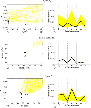
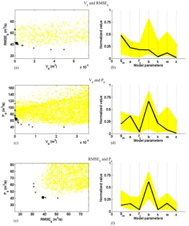
The results of the multi-objective calibration obtained when crossing two objective func-tions are shown in Figs. 3, 4 and 5. In Fig. 3, the calibration is based on two objective functions, the global volume error V_g and the relative volume error V_r (Fig. 3a), the

10

global RMSE_g and the relative RMSE_r (Fig. 3c) and the global peakflow P_g and the relative peakflowPr (Fig. 3e). Figures 3a, c and e show the objective function values corresponding to the evaluated parameter sets for two diff_{erent objective functions. The} Pareto optimal front (indicated by a star “*” on Figs. 3a, c and e) is identified, and finally the balanced aggregated objective function (indicated by an arrow on Figs. 3a, c and

15

e) is calculated. The mono-objective optimisation provides the tails of the Pareto front, and the optimisation based on the balanced aggregated measure approximates the balanced central part of the Pareto front.

The estimated Pareto front for the calibration ofV_g andV_r (Fig. 3a) presents a trade-off_{. A very good calibration of}_V

g (corresponding toVg=0) provides a bad calibration of

20

V_r (V_r=_{16.7%), and vice-versa (}_V

g=0.166×10− 4

m3forV_r=_{8.7%). The same comment} can be made about P_g and P_r: P_g=_{40.3 m}3_s−1_when _P

r=18.3% andPg=58.0 m 3

s−1 when P_r=_{13.3 %. This result is not surprising as peakflow refers to instantaneous} values that are both diffi_{cult to determine and simulate. The Pareto front of RMSE}

gand

RMSE_r shows a high correlation. This can be explained by the fact that the majority

25

of flood events have similar duration (48 to 96 h) and consequently the two objective functions presented in Eq. (15) tend to be similar.

(17)

HESSD

4, 1031–1067, 2007

Title Page

Tables Figures

◭ ◮

Back Close

Full Screen / Esc

The variation of the optimum model parameter sets along the Pareto front is shown in grey in Figs. 3b, d and e for the multi-objective calibration of (Vg and Vr), (RMSEg and RMSE_r) and (P_g andP_r) respectively. The parameter values are normalised with respect to the upper and lower limits given in Table 1a so that the range of all nor-malised parameters is between 0 and 1. For the calibration ofVg and Vr (Fig. 3b), a

5

remarkably large span is observed in the parameter values when moving along the Pareto front. The range is larger than 50% for the main parametersS_m,a,b,w andz. The compromised solution using the balanced aggregated function (Eq. 18) is shown in bold on Figs. 3b, d and e, and the corresponding values of the calibrated parameters are given in Table 1c1. The calibrated parameters of the compromised solution of (V_g

10

andVr) in Table 1c1 range within the interval delimited by the calibrated parameters of

V_g and V_rseparately (Table 1b). Similar results are observed for (RMSE_g and RMSE_r) and for (P_g andP_r).

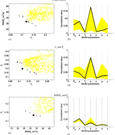
Figure 4 shows results when crossing two “global” criteria (Vg and RMSEg; Figs. 4a, b), (V_g andP_g; Figs. 4c, d) and (RMSE_g andP_g ; Figs. 4e, f) and Fig. 5 shows results

15

when crossing two “relative” criteria (V_r and RMSE_r; Figs. 5a, b), (V_r andP_r; Figs. 5c, d) and (RMSE_r and P_r; Figs. 5e, f). Again, we observe significant trade-off_{s for the} three cases of Fig. 4 :

– V_g=_{0 when RMSE}

g=65.5 m 3

s−1andV_g=_5.0×10−5_m3_{when RMSE}

g=31.0 m 3

s−1 (Fig. 4a);

20

– Vg=0 whenPg=92.4 m3s−1andVg=23.8×10−5m3whenPg=40.3 m3s−1(Fig. 4c);

– RMSE_g=_{31.0 m}3_s−1 _when _P

g=61.6 m 3

s−1 and RMSE_g=_{50.9 m}3_s−1 _when

P_g=_{40.3 m}3_s−1_{(Fig. 4e).}

Comparable results are obtained with the relative criteria in Figs. 5a, c and e. The variation of the optimum model parameter sets along the Pareto front for the

multi-25

(18)

HESSD

4, 1031–1067, 2007

Title Page

Tables Figures

◭ ◮

Back Close

Full Screen / Esc

(RMSE_g andPg; Fig. 4f) and (RMSEr and Pr; Fig. 5f). Figures 3 to 5 indicate that the global volume criteria (Vg) is the most insensitive i.e. volume conservation can be easily respected with a number of septuplet combinations. This translates into a somehow flat Pareto front (Figs. 3a, 4a, b). In comparison RMSE and peakflow produce sharper fronts; RMSE seems to be the most restrictive of the tested criteria. The relative criteria

5

seem to yield sharper fronts than the global criteria which seem to be controlled by the extreme events.

In comparison with the mono-objective calibration, the use of a multi-objective cali-bration technique seems to yield tighter variation intervals. These findings are in ac-cordance with those of Engeland et al. (2006). The variation ranges we obtained for

10

the multi-objective calibration are smaller than those reported in Schoops et al. (2005) and Madsen (2000) who had respectively 3 and 2 additional parameters to calibrate. However, the number of free parameters cannot be the only explanation behind the wider variation spans as Gupta et al. (2003) obtained tighter intervals when calibrating the 13 parameters of the SAC-SAM model.

15

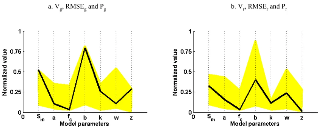
5.3 Results of the multi-objective calibration procedure when crossing three objective functions

The same methodology was extended in order to combine three objective functions. Figure 6 shows the results obtained when crossing the three global objective functions (V_g, RMSE_g andP_g; Fig. 6a), and the three relative objective functions (V_r, RMSE_r and

20

Pr; Fig. 6b). Results show comparable parameter variation ranges for both (Vg, RMSEg andP_g) and (V_r, RMSE_r andP_r).

For the optimal solution (Table 1d), the soil-reservoir maximum capacityS_m is equal to 172 mm when crossing (Vg, RMSEg andPg) and 225 mm when crossing (Vr, RMSEr and P_r). This value is more representative of the storage in the root zone. For both

25

combinations (V_g, RMSE_g and P_g) and (V_r, RMSE_r and P_r), the optimal parameterf_c

ranges between 5.5×10−5 and 7.4×10−5ms−1, and compares well with pedotransfer

(19)

HESSD

4, 1031–1067, 2007

Title Page

Tables Figures

◭ ◮

Back Close

Full Screen / Esc

functions. It is interesting to note that the two empirical parameters a and b still have the widest span. The travel time values of w obtained range between 3 and 4 h and correspond to the approximate lag time of the basin during intense flood events, while the dimensionless shape parameterz, ranges between 14 and 28.

The parameter variation ranges are comparable to those obtained when using only

5

two functions. The parameters that vary mostly between the two combinations areb,k

andz. The parametersbandk are clearly linked to each other as they both control the “outward” fluxes and can be used to correct possible flow over-estimation by increasing percolation and interflow. Data on water levels both in the unsaturated and saturated zones could have been useful in constraining these parameters further. Unfortunately

10

such data were unavailable for the studied period.

5.4 Validation and uncertainty analysis

As the “relative” and “global” criteria gave comparable results and interpretation, we choose to validate the results of the “relative” criteria (V_r, RMSE_r and P_r) which are less sensitive to extreme events.

15

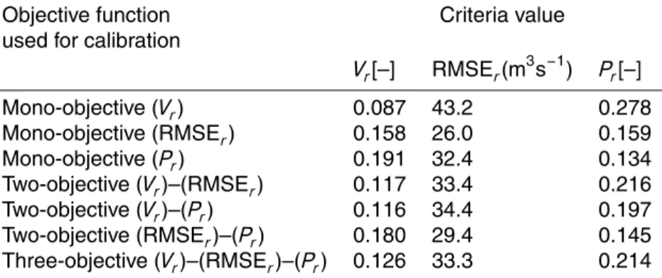
To compare the calibration procedures, we computed the value of each objective function (Table 2). It is not surprising that the values of V_r, RMSE_r and P_r are mini-mal when mono-objective calibration are conducted function of each of these criteria:

V_r=_{8.7%, RMSE}

r=26.0 m 3

s−1andP_r=_{13.4%. The maximal value of}_V

r=19.1% is ob-tained when using a mono-objective calibration minimising P_r; the maximal value of

20

RMSE_r=_{43.2 m}3_s−1 _{is obtained when using a mono-objective calibration minimising} Vr; and the maximal value ofPr=27.8% is also obtained when using a mono-objective calibration minimisingV_r. Once again the use of a volume based criterion is restrictive while the use of RMSE can yield relatively acceptable results for peakflow and vice versa. The sensitivity of the RMSE criterion to peakflow has already been reported by

25

many authors (Parada et al., 2003; Yapo et al., 1998) and our findings are similar to theirs.

(20)

HESSD

4, 1031–1067, 2007

Title Page

Tables Figures

◭ ◮

Back Close

Full Screen / Esc

indicated above. However, it is interesting to note that for all three criteria, the maximal errors values obtained with the multi-objective methods are always lower than those obtained when using a mono-objective calibration in which the given criterion is not considered. Finally the combination of (V_r, RMSE_randP_r) gives a reasonable compro-mise between the three criteria with Vr=12.6%, RMSEr=33.3 m

3

s−1 and Pr=21.4%.

5

These values are quite comparable to those obtained when using just two objective functions i.e.V_r, RMSE_r.

To further compare the performance of the calibration procedures, we computed the relative error on both runoff_{depth and peakflow: for a given event i, the error on runo}ff depth and peakflow are defined respectively by ε_vi=₍_Ls

i-Loi) / Loi and εQi=(Qxsi

-10

Qxoi)/Qxoi. Let εV and εQ be the mean of εvi and εQi respectively. The quantities

εV and εQ represent the bias of runoff depth and peakflow predictions. Table 3 il-lustrates the findings when using either mono and multi-objective method (i.e. two or three objective functions) and shows that εV and εQfall within similar ranges for two-or three-objective functions. It is wtwo-orthy to note that the greatest errtwo-ors on runoff_depth

15

are obtained through the use of a peakflow criterion while the greatest errors on peak-flow are caused by the use of a volume criterion. Apart from two cases, the error on runoff_{depth is acceptable (}_<_{5%) while, not surprisingly, the error on peakflow is far} higher (>10%) but less than 27%. In addition, the model seems to have a tendency to overestimate runoff_{depth and to underestimate peaflow.}

20

The best compromise between both errors is reached by using the parameters ob-tained through the multi-objective calibration with three functions (V_r-RMSE_r-P_r) but the combination ofV_r and RMSE_r gives once again comparably good results. In this instance the use of two “well” chosen and complementary objective functions seems to be suffi_{cient for runo}ff_{simulation. However, the lack of soil-moisture and groundwater}

25

data prevents us from extending our results to the other vertical components of the model.

Figure 7 compares the measured and simulated runoff _{depths (Fig. 7a) and the} measured and simulated peakflows (Fig. 7b) obtained when using the parameters of

(21)

HESSD

4, 1031–1067, 2007

Title Page

Tables Figures

◭ ◮

Back Close

Full Screen / Esc

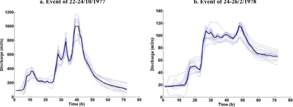
the balanced aggregated objective function (Vr, RMSEr and Pr) given in Table 1d. It can be seen that the model gives similar results both for the calibration and validation periods. An illustration of the equifinality problem is shown in Fig. 8 where simulated hydrographs are obtained using the parameters corresponding to the entire Pareto front of (Vr, RMSEr and Pr). The results indicate that the hydrographs are also well

5

simulated for high (Fig. 8a) and low intensity events (Fig. 8b). The figure shows clearly that many diff_{erent parameter sets, may produce equally good simulations according} to the three objective functions.

6 Discussion and conclusion

A conceptual lumped event based rainfall-runoff _{model, coupling a production and a}

10

transfer function, was developed and applied on the Gardon catchment in southern France. The model has seven free parameters which need to be calibrated. The model was calibrated on 15 events and validated on 14 others. The results of both the calibration and validation phases were compared on the basis of their performance with regards to six objective functions, three global and three relative, representing volume,

15

peakflow, and the root mean square error.

The results showed that the calibrated parameter values were dependent on the type of the objective function used. Trade-off_{s are observed between the di}ff_{erent objectives} and no single set of parameter was able to optimise all objectives simultaneously. Thus a set of Pareto optimal solutions and a balanced aggregated objective function were

20

calculated with two and three objective functions.

The comparison of the mono and multi-objective calibration results, using two or three functions, illustrates the “non-uniqueness problem” (Beven and Binley, 1992) since many diff_{erent parameter combinations gave acceptable solutions according to} a given objective. However, the volume conservation criterion seemed to be the most

25

(22)

ob-HESSD

4, 1031–1067, 2007

Title Page

Tables Figures

◭ ◮

Back Close

Full Screen / Esc

tained using the “combined relative” criteria (Vr, RMSEr and Pr). The use of a triple objective function does not seem to be justified in our case. Indeed given the impact peakflow values have on the RMSE, there seems to be a redundancy in their use, hence a combination of either (Vr andPr) or (Vr and RMSEr) can yield equally accept-able results.

5

Diff_{erences between measured and simulated hydrographs were assessed by} cal-culating the bias of the simulated runoff_{depth and peakflow. These errors can be due} to the use of non-optimal parameter values but also to errors inherent to the model structure and the meteorological input data. In the model calibration herein, only the error due to the parameter values is minimised. However, the calibration of model

pa-10

rameters can also compensate the other error sources. In our case the best results in terms of bias were obtained through multiple calibration with a volume and an RMSE criterion

The choice of an adequate objective function when modelling separate flood events, emphasise the importance of the modeller’s intervention for tailoring the model

cal-15

ibration to a specific application. Attempts have already been made to include this knowledge objectively in the model calibration procedure (Boyle et al., 2000). Our results highlight the importance of the modeller’s professional judgement as often the criteria values and error estimates are within close bounds and may not be significantly diff_{erent from a statistical point of view. It is therefore important to plot the hydrographs}

20

and assess the graphical diff_{erences in the simulated hydrograph’s shape.}

A sound hydrological knowledge is required to evaluate data and model errors. In most real world application, especially in an operational framework and for real-time predictions, data quality checks could be too time consuming and hence diffi_{cult to} carry out. Thus a robust calibration procedure becomes even more essential.

25

(23)

HESSD

4, 1031–1067, 2007

Title Page

Tables Figures

◭ ◮

Back Close

Full Screen / Esc

References

Bates, B. and Ganeshanandam, S.: Bootstrapping non-linear storm event models, in: National conference of Hydraulic engineering, edited by: A.S.O.C. Engineering, San Diego, CA, 330– 335, 1990.

Bergstr ¨om, S.: The HBV model, in: Computer Models of Watershed Hydrology, edited by:

5

Singh, V. P., Water Resources Publications, Colorado, 443–476, 1995.

Beven, K. J.: Prophesy, reality and uncertainty in distributed hydrological modelling. Adv. Water Resour., 16, 41–51, 1993.

Beven, K. J. and Binley, A. M.: The future of distributed models: model calibration and uncer-tainty prediction, Hydrol. Process., 6, 279–298, 1992.

10

Boyle, D., Gupta, H., and Sorooshian, S.: Toward improved calibration of hydrologic models: combining the strengths of manual and automatic methods, Water Resour. Res., 36, 3663– 3674, 2000.

Crawford, N. H. and Linsley, R. K.: Digital simulation in hydrology: Stanford watershed model IV. Technical Report 39, Department of Civil Engineering, Stanford University, Stanford,

Cal-15

ifornia, 1966.

Cormary, Y. and Guilbot, A.: Relations pluie-d ´ebit sur le bassin de la Sioule. Rapport D.G.R.S.T. N◦30, Universit ´e des Sciences et Techniques, Montpellier (France), 1969.

Diskin, M. and Nazimov, N.: Linear reservoir with feedback regulated inlet as a model for the infiltration process, J. Hydrol., 172, 313–330, 1995.

20

Donigan, A., Bicknell, B., and Imhoff_{, J. C.: Hydrological simulation program – Fortran (HSPF),}

in: Computer Models of Watershed Hydrology, edited by: Singh, V. P., Water Resource Publications, Colorado, 395–442, 1995.

Duan, Q., Sorroshian, S., and Gupta, V.: Eff_{ective and e}ffi_{cient global optimisation for}

concep-tual rainfall-runoff_{models. Water Resour. Res., 28, 1015–1031, 1992.} 25

Engeland, K., Braud, I., Gottschalk, L., and Leblois, E.: Multi-objective regional modelling, Hydrol. Process. 327, 339–351, 2006.

Fleming, G.: Computer simulation techniques in hydrology. Environmental Science Series, El-sevier, 1975.

Gan, T. and Biftu, G.: Automatic calibration of conceptual-runoff _{models: Optimization} algo-30

(24)

HESSD

4, 1031–1067, 2007

Title Page

Tables Figures

◭ ◮

Back Close

Full Screen / Esc

Garçon, R.: Pr évision op érationnelle des apports de la Durance à Serre-Ponçon à l’aide du mod èle MORDOR : Bilan de l’ann ée 1994–1995, La Houille Blanche., 51(2), 71–79, 1996. Gupta, H., Sorooshian, S., Hogue, T., and Boyle D.: Advances in the automatic calibration of

watershed models. In Calibration of watershed models, Water Science and Application 6, 9–28. American Geophysical Union, Washington DC, 2003.

5

Havnø, K., Madsen, M. N., and Dørge, J.: MIKE 11 – a generalized river modelling package. In Singh, V.P. Ed. Computer Models of Watershed Hydrology, Water Resour. Publications, Colorado, 733–782, 1995.

Hayami, S.: On the propagation of flood waves, Disaster Prev. Res. Inst. Bull., 1, 1–16, 1951. Jain, A. and Indurthy, P.: Comparative analysis of event based rainfall-runoff _modelling 10

techniques-Deterministic, statistical and artificial neural networks, J. Hydrol. Eng., 8(2), 93– 98, 2003.

Johnsen, K., Mengelkamp, H., and Huneke, S.: Multi-objective calibration of the land scheme TERRA/LM using LIFTASS-2003 data, Hydrol. Earth Syst. Sci., 9(3), 586–595, 2005. Kuczera, G.: Effi_{cient subspace probabilistic parameter optimisation for catchment models,} 15

Water Resour. Res., 33, 177–186, 1997.

Legates, D. and McCabe, G.: Evaluating the use of “goodness-of-fit” measures in hydrologic and hydroclimatic model validation, Water Resour. Res., 35(1), 233–241, 1999.

Madsen, H.: Automatic calibration of a conceptual rainfall-runoff _{model using multiple}

objec-tives, J. Hydrol., 235, 276–288, 2000.

20

Madsen, H.: Parameter estimation in distributed hydrological catchment modelling using auto-matic calibration with multiple objectives. Adv. Water Resour., 26, 205-216, 2003.

Madsen, H., Wilson, G., and Ammentrop, H.: Comparison of diff_{erent automated strategies for}

calibration of rainfall-runoff_{models, J. Hydrol., 261, 48–59, 2002.}

Moussa, R.: Variabilit ´e spatio-temporelle et mod ´elisation hydrologique. Application au bassin

25

du Gardon d’Anduze. PhD dissertation, University of Montpellier II, France, 314 pp, 1991. Moussa, R. and Bocquillon, C.: Algorithms for solving the diff_{usive wave flood routing equation,}

Hydrol. Process., 10, 105–123, 1996.

Moussa, R., Voltz, M., and Andrieux, P.: Eff_{ects of spatial organization of agricultural}

man-agement on the hydrological behaviour of farmed catchment during flood events, Hydrol.

30

Process., 16(2), 393–412, 2002.

Nash, I. E. and Sutcliff_{e, J. V.: River flow forecasting through conceptual models. Part I: a}

(25)

HESSD

4, 1031–1067, 2007

Title Page

Tables Figures

◭ ◮

Back Close

Full Screen / Esc

Nelder, J. and Mead, R.: A simplex method for function minimization, Comput. J., 7, 308–313, 1965.

Paquet, E.: Evolution du mod èle hydrologique MORDOR: mod élisation du stock nival à´ diff_{érentes altitudes, La Houille Blanche, 2(2), 75–82, 2004.}

Parada, L., Fram, J., and Liang, Xu.: Multi-resolution calibration of hydrologic models. In

Cal-5

ibration of watershed models, Water Science and Application 6, 197-212. American Geo-physical Union, Washington DC, 2003.

Parajka, J., Merz, R., and Bl ¨oschl, G.: Uncertainty and multiple objective calibration in regional water balance modelling: case study in 320 Austrian catchments, Hydrol. Process., 21, 435– 446, doi:10.1002/hyp.6253, 2007.

10

Rawls, W. J. and Brakenseik, D. L.: Estimation of soil hydraulic properties. Unsaturated flow in hydrologic modeling: Theory and practice. NATO ASI series. Series C, Mathematical and physical sciences, edited by: Morel-Seytoux, H. J., 275, Kluwer Academic, Boston, 275–300, 1989.

Rosenbrock, H.: An automatic method for fitting the greatest or least value of a function,

Com-15

put. J., 3, 175–184, 1960.

Schoops, G., Hopmans, J., Young, C., Vrugt, J., and Wallender, W.: Multi-criteria optimiza-tion of a regional spatially-distributed subsurface water flow model, J. Hydrol. 311, 20–48, doi:10.1016/j.jhydrol.2005.01.001, 2005.

Singh, V. P.: Computer Models of Watershed Hydrology, Water Resources Publications,

Col-20

orado, 1995.

Soil Conservation Service-USDA: Estimation of direct runoff_{from storm rainfall. National}

Engi-neering Handbook. Section 4-Hydrology, pp. 10.1-10.24, 1972.

Tang, Y., Reed, P., and Wagener, T.: How eff_{ective and e}ffi_{cient are multiobjective evolutionary}

algorithms at hydrologic model calibration?, Hydrol. Earth Syst. Sci., 10, 289–307, 2006,

25

http://www.hydrol-earth-syst-sci.net/10/289/2006/.

Vrugt J., Gupta, H., Bastidas, L., Bouten, W., and Sorooshian, S.: Eff_{ective and e}ffi_cient

algo-rithm for multiobjective optimization of hydrologic models, Water Resour. Res., 39(8), 1214, doi:10.1029/2002WR001746, 2003a.

Vrugt J., Gupta, H., Bouten, W., and Sorooshian, S.: A Shuffl_{ed Complex Evolution} Metropo-30

lis algorithm for optimization and uncertainty assessment of hydrologic model parameters, Water Resour. Res., 39(8), 1201, doi:10.1029/2002WR001642, 2003b.

(26)

HESSD

4, 1031–1067, 2007

Title Page

Tables Figures

◭ ◮

Back Close

Full Screen / Esc

Yang, X. and Michel, C.: Flood forecasting with a watershed model: a new method of parameter updating, Hydrol. Sci. J., 45(4), 537–546, 2000.

Yapo, P., Gupta, H., and Sorooshian, S.: Multi-objective global optimization for hydrologic mod-els, J. Hydrol., 204, 83–97, 1998.

Yu, P. S., and Yang, T. C.: Fuzzy multi-objective function for rainfall-runoff_{model calibration, J.} 5

Hydrol., 238, 1–14, 2000.

Zarriello, P.: Comparison of Nine Uncalibrated Runoff_{Models to Observed Flows in Two Small}

Urban Watersheds, in: Subcommittee on Hydrology of the Interagency Advisory Commit-tee on Water Data (Editor) First Federal Interagency Hydrologic Modeling Conference, Las Vegas, NV , pp.7-163–7-170, 1998.

10

(27)

HESSD

4, 1031–1067, 2007

Title Page

Tables Figures

◭ ◮

Back Close

Full Screen / Esc

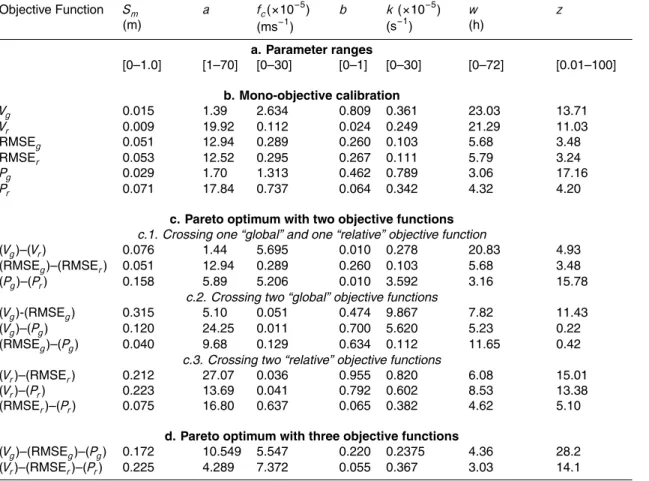
Table 1. Parameter ranges applied for the diff_{erent automatic calibration together with the}

mono-objective calibration and the balanced multi-objective Pareto optimum solution.

Objective Function Sm

(m)

a fc(×10−5)

(ms−1)

b k(×10−5)

(s−1)

w (h)

z

a. Parameter ranges

[0–1.0] [1–70] [0–30] [0–1] [0–30] [0–72] [0.01–100]

b. Mono-objective calibration

Vg 0.015 1.39 2.634 0.809 0.361 23.03 13.71

Vr 0.009 19.92 0.112 0.024 0.249 21.29 11.03

RMSEg 0.051 12.94 0.289 0.260 0.103 5.68 3.48

RMSE_r 0.053 12.52 0.295 0.267 0.111 5.79 3.24

Pg 0.029 1.70 1.313 0.462 0.789 3.06 17.16

Pr 0.071 17.84 0.737 0.064 0.342 4.32 4.20

c. Pareto optimum with two objective functions c.1. Crossing one “global” and one “relative” objective function

(Vg)–(Vr) 0.076 1.44 5.695 0.010 0.278 20.83 4.93

(RMSE_g)–(RMSE_r) 0.051 12.94 0.289 0.260 0.103 5.68 3.48

(P_g)–(P_r) 0.158 5.89 5.206 0.010 3.592 3.16 15.78

c.2. Crossing two “global” objective functions

(Vg)-(RMSEg) 0.315 5.10 0.051 0.474 9.867 7.82 11.43

(V_g)–(P_g) 0.120 24.25 0.011 0.700 5.620 5.23 0.22

(RMSEg)–(Pg) 0.040 9.68 0.129 0.634 0.112 11.65 0.42

c.3. Crossing two “relative” objective functions

(Vr)–(RMSEr) 0.212 27.07 0.036 0.955 0.820 6.08 15.01

(V_r)–(P_r) 0.223 13.69 0.041 0.792 0.602 8.53 13.38

(RMSE_r)–(Pr) 0.075 16.80 0.637 0.065 0.382 4.62 5.10

d. Pareto optimum with three objective functions

(V_g)–(RMSE_g)–(P_g) 0.172 10.549 5.547 0.220 0.2375 4.36 28.2

(28)

HESSD

4, 1031–1067, 2007

Title Page

Tables Figures

◭ ◮

Back Close

Full Screen / Esc

Table 2.Values of the three objective functionsV_r, RMSE_randP_rwhen using the calibrated

pa-rameters with the mono-objective calibration and the balanced two-objective or three-objective Pareto optimum solution.

Objective function Criteria value used for calibration

V_r[–] RMSE_r(m3s−1) P_r[–] Mono-objective (V_r) 0.087 43.2 0.278 Mono-objective (RMSE_r) 0.158 26.0 0.159 Mono-objective (P_r) 0.191 32.4 0.134 Two-objective (V_r)–(RMSE_r) 0.117 33.4 0.216 Two-objective (V_r)–(P_r) 0.116 34.4 0.197 Two-objective (RMSE_r)–(P_r) 0.180 29.4 0.145 Three-objective (V_r)–(RMSE_r)–(P_r) 0.126 33.3 0.214

(29)

HESSD

4, 1031–1067, 2007

Title Page

Tables Figures

◭ ◮

Back Close

Full Screen / Esc

Table 3. Meansε_V andε_Qof the relative prediction error on runoff_{depth and peakflow of the}

calibration and validation events when using the calibrated parameters with the mono-objective calibration and the balanced two-objective or three-objective Pareto optimum solution.

Objective function Runoff_depth_ε

V PeakflowεQ

used for calibration

(30)