www.atmos-chem-phys.net/16/4213/2016/ doi:10.5194/acp-16-4213-2016
© Author(s) 2016. CC Attribution 3.0 License.
Potential sensitivity of photosynthesis and isoprene emission to
direct radiative effects of atmospheric aerosol pollution
Susanna Strada1,aand Nadine Unger1
1School of Forestry and Environmental Studies, Yale University, New Haven, CT, USA anow at: Laboratoire des Sciences du Climat et de l’Environnement, Gif-sur-Yvette, France
Correspondence to: Susanna Strada ([email protected])
Received: 16 July 2015 – Published in Atmos. Chem. Phys. Discuss.: 17 September 2015 Revised: 13 February 2016 – Accepted: 15 March 2016 – Published: 4 April 2016
Abstract. A global Earth system model is applied to quan-tify the impacts of direct anthropogenic aerosol effective ra-diative forcing on gross primary productivity (GPP) and iso-prene emission. The impacts of different pollution aerosol sources (anthropogenic, biomass burning, and non-biomass burning) are investigated by performing sensitivity experi-ments. The model framework includes all known light and meteorological responses of photosynthesis, but uses fixed canopy structures and phenology. On a global scale, our re-sults show that global land carbon fluxes (GPP and isoprene emission) are not sensitive to pollution aerosols, even under a global decline in surface solar radiation (direct+diffuse) by ∼9 %. At a regional scale, GPP and isoprene emis-sion show a robust but opposite sensitivity to pollution aerosols in regions where forested canopies dominate. In eastern North America and Eurasia, anthropogenic pollu-tion aerosols (mainly from non-biomass burning sources) en-hance GPP by +5–8 % on an annual average. In the north-western Amazon Basin and central Africa, biomass burning aerosols increase GPP by+2–5 % on an annual average, with a peak in the northwestern Amazon Basin during the dry-fire season (+5–8 %). The prevailing mechanism varies across regions: light scattering dominates in eastern North Amer-ica, while a reduction in direct radiation dominates in Europe and China. Aerosol-induced GPP productivity increases in the Amazon and central Africa include an additional positive feedback from reduced canopy temperatures in response to increases in canopy conductance. In Eurasia and northeast-ern China, anthropogenic pollution aerosols drive a decrease in isoprene emission of−2 to−12 % on an annual average. Future research needs to incorporate the indirect effects of
aerosols and possible feedbacks from dynamic carbon allo-cation and phenology.
1 Introduction
Terrestrial gross primary productivity (GPP), the amount of carbon dioxide (CO2) taken up every year from the atmo-sphere by plant photosynthesis, is the largest single flux in the carbon cycle and therefore plays a major role in global climate change. GPP is closely connected with climatic vari-ables (e.g., temperature, water, light) (Beer et al., 2010). In turn, terrestrial vegetation provides the main source of isoprene to the atmosphere, which controls the loading of multiple short-lived climate pollutants and greenhouse gases (ozone, methane, secondary aerosols). Isoprene production is closely linked to plant photosynthesis (Pacifico et al., 2009; Unger et al., 2013). Hence, both GPP and isoprene emis-sion may be influenced by a change in surface solar radiation (SSR, the sum of the direct and diffuse radiation incident on the surface) and surface atmospheric temperature (SAT). An-thropogenic aerosols affect directly the Earth’s radiation flux via (a) scattering, which alters the partitioning between direct and diffuse radiation, increases the diffuse fraction of SSR, and affects SAT (Wild, 2009); and (b) absorption, which re-duces SSR and SAT (Ramanathan et al., 2001). Furthermore, aerosols may attenuate indirectly SSR by acting as cloud condensation nuclei, thus perturbing cloud cover and cloud properties (Rosenfeld et al., 2008).
im-pacts on climate, and on the water and carbon cycles (Jones and Cox, 2001; Gu et al., 2003; Trenberth and Dai, 2007). In the aftermath of the eruption, a loss in net global radiation at the TOA (top of the atmosphere) and a concomitant cooling were observed, and ultimately led to drying (Trenberth and Dai, 2007). By efficiently scattering light, the volcanic sul-fate aerosol production caused a significant increase in dif-fuse solar radiation. In 1991 and 1992, at two northern mid-latitude sites, Molineaux and Ineichen (1996) recorded an in-crease in clear-sky diffuse radiation by+50 %, compensated for by a concomitant decrease in direct radiation of−30 %. Over the same period, in a deciduous forest in North Amer-ica, Gu et al. (2003) ascribed to increased diffuse radiation an enhancement in plant productivity of+23 and+8 % in the 2 years following the Pinatubo eruption. On the global scale, enhancement in the terrestrial carbon sink was proposed as one of the main drivers of the sharp and rapid decline in the rate of atmospheric CO2 rise observed in the post-Pinatubo period, which resulted in a decrease of 3.5 ppmv by 1995 in atmospheric CO2 (Keeling et al., 1995; Jones and Cox, 2001; Gu et al., 2003). The “Mount Pinatubo experiment” suggested a possible global response of terrestrial vegetation to the “diffuse fertilization effect” (DFE). Observational and theoretical studies show that plant productivity is more ef-ficient under multi-directional diffuse rather than direct light because shaded non-light-saturated leaves increase their pho-tosynthetic rate (Gu et al., 2002).
The DFE on plant photosynthesis has been extensively ob-served at ecosystem scale under cloudy skies (e.g., Gu et al., 2002; Niyogi et al., 2004; Cheng et al., 2015) and a chronic aerosol loading (e.g., Gu et al., 2003; Oliveira et al., 2007; Cirino et al., 2014) in diverse ecosystems (rainforest, decid-uous and needleleaf forest, croplands and grasslands). The main conclusions of these studies are the following: (1) DFE prevails in complex and closed canopies, such as forests (Niyogi et al., 2004; Kanniah et al., 2012); and (2) intermedi-ate aerosol optical depth (AOD) enhances plant productivity, while high AOD (>2–3) reduces the carbon uptake rate be-cause of a large reduction in direct radiation (Oliveira et al., 2007; Artaxo et al., 2013; Cirino et al., 2014). An ecosystem-scale measurement study in a European mixed needleleaf and deciduous forest reported increased isoprene emissions un-der conditions of higher diffuse light (Laffineur et al., 2013). A few modeling studies have investigated aerosol-induced effects on plant productivity. Regional- and daily-scale as-sessments have been performed over the Yellow River region (China), selecting a period of 5 days (Steiner and Chamei-des, 2005), and over the eastern United States, selecting two growing seasons (Matsui et al., 2008). Results in both studies are consistent with the main conclusions of the local obser-vational studies. Steiner and Chameides (2005) demonstrated the importance of both aerosol-induced radiative (i.e., change in light amount and its partitioning) and thermal (i.e., change in surface temperature) effects on plant transpiration and pro-ductivity. However, these studies focus on short time
peri-ods and a limited number of ecosystems using offline models with single-layer canopy schemes.
By applying a multi-layer canopy scheme in an of-fline modeling framework (i.e., aerosol, radiative transfer, and land-surface models are coupled offline), Rap et al. (2015) performed a regional- and decadal-scale assessment of aerosol-induced effects on plant productivity in the Ama-zon Basin from 1998 to 2007. The authors specifically fo-cused on biomass burning aerosols (BBAs) and assessed the fact that BBAs increase the annual mean diffuse light and net primary production (NPP) by, respectively,∼5 and∼2.5 %. Deforestation fires play a key role and drive∼40 % of the es-timated changes in light and photosynthesis. Moreover, Rap et al. (2015) assessed that in the Amazon Basin during 1998– 2007 the DFE (a) was larger than the CO2fertilization effect, and (b) it could counteract the negative effect of droughts on land carbon fluxes.
A global-scale assessment of the aerosol-induced effects on the carbon cycle was performed by Mercado et al. (2009) using an offline land-surface model with a multi-layer canopy scheme. The authors concluded that DFE en-hanced the global land carbon sink by+23.7 % over the 20th century, under an overall radiation (direct+diffuse) change of +9.3 %. Mercado et al. (2009) reconstructed historical SSR using radiative transfer calculations and a global cli-mate data set for the “global dimming” (period 1950–1980) and the “global brightening” period (after the 1990s) (Wild, 2009, 2012; Streets et al., 2009). Recently, Chen and Zhuang (2014) applied an atmospheric radiative transfer module cou-pled with a terrestrial ecosystem model to quantify aerosol direct radiative effects on global terrestrial carbon dynam-ics during 2003–2010. Using transient atmospheric CO2and the prognostic leaf area index (LAI, one-sided green leaf area per unit ground area), the authors evaluated aerosol im-pacts on plant phenology, thermal and hydrological condi-tions, as well as solar radiation. Chen and Zhuang (2014) estimated that, on a global scale, aerosols enhance GPP by 4.9 Pg C yr−1 and slightly affect respiration. Chen and Zhuang (2014) accounted for all atmospheric aerosols and they did not target anthropogenic pollution aerosols.
focuses on GPP because it is the first step in the long-term storage of atmospheric CO2 in the living tissues of plants and is directly affected by solar radiation. We do not address aerosol effects on other land carbon cycle fluxes (e.g., respi-ration, net ecosystem exchange). We employ the effective ra-diative forcing (ERF) concept metric introduced in the IPCC AR5 in which all physical variables are allowed to respond to the direct aerosol–radiation perturbations except for those concerning the ocean and sea ice (Myhre et al., 2013b). The inclusion of these rapid adjustments in the ERF metric allows us to investigate the multiple aerosol-induced concomitant meteorological impacts on the biosphere.
Section 2 describes the global Earth system model tool (NASA ModelE2-YIBs) and the experimental design. In Sect. 3, we evaluate simulated present-day atmospheric aerosols and GPP against global observational data sets in-cluding AOD from the Moderate Resolution Imaging Spec-troradiometer (MODIS) and global gridded GPP that was generated using data-orientated diagnostic upscaling of site-derived GPP from FLUXNET (Beer et al., 2010; Bonan et al., 2011; Jung et al., 2011). In addition, we present the analysis of results from the sensitivity simulations. In Sect. 4, we discuss the results and summarize conclusions.
2 Methodology
2.1 Global Earth system model: NASA ModelE2-YIBs We apply the NASA GISS ModelE2 global chemistry– climate model at 2◦×2.5◦ latitude by longitude horizon-tal resolution with 40 vertical layers extending to 0.1 hPa (Schmidt et al., 2014). The Yale Interactive Terrestrial Bio-sphere Model (YIBs) is embedded inside NASA ModelE2 in a framework known as NASA ModelE2-YIBs (Unger et al., 2013). The global climate model provides the meteorolog-ical drivers for the vegetation physiology. The land-surface hydrology submodel provides the grid-cell-level soil charac-teristics to the vegetation physiology. The model framework fully integrates the land biosphere–oxidant–aerosol system such that these components interact with each other and with the physics of the climate model. Online oxidants affect aerosol production and online aerosols provide surfaces for chemical reactions and influence photolysis rates. The chem-istry and aerosol schemes and their coupling have been well documented and extensively compared with observations and other global models (e.g., Bell et al., 2005; Bauer et al., 2007; Koch et al., 2006; Koch and Del Genio, 2010; Unger, 2011; Myhre et al., 2013a; Shindell et al., 2006, 2013a, b; Steven-son et al., 2013).
The aerosol package includes mass-based simulation of sulfate, nitrate and sea salt (e.g., Koch et al., 2006), car-bonaceous aerosols (black carbon, BC, and primary organic matter, OC) (Koch and Hansen, 2005), mineral dust (Miller et al., 2006), and biogenic secondary organic aerosol (BSOA) (Tsigaridis and Kanakidou, 2007). The model assumes
log-normal size distributions with effective radii: 0.2 µm (sul-fate); 0.3 µm (nitrate); 0.1 µm (BC); 0.3 µm (OC). Sea salt aerosols are represented by two size bins with effective radii of 0.44 and 5 µm. Mineral dust aerosols are tracked in four size bins, ranging from 0.1 to 10 µm, and can be coated by sulfate and nitrate aerosols. Hygroscopic aerosols (sulfates, nitrates, sea salt, and organic carbon) increase in size with in-creasing relative humidity, which increases the aerosol scat-tering efficiency and radiative forcing (Schmidt et al., 2006). The direct effect interaction between aerosols and radia-tion is reproduced by the online (two-way coupled) mode: aerosol fields are simulated at each model time step (30 min) and influence the simulated shortwave and longwave radia-tion through scattering and absorpradia-tion in the radiaradia-tion sub-model, which in turn influences the climate dynamics. Thus, aerosols induce (a) changes in simulated diffuse and direct photosynthetically active radiation (PAR, spectral range of surface visible solar radiation, 400–700 nm, used by plants to photosynthesize) that are passed from the radiation submodel to the vegetation model; and (b) rapid adjustment changes in meteorology (temperature, precipitation, circulation) that are passed from the model’s atmosphere and land surface to the vegetation model.
2.1.1 The Yale Interactive Terrestrial Biosphere model (YIBs)
The vegetation structure describes eight plant functional types (PFTs): tundra, grassland, shrubland, deciduous broadleaf forest, savannah, tropical rainforest, evergreen needleleaf forest, and cropland. The PFT-specific vegeta-tion cover fracvegeta-tion and LAI are the standard atlas-based dis-tribution in NASA GISS ModelE2 (Schmidt et al., 2014). The LAI for each PFT is prescribed according to regu-lar seasonal sinusoidal variation between PFT-specific min-imum and maxmin-imum seasonal LAI values that is insensi-tive to climate drivers or carbon balances (Rosenzweig and Abramopoulos, 1997; Friend and Kiang, 2005). Each model PFT fraction in the vegetated part of each grid cell repre-sents a single canopy. The canopy radiative transfer scheme assumes a closed canopy and divides vertical canopy lay-ers into sunlit and shaded leaves, as well as the different contributions from direct and diffuse PAR (from the climate model’s radiation scheme) at the leaf level (Spitters et al., 1986). The leaf-level carbon and water fluxes are scaled up to the canopy level by integrating over each canopy layer, using an adaptive number of layers (typically 2–16) (Friend and Kiang, 2005). After upscaling from leaf to canopy, the carbon and water fluxes are exchanged with the atmosphere on the 30 min physical integration time step of the global cli-mate model.
1987). In the leaf model, the rate of net CO2uptake in the leaves of C3plants is the result of three competing processes: Jc, the carboxylation-limited rate;Je, the electron transport-limited photosynthesis rate; and Js, the export-limited rate to use photosynthesis products. The coupled photosynthesis, stomatal conductance, and diffusive CO2flux transport equa-tions are solved analytically at the leaf level using a cubic function in the net carbon assimilation rate. Isoprene emis-sion is calculated as a function ofJe, intercellular and atmo-spheric CO2, and canopy temperature (Unger et al., 2013).
As theoretical and observational studies have demon-strated, the aerosol effect on plant photosynthesis strongly depends on the canopy separation into sunlit and shaded leaves. These two parts of the canopy have different re-sponses to the change in light partitioning driven by aerosols (Knohl and Baldocchi, 2008). Under low PAR, both shaded and sunlit leaves are in a light-limited environment (Je con-trols the photosynthesis rate). Under high PAR, sunlit leaves are light-saturated and in a Rubisco-limited environment (Jc controls the photosynthesis rate), while shaded leaves are in a light-limited environment (Je). Hence, sunlit canopy pho-tosynthesis depends on both direct and diffuse light, and on both Jc andJe photosynthesis rates, while shaded canopy photosynthesis is directly influenced by diffuse light and mainly depends on the Je photosynthesis rate. The aerosol light-scattering directly influences Je; hence, it mainly af-fects shaded leaves (Matsui et al., 2008; Chen and Zhuang, 2014).
Linkages between vegetation and atmospheric aerosols are extremely complex. This version of the land carbon cycle model captures the meteorological (light, temperature, rel-ative humidity, precipitation) responses of photosynthesis. The use of fixed canopy structures and phenology means that leaf mass is not driven by photosynthetic uptake of CO2 and a closed carbon cycle is not simulated. Thus, the sim-ulated GPP and isoprene emission responses may be under-estimated because the LAI is insensitive to CO2uptake and climate. The objectives here are to examine the meteorolog-ical responses in detail and to offer a benchmark for future research that will incorporate additional feedbacks from dy-namic LAI and phenology. For example, aerosol-induced ef-fects on light and surface temperature may alter (i) the onset and shutdown dates of photosynthesis and growing season length (Yue et al., 2015a) and (ii) the carbon allocation, LAI, and tree height that provide a feedback to GPP (Yue et al., 2015b).
2.2 Simulations
The atmosphere-only configuration of NASA ModelE2-YIBs is used to perform a control simulation (SimC-TRL) representative of the present-day (∼2000 s). Pre-scribed decadal average monthly varying sea surface tem-perature (SST) and sea ice observations for 1996–2005 from the HadSST data set (Rayner et al., 2006) provide the
lower boundary conditions for the global climate model. The present-day trace gas and aerosol emissions are pre-scribed to year 2000 values from the historical inventory developed for IPCC AR5 (Lamarque et al., 2010). At-mospheric levels of long-lived greenhouse gases are pre-scribed to CO2=370 ppmv, CH4=1733 ppbv in the South-ern Hemisphere, and 1814 ppbv in the NorthSouth-ern Hemisphere; N2O=316 ppbv. A set of three sensitivity perturbation sim-ulations is performed that selectively removes anthropogenic short-lived gas-phase precursor and primary aerosol emis-sions:
a. all anthropogenic emissions, including biomass burn-ing, are removed in SimNOant;
b. only biomass burning emissions are removed in Sim-NObb;
c. all industrial emissions, which means all anthropogenic emissions except biomass burning emissions (e.g., in-dustry, power generation, road vehicles; hereafter, we refer to these emissions as “non-biomass burning emis-sions”), are removed in SimNOind.
The control and sensitivity simulations are run for 32 model years recycling the year 2000 boundary conditions every year but allowing the changes in atmospheric aerosol composition to influence meteorology and the land bio-sphere. By prescribing SSTs and sea ice cover at climato-logical values, while letting all other physical components of the Earth system respond until they reach steady state, we capture the short-term response of the land-surface cli-mate to the aerosol radiation perturbation. This fixed-SST technique allows us to compute ERF, the forcing metric that accounts for rapid tropospheric adjustments and better char-acterizes drivers in the troposphere (e.g., aerosols) (Myhre et al., 2013b). Hence, the fixed-SST technique enables us to analyze multiple meteorological effects of the direct aerosol– radiation interactions. The long run time is necessary to allow the fast land and atmosphere climatic feedbacks to respond to the aerosol perturbations and the TOA radiation fluxes to equilibrate. Integrations of 32 model years are completed for all simulations (control and sensitivity runs). The global at-mospheric oxidant–aerosol composition usually takes about 2 years to spin up, while the atmospheric dynamics and land-surface climate takes about 10 years to reach steady state due to an imposed aerosol radiative forcing. Therefore, we dis-card the first 12 model run years as spin-up. The remain-ing 20 model run years are averaged for analysis. Twenty model years of data are necessary such that any aerosol-driven variable differences between the control and sensitiv-ity simulations are statistically significant relative to internal climate model variability. Our goal is to isolate the effects of aerosol pollution on the land biospheric fluxes. Therefore, we compute the absolute differences inXvariable as1X=
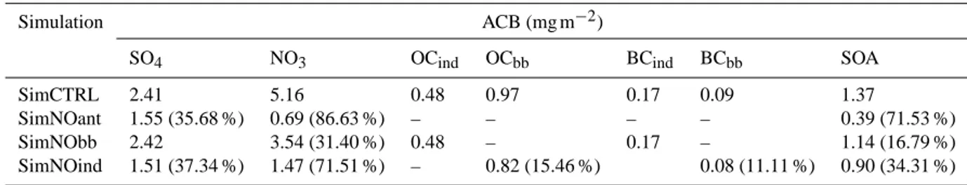
Table 1. Global annual average of aerosol column burden (ACB, mg m−2) as simulated by NASA ModelE2-YIBs in the control and sensi-tivity present-day simulations for, in order, sulfates, nitrates, organic (OC) and black carbon (BC) from industrial (ind) and biomass burning (bb), and secondary organic aerosols (SOA). Cases filled with “–” refer to negligible values of ACB (i.e., order of magnitude pg m−2). For sensitivity simulations, percentage values in parentheses indicate the contribution of target emissions (i.e., anthropogenic, biomass burning, and non-biomass burning) to each aerosol component.
Simulation ACB (mg m−2)
SO4 NO3 OCind OCbb BCind BCbb SOA
SimCTRL 2.41 5.16 0.48 0.97 0.17 0.09 1.37
SimNOant 1.55 (35.68 %) 0.69 (86.63 %) – – – – 0.39 (71.53 %)
SimNObb 2.42 3.54 (31.40 %) 0.48 – 0.17 – 1.14 (16.79 %)
SimNOind 1.51 (37.34 %) 1.47 (71.51 %) – 0.82 (15.46 %) 0.08 (11.11 %) 0.90 (34.31 %)
Table 2. Global annual average of effective radiative forcing (ERF) for aerosol–radiation interactions (W m−2) as simulated by NASA ModelE2-YIBs in present-day simulations for, in order, sulfates, nitrates, organic (OC) and black carbon (BC) from industrial (ind) and biomass burning (bb), and secondary organic aerosols (SOA). The global annual average ERF is calculated as the difference between the control experiment (SimCTRL) and sensitivity experiments: SimNOant, without all anthropogenic emissions; SimNObb, without biomass burning emissions; and SimNOind, without anthropogenic emissions except biomass burning. Percentage values in parentheses specify the contribution of target emissions (i.e., anthropogenic, biomass burning, and non-biomass burning) to the ERF of the selected aerosol component. The abbreviation “ns” indicates differences that are not statistically significant at the 95 % confidence level (based on a Student’s
ttest).
Species ERF (W m−2)
SimCTRL−SimNOant SimCTRL−SimNObb SimCTRL−SimNOind
SO4 −0.31 (40.17 %) ns −0.30 (39.75 %)
NO3 −0.38 (85.09 %) −0.14 (30.38 %) −0.31 (69.80 %)
OCind −0.06 (100.00 %) ns −0.06 (100.00 %)
OCbb −0.11 (100.00 %) −0.11 (100.00 %) −0.01 (9.43 %)
BCind 0.18 (100.00 %) ns 0.18 (100.00 %)
BCbb 0.12 (100.00 %) 0.12 (100.00 %) 0.02 (11.42 %) SOA 0.10 (63.48 %) −0.03 (15.86 %) −0.05 (29.27 %)
and, for selected variables, are gathered in the Supplement. Applying the same methodology, we compute absolute and percentage differences in annual and seasonal averages over selected regions. Hereafter, we define as “significant” all ab-solute/percentage changes that are statistically significant at the 95 % confidence level.
3 Results
3.1 Evaluation of present-day control simulation Present-day values of the global mean aerosol column bur-den (ACB) and ERF for aerosol–radiation interactions (i.e., aerosol direct effect) are presented by component in Tables 1 and 2. The IPCC AR5 provides RF (not ERF) by single aerosol species (Boucher et al., 2013; Myhre et al., 2013b). NASA ModelE2-YIBs ERF values for single aerosol species are consistent with the AR5 RF ranges. Nitrate ERF is on the lower bound of the AR5 RF range (−0.30 to−0.03 W m−2). ERFs of sulfate, BC from industrial sources, and SOAs fall into the AR5 RF ranges (respectively, −0.60 to−0.20,
+0.05 to+0.80, and−0.27 to−0.20 W m−2). OC from in-dustrial sources and BBAs show ERFs consistent with the AR5 RF values (OCind:−0.09 W m−2; BBAs: 0.00 W m−2). Based on a combination of methods (i.e., global aerosol mod-els and observation-based methods), the AR5 report esti-mates the total ERF due to aerosol–radiation interactions:
−0.45 (−0.95 to+0.05) W m−2; in AR5, the best total RF estimate of the aerosol–radiation interaction is−0.35 (−0.85 to+0.15) W m−2 (Myhre et al., 2013b). The total ERF is computed in NASA ModelE2-YIBs as the arithmetic mean of all anthropogenic aerosol components (i.e., sulfate, ni-trate, OC, and BC from both industrial and biomass burn-ing sources, SOA, and dust). The NASA ModelE2-YIBs es-timates a total ERF due to aerosol–radiation interactions of
−0.34 (−0.76 to+0.18) W m−2, at the low end of the IPCC AR5 range.
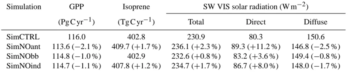
understand-Table 3. Global annual average gross primary productivity (GPP), isoprene emission, and shortwave visible (SW VIS) total, direct, and dif-fuse solar radiation as simulated by NASA ModelE2-YIBs in the control and sensitivity present-day simulations. For sensitivity simulations, percentage changes compared to the control simulation are indicated in parentheses and reported only if changes are statistically significant at the 95 % confidence level.
Simulation GPP Isoprene SW VIS solar radiation (W m−2)
(Pg C yr−1) (Tg C yr−1) Total Direct Diffuse
SimCTRL 116.0 402.8 230.9 80.3 150.6
SimNOant 113.6 (−2.1 %) 409.7 (+1.7 %) 236.1 (+2.3 %) 89.3 (+11.2 %) 146.8 (−2.5 %) SimNObb 114.8 (−1.0 %) 402.9 232.6 (+0.8 %) 83.2 (+3.6 %) 149.4 (−0.8 %) SimNOind 114.7 (−1.1 %) 407.8 (+1.2 %) 234.7 (+1.7 %) 86.7 (+8.0 %) 148.0 (−1.7 %)
Table 4. Linear correlation Pearson’s coefficient (Pearson’s R), Pearson’sR squared (R2), and root-mean-squared error (RMSE) as computed for model evaluation for annual and seasonal average coarse aerosol optical depth (AOD) and gross primary productiv-ity (GPP). Performances of the NASA ModelE2-YIBs in the con-trol present-day simulation (∼ 2000s) are compared to (1) MODIS AOD (at 550 nm; averaged over 2000–2007) for NASA ModelE2-YIBs PM10 optical depth and the (2) global FLUXNET-derived GPP product (averaged over 2000–2011). Only boreal summer (JJA) and winter (DJF) seasonal averages are reported.
Variable Average Pearson’sR R2 RMSE
AOD Annual 0.679 0.461 0.054
JJA 0.769 0.591 0.064
DJF 0.591 0.349 0.065
GPP Annual 0.863 0.745 1.025
JJA 0.782 0.611 1.796
DJF 0.899 0.808 1.137
ing of the present-day carbon cycle budget (based on FLUXNET: 123±8 Pg C yr−1, Beer et al., 2010; based on MODIS: 109.29 Pg C yr−1, Zhao et al., 2005; based on the Eddy Covariance-Light Use Efficiency model: 110.5±
21.3 Pg C yr−1, Yuan et al., 2010). The global isoprene source is 402.8 Tg C yr−1, which is at the low end of the range of previous global estimates (e.g., 400–700 Tg C yr−1, Guenther et al., 2006). However, a recent study suggests a larger range of 250–600 Tg C yr−1(Messina et al., 2015). The photosynthesis-based isoprene emission models tend to esti-mate a lower global isoprene source than empirical models because the scheme intrinsically accounts for the effects of plant water availability that reduce isoprene emission rates (Unger et al., 2013).
3.1.1 Aerosol optical depth (AOD)
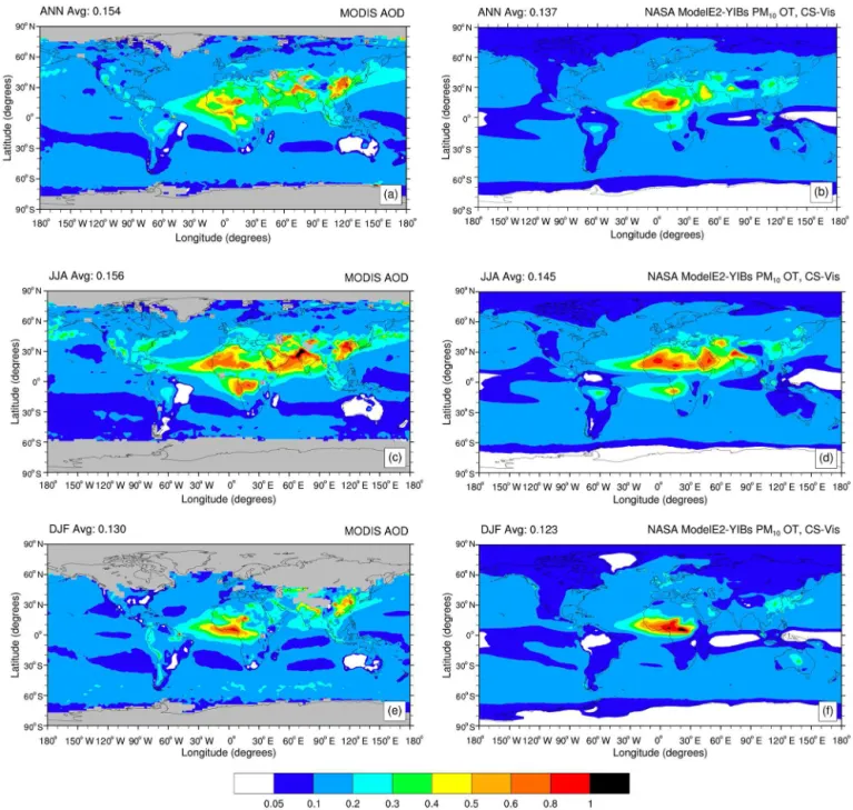
We use the quality assured Terra MODIS Collection 5 (C5.1) monthly mean product (Level 3), a globally gridded data set at 1◦×1◦ resolution re-gridded to 2◦×2.5◦ resolution for comparison with the global model. To infer clear-sky (non-cloudy) aerosol properties in part of the visible and
short-wave infrared spectrum, MODIS C5.1 relies on two algo-rithms depending on surface reflectance: (1) the Dark Target (DT) algorithm, under conditions of low surface reflectance (e.g., over ocean, vegetation) (Levy et al., 2010); and (2) the Deep Blue (DB) algorithm, designed to work under high sur-face reflectance, such as over desert regions (Hsu et al., 2004; Shi et al., 2014). To cover both dark and bright surfaces, we merge the DT and DB AOD products (i.e., DT missing data are filled in with DB values). We use MODIS TERRA C5.1 AOD data from 2000 to 2007 because DB AOD data are only available for this period due to calibration issues (Shi et al., 2014). The MODIS instrument also measures the fine model weighting (ETA) at 550 nm; consequently, the fine-mode AOD can be computed as fine AOD=AOD×ETA, where fine AOD is the fraction of the AOD contributed by fine-mode sized particles (i.e., effective radius≪1.0 µm) (Levy et al., 2010; Bian et al., 2010). Quantitative use of MODIS fine AOD is not appropriate because fine-mode aerosols play a main role in the scattering process (Levy et al., 2010).
NASA ModelE2-YIBs provides separately all-sky and clear-sky AOD diagnostics; we focus on clear-sky output since that is more comparable to the spaceborne observa-tions. The model coarse-mode (PM10, atmospheric particu-late matter with diameter< 10 µm) AOD includes all simu-lated aerosol species (sulfate, nitrate, organic and black car-bon, SOA, sea salt, and mineral dust); the model fine-mode (PM2.5, atmospheric PM with diameter< 2.5 µm) AOD ac-counts for all simulated aerosol species except sea salt and dust.
Figure 1. Annual and seasonal average coarse aerosol optical depth (AOD) seen by (a, c, e) the MODIS instrument (at 550 nm; averaged over 2000–2007) and (b, d, f) NASA ModelE2-YIBs in the control present-day simulation (∼ 2000 s). Global mean values are given in the upper left corner of each map. Only boreal summer (JJA) and winter (DJF) seasonal averages are shown. For NASA ModelE2-YIBs, only clear-sky (CS) values in the visible (Vis) range are used to define PM10optical thickness (OT).
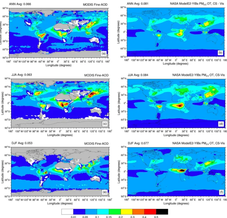
the impacts of anthropogenic pollution aerosols on the land carbon fluxes. The spatial and temporal distribution of fine-mode aerosols in NASA ModelE2-YIBs is consistent with MODIS observations (Fig. 2). In general, the model shows a slightly higher fine-aerosol layer compared to MODIS (e.g., over Europe, India, and South America). Over China, model fine-AOD distribution is consistent with MODIS on the annual average; however, the model does not show the seasonal variability that MODIS observes. To quantify the
model evaluation, on an annual average the NASA ModelE2-YIBs coarse-mode AOD global means present an accept-able correlation with the MODIS AOD global means (R =
recom-Figure 2. As Fig. 1 for fine-mode aerosol optical depth: (a, c, e) MODIS fine AOD and (b, d, f) model PM2.5OT.
mended, we do not quantify model performance for fine-mode AODs.
3.1.2 Gross primary productivity (GPP)
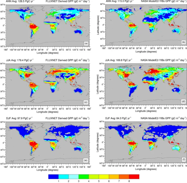
In Fig. 3, we compare the spatial distribution of annual and seasonal (boreal summer and winter) mean GPP in the NASA ModelE2-YIBs model (control present-day simula-tion) with a global FLUXNET-derived GPP product (aver-aged over 2000–2011). The model is consistent with the broad spatio-temporal variability in FLUXNET-derived GPP. We find a weaker annual and seasonal signal in the model
GPP over the cerrado area in central South America. How-ever, since the FLUXNET-derived GPP product mainly re-lies on the availability of FLUXNET sites, which are densely distributed in temperate zones not in the tropics, FLUXNET-derived GPP may be biased over central South America. On an annual average, the NASA ModelE2-YIBs GPP highly correlates with the FLUXNET-derived GPP (R = 0.9,R2=
Figure 3. Annual and seasonal average gross primary productivity (GPP, in g m−2day−1) as seen by (a, c, e) a global FLUXNET-derived GPP product (averaged over 2000–2011), and (b, d, f) NASA ModelE2-YIBS in the control present-day simulation (∼ 2000s). Global mean values are given in the upper left corner of each map. Only boreal summer (JJA) and winter (DJF) seasonal averages are shown.
the YIBs model over 145 sites for different PFTs. Depending on PFT, GPP simulation biases range from−19 to+7 %. For monthly average GPP, among the 145 sites, 121 have corre-lations higher than 0.8. High correcorre-lations (>0.8) are mainly achieved at deciduous broadleaf and evergreen needle leaf sites; crop sites show medium correlation (∼0.7).
3.2 Aerosol pollution changes in sensitivity simulations 3.2.1 Global scale
0.99 mg m−2 to SOA ACB (72 %). Biomass burning emis-sions (SimCTRL−SimNObb) contribute 1.62 mg m−2to ni-trate ACB (31 %) and 0.23 mg m−2 to SOA ACB (17 %), while they do not significantly contribute to sulfate ACB. Non-biomass burning emissions (SimCTRL−SimNOind) contribute 0.89 mg m−2to sulfate ACB (37 %), 3.69 mg m−2 to nitrate ACB (72 %), and 0.47 mg m−2 to SOA ACB (34 %). For carbonaceous aerosols, anthropogenic pollu-tion emissions contribute 1.45 mg m−2 to the total OC ACB (0.48 mg m−2 from non-biomass burning, OCind, and 0.97 mg m−2from biomass burning, OCbb) and 0.26 mg m−2 to the total BC ACB (0.17 mg m−2from non-biomass burn-ing, BCind, and 0.09 mg m−2from biomass burning, BCbb). Non-biomass burning emissions contribute 0.15 mg m−2 to OCbbACB (15 %) and 0.01 mg m−2to BCbbACB (15 %).
Table 2 presents, by aerosol component, the ERF for aerosol–radiation interactions due to anthropogenic pollution and biomass burning and non-biomass burning emissions. Anthropogenic pollution emissions contribute−0.31 W m−2 to sulfate ERF (40 % of the total sulfate ERF due to both anthropogenic and natural emissions), −0.38 W m−2 to ni-trate ERF (85 %), and +0.10 W m−2 to SOA ERF (63 %). Biomass burning emissions contribute −0.14 W m−2 to ni-trate ERF (30 %) and −0.03 W m−2 to SOA ERF (16 %), while they do not significantly contribute to sulfate ERF. Non-biomass burning emissions contribute−0.30 W m−2to sulfate ERF (40 %), −0.31 W m−2 to nitrate ERF (70 %), and −0.05 W m−2 to SOA ERF (29 %). For carbona-ceous aerosols, anthropogenic pollution emissions con-tribute −0.17 W m−2 to the total OC ERF (−0.06 W m−2 from non-biomass burning, OCind, and−0.11 W m−2 from biomass burning, OCbb) and +0.30 W m−2 to the total BC ERF (+0.18 W m−2 from non-biomass burning, BC
ind, and +0.12 W m−2 from biomass burning, BCbb). Non-biomass burning emissions contribute −0.01 W m−2 to OCbb ERF (9 %) and+0.02 W m−2to BCbbERF (11 %).
3.2.2 Five key regions
Beyond the global results, our simulations reveal five strongly sensitive regions that correspond to important sources of aerosol pollution: eastern North America, Eura-sia, northeastern China, the northwestern Amazon Basin, and central Africa (green boxes in Fig. 4). Besides a substan-tial contribution to primary aerosol (PA) sources (i.e., BC and OC), all selected regions considerably contribute to sec-ondary aerosol (SA) sources such as sulfate, nitrate, and SOA (Table S1 for ACB and Table S2 for ERF in the Supplement). We focus on SAs since, being finer than PAs, they play a key role in scattering and may trigger DFE.
In terms of aerosol burden, in the five key regions, ni-trate is the dominant aerosol source, with a larger contribu-tion from non-biomass burning compared to biomass burn-ing emissions. Sulfate source is mainly governed by non-biomass burning emissions, except in central Africa, where
biomass burning emissions importantly contribute to sulfate ACB. For SOA sources, both biomass and non-biomass burn-ing emissions feed SOA ACB, with a larger contribution from biomass burning in central Africa.
Eastern North America and Eurasia share a similar contri-bution to nitrate ACB (∼14–15 mg m−2;∼93 %) and ERF (−1.2–1.3 mg m−2; ∼94 %) due to anthropogenic emis-sions, with the largest input from non-biomass burning emissions (ACB: 12.7 mg m−2; ERF:−1.1 mg m−2,∼80 %) compared to biomass burning emissions (ACB: 3.4 mg m−2; ERF: −0.3 mg m−2, ∼20 %). Eastern North America and Eurasia also show a similar contribution to SOA sources due to anthropogenic emissions (ACB: 2.1 mg m−2,∼78 %; ERF:−0.2 mg m−2,∼72 %). In both regions, non-biomass burning emissions provide a larger input to SOA sources compared to biomass burning emissions, with a larger con-tribution in Eurasia compared to eastern North America (ACB: 1.4 vs. 0.9 mg m−2, 52 vs. 32 %) and even a dif-ferent sign in ERF (−0.2 vs.+0.08 mg m−2, 45 vs. 25 %). Compared to eastern North America and Eurasia, northeast-ern China presents nearly a half nitrate source, while contri-butions to sulfate ACB due to anthropogenic emissions are about 0.5–1 W m−2 (5–10 %) larger, and lead to more in-tense negative ERF (by 0.4–0.6 W m−2, 5–10 %). In north-eastern China, anthropogenic emissions largely contribute as well to SOA sources, with a share between biomass and non-biomass burning similar to Eurasia. The northwestern Ama-zon Basin shows the smallest contributions to SA sources. However, compared to the other key regions, biomass burn-ing and non-biomass burnburn-ing emissions contribute the same amount to SOA sources (ACB: 0.5 W m−2, 24–29 %; ERF: −0.06 W m−2, 24–29 %). As previously commented, central Africa substantially contributes to sulfate source via both biomass (ACB: 0.6 W m−2, 30 %; ERF:−0.2 W m−2, 30 %) and non-biomass burning emissions (ACB: 0.7 W m−2, 40 %; ERF:−0.3 W m−2, 45 %). In this region, biomass burning emissions substantially feed SOA sources, with contributions that nearly double those from non-biomass burning emis-sions (ACB: 2.1 vs. 1.1 W m−2, 44 vs. 22 %; ERF: −0.16 vs.−0.08 W m−2, 48 vs. 23 %).
3.3 Aerosol pollution changes to surface solar radiation 3.3.1 Global scale
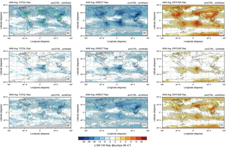
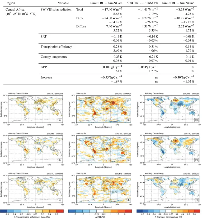
radi-Figure 4. Spatial distribution of annual absolute change in shortwave visible (SW VIS) (a, d, g) total, (b, e, h) direct, and (c, f, i) diffuse solar radiation (in W m−2). Changes are computed between the control experiment (SimCTRL) and sensitivity experiments: (a–c) without all anthropogenic emissions (SimNOant); (d–f) without biomass burning emissions (SimNObb); and (g–i) without anthropogenic emissions except biomass burning (SimNOind). All experiments are set in a present-day climatic state. Shaded regions indicate areas where changes in solar radiation are significant at the 95 % confidence level. Green boxes on plot (a) highlight key regions selected for discussion.
ation show a larger sensitivity range to the aerosol bur-den (absolute change: 2.9–8.9 W m−2; relative change: 3.6– 11.2 %). In the present-day world, anthropogenic pollution aerosols drive a decrease in global total and direct radia-tion by −2.3 % (−5.2 W m−2) and−11.2 % (−9.0 W m−2), respectively, while global diffuse radiation increases by
+2.5 % (+3.7 W m−2). Biomass burning aerosols have al-most zero effect on global total and diffuse radiation, while they reduce direct radiation by−3.6 % (−2.9 W m−2). Non-biomass burning aerosols (non-BBAs) decrease global to-tal radiation by −1.7 % (−3.8 W m−2) and increase global diffuse radiation by the same percentage (absolute change:
+2.6 W m−2), while global direct radiation decreases by
−8.0 % (−6.4 W m−2). In summary, anthropogenic pollution aerosols drive an overall SSR (direct+diffuse) global de-cline of∼5 W m−2. In the literature, estimates for the over-all SSR decline during the “global dimming” (period 1950– 1980) range from 3 to 9 W m−2(Wild, 2012). In percentage, anthropogenic pollution aerosols drive an overall SSR global decline of 8.7 %.
3.3.2 Five key regions
Figure 4 shows the spatial distribution of aerosol-driven an-nual absolute changes in surface radiation (for anan-nual per-centage and seasonal absolute changes: Figs. S1 and S2). Regionally, on both annual and seasonal average, eastern North America, Eurasia, northeastern China, the northwest-ern Amazon Basin and central Africa are highly affected by aerosol-induced changes in surface solar radiation. For these five key regions, Table 5 presents absolute and percent changes in annual average radiation (total, direct, and dif-fuse) between the control and sensitivity simulations. Eastern North America shows the largest increase in annual diffuse radiation due to all anthropogenic aerosols (+8.6 W m−2;
+6.2 %), followed by northeastern China and central Africa, which experience similar changes (∼ +7.4–7.9 W m−2; ∼ +5.7 %). Over eastern North America, the increase in diffuse radiation maximizes during boreal summer (+13.6 W m−2;
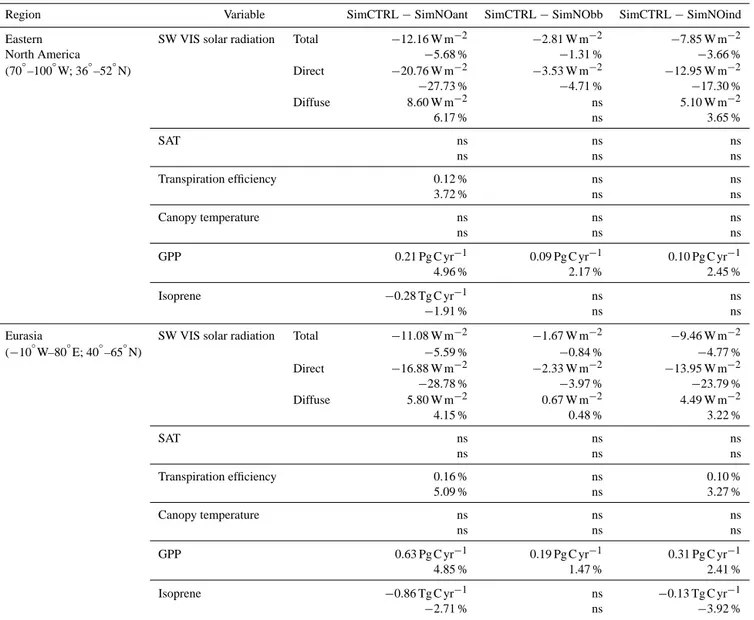
Eura-Table 5. Absolute and percent changes in annual average shortwave visible (SW VIS) solar radiation, surface atmospheric temperature (SAT), transpiration efficiency, canopy temperature, gross primary productivity (GPP), and isoprene emission in eastern North America, Eurasia, northeastern China, the northwestern Amazon Basin, and central Africa (green boxes in Fig. 4a). Changes are computed between the control experiment (SimCTRL) and sensitivity experiments: SimNOant, without all anthropogenic emissions; SimNObb, without biomass burning emissions; and SimNOind, without anthropogenic emissions except biomass burning. The abbreviation “ns” indicates differences that are not statistically significant at the 95 % confidence level (based on a Student’sttest).
Region Variable SimCTRL−SimNOant SimCTRL−SimNObb SimCTRL−SimNOind
Eastern SW VIS solar radiation Total −12.16 W m−2 −2.81 W m−2 −7.85 W m−2
North America −5.68 % −1.31 % −3.66 %
(70◦–100◦W; 36◦–52◦N) Direct −20.76 W m−2 −3.53 W m−2 −12.95 W m−2
−27.73 % −4.71 % −17.30 %
Diffuse 8.60 W m−2 ns 5.10 W m−2
6.17 % ns 3.65 %
SAT ns ns ns
ns ns ns
Transpiration efficiency 0.12 % ns ns
3.72 % ns ns
Canopy temperature ns ns ns
ns ns ns
GPP 0.21 Pg C yr−1 0.09 Pg C yr−1 0.10 Pg C yr−1
4.96 % 2.17 % 2.45 %
Isoprene −0.28 Tg C yr−1 ns ns
−1.91 % ns ns
Eurasia SW VIS solar radiation Total −11.08 W m−2 −1.67 W m−2 −9.46 W m−2
(−10◦W–80◦E; 40◦–65◦N) −5.59 % −0.84 % −4.77 %
Direct −16.88 W m−2 −2.33 W m−2 −13.95 W m−2
−28.78 % −3.97 % −23.79 %
Diffuse 5.80 W m−2 0.67 W m−2 4.49 W m−2
4.15 % 0.48 % 3.22 %
SAT ns ns ns
ns ns ns
Transpiration efficiency 0.16 % ns 0.10 %
5.09 % ns 3.27 %
Canopy temperature ns ns ns
ns ns ns
GPP 0.63 Pg C yr−1 0.19 Pg C yr−1 0.31 Pg C yr−1
4.85 % 1.47 % 2.41 %
Isoprene −0.86 Tg C yr−1 ns −0.13 Tg C yr−1
−2.71 % ns −3.92 %
sia (Table S3). Driven by non-BBAs, Eurasia and northeast-ern China undergo the largest reduction in total and direct ra-diation, with a larger increase over northeastern China (total:
−12.3 W m−2, −6 %; direct:−19.4 W m−2, −26.1 %) than Eurasia (total: −9.5 W m−2, −4.8 %; direct: −14 W m−2,
−23.8 %). Over Eurasia and northeastern China, decreases in total and direct radiation maximize during boreal summer, with changes that double those observed over eastern North America (Table S3). In central Africa and the northeastern Amazon, on an annual average basis, BBAs drive changes in surface radiation that are similar in magnitude to those driven by non-BBAs. However, in these tropical ecosystems, the BBA effects on surface radiation exhibit a strong seasonal
cycle, with the maximum signal in the dry-fire season (boreal summer–boreal autumn, JJA–SON).
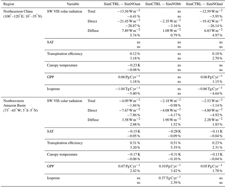
Table 5. Continued.
Region Variable SimCTRL−SimNOant SimCTRL−SimNObb SimCTRL−SimNOind
Northeastern China SW VIS solar radiation Total −13.56 W m−2 ns −12.59 W m−2
(100◦–120◦E; 10◦–35◦N) −6.41 % ns −5.95 %
Direct −21.45 W m−2 −2.35 W m−2 −19.42 W m−2
−28.87 % −3.16 % −26.14 %
Diffuse 7.89 W m−2 1.08 W m−2 6.83 W m−2
5.74 % 0.79 % 4.97 %
SAT ns ns ns
ns ns ns
Transpiration efficiency 0.12 % ns 0.10 %
3.18 % ns 2.70 %
Canopy temperature −0.23 K ns ns
−0.08 % ns ns
GPP 0.06 Pg C yr−1 ns 0.06 Pg C yr−1
1.18 % ns 1.15 %
Isoprene −1.04 Tg C yr−1 ns −0.86 Tg C yr−1
−5.60 % ns −4.64 %
Northwestern SW VIS solar radiation Total −4.09 W m−2 −2.18 W m−2 −2.52 W m−2
Amazon Basin −1.84 % −0.98 % −1.14 %
(73◦–65◦W; 5◦S–5◦N) Direct −7.67 W m−2 −4.08 W m−2 −4.80 W m−2
−7.86 % −4.17 % −4.92 %
Diffuse 3.58 W m−2 1.90 W m−2 2.28 W m−2
2.88 % 1.52 % 1.83 %
SAT −0.15 K −0.28 K −0.11 K
−0.05 % −0.09 % −0.04 %
Transpiration efficiency 0.31 % 0.51 % 0.23 %
3.20 % 5.19 % 2.31 %
Canopy temperature −0.17 K −0.31 K −0.13 K
−0.06 % −0.10 % −0.04 %
GPP 0.07 Pg C yr−1 0.10 Pg C yr−1 0.05 Pg C yr−1
2.42 % 3.42 % 1.78 %
Isoprene ns 0.37 Tg C yr−1 ns
ns 2.39 % ns
3.4 Aerosol pollution changes to surface meteorology Accounting for only the direct aerosol effect and using the fixed-SST technique, we limit the influence of pollution aerosols on the Earth system to direct changes in surface ra-diation that affect the atmosphere and land surface only. For this reason, in the following we mainly relate changes in land carbon fluxes to changes in surface radiation, surface meteo-rology (e.g., SAT and relative humidity), and plant conditions (e.g., transpiration, canopy temperature).
The radiation changes caused by anthropogenic aerosol pollution do not exert a statistically significant change in global and annual average SAT because our experiments use fixed SSTs and do not consider aerosol indirect effects on clouds. The rapid adjustments are allowed for the atmosphere and land surface only. For the same reasons, we do not find statistically significant changes in precipitation or in cloud water content due to anthropogenic aerosol pollution (not
shown). The model does simulate statistically robust changes in annual average SAT in the two tropical key regions: the northwestern Amazon Basin and central Africa (Fig. S3 in the Supplement). From the sensitivity experiments, we as-certain that the SAT changes are associated with the BBAs in the tropical regions (Fig. S3 and Table S4). The mechanism occurs through a bio-meteorological feedback described be-low.
Table 5. Continued.
Region Variable SimCTRL−SimNOant SimCTRL−SimNObb SimCTRL−SimNOind
Central Africa SW VIS solar radiation Total −17.40 W m−2 −14.41 W m−2 −8.53 W m−2
(10◦–25◦E; 10◦S–5◦N) −8.68 % −7.19 % −4.25 %
Direct −24.80 W m−2 −18.72 W m−2 −10.75 W m−2
−34.85 % −26.32 % −15.12 %
Diffuse 7.40 W m−2 4.31 W m−2 2.22 W m−2
5.72 % 3.33 % 1.72 %
SAT −0.19 K −0.16 K −0.08 K
−0.06 % −0.05 % −0.03 %
Transpiration efficiency 0.28 % 0.31 % 0.14 %
3.60 % 4.06 % 1.79 %
Canopy temperature −0.23 K −0.21 K −0.11 K
−0.08 % −0.07 % −0.04 %
GPP 0.10 Pg C yr−1 0.08 Pg C yr−1 ns
1.61 % 1.27 % ns
Isoprene −0.55 Tg C yr−1 ns −0.30 Tg C yr−1
−1.89 % ns −1.02 %
with increases in canopy conductance and relative humid-ity (RH) via increased transpiration. Under anthropogenic aerosol pollution, transpiration efficiency shows significant modifications in all five key regions (Fig. 5 and Table 5). The northwestern Amazon Basin records the largest absolute in-crease in transpiration efficiency due to BBAs (∼0.51; per-centage change: ∼5 %). Among industrialized regions, the largest absolute increases in transpiration efficiency are ob-served in Eurasia due to all anthropogenic aerosols (0.16; percentage change: ∼5 %), one-third of the increases in transpiration efficiency observed in the northwestern Ama-zon Basin. Among the five key regions, changes in canopy temperature are statistically robust only in the northwestern Amazon Basin, central Africa, and northeastern China. The northwestern Amazon Basin experiences the largest decrease in canopy temperature driven by BBAs (−0.31 K;−0.10 %), which is∼0.1 K larger than the decrease in canopy temper-ature over central Africa and northeastern China. Due to an-thropogenic pollution aerosols, central Africa and northeast-ern China experience a similar decrease in canopy tempera-ture (−0.23 K;−0.08 %), and, compared to the northwestern Amazon Basin, they undergo substantial decreases in direct radiation (−35 % in central Africa and−29 % in northeastern China vs.−8 % in the northwestern Amazon Basin).
To summarize, in the model, reductions in the canopy tem-perature observed in the northwestern Amazon Basin rep-resent a positive feedback on plant productivity (further in-creases) in response to the DRF-driven increases. In indus-trial key regions such as eastern North America and Eurasia, changes in the quantity and quality of surface solar radiation play the main role in affecting plant photosynthesis. In north-eastern China and central Africa, multiple aerosol-driven ef-fects may combine to affect plant photosynthesis: changes in the quantity and quality of surface solar radiation (as in east-ern North America and Eurasia) and reductions in the canopy temperature (as in the northwestern Amazon Basin).
3.5 Sensitivity of GPP to aerosol pollution 3.5.1 Global scale
Changes in the global annual average GPP flux between the control and the sensitivity simulations are reported in Ta-ble 3. Global GPP shows a weak sensitivity to pollution aerosols (∼1–2 %). Global GPP is increased by up to 2.0 % (2.4 Pg C yr−1) at most due to all anthropogenic aerosol pol-lution. Biomass burning and non-biomass burning aerosols have a comparable effect on global GPP. In contrast to Mer-cado et al. (2009), our model results do not suggest a sub-stantial change in global GPP due to pollution aerosols.
3.5.2 Five key regions
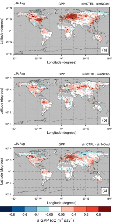
Anthropogenic aerosol pollution drives regional increases in annual average plant productivity (GPP) that affect the five key regions (Fig. 6 and, for percentage changes, Fig. S6). The strongest increases in GPP occur in eastern North Amer-ica and Eurasia (+0.2–0.3 g C m−2day−1;+5–8 %) (Figs. 6a and S7a). In the northwestern Amazon Basin, BBAs drive similar absolute increases in GPP (+0.2–0.3 g C m−2day−1;
+2–5 %) (Figs. 6b and S7b).
Anthropogenic aerosols drive the strongest absolute en-hancement in GPP in Eurasia (+0.62 Pg C yr−1;∼5 %), fol-lowed by eastern North America, which experiences a third of the absolute increase in GPP but similar relative increases (+0.21 Pg C yr−1; ∼5 %) (Table 5). In northeastern China, anthropogenic aerosols drive the lowest enhancement in GPP, which is one-tenth of the absolute increases in GPP observed in Eurasia (+0.06 Pg C yr−1; 1.2 %; Table 5). The northwest-ern Amazon Basin and central Africa record increases in GPP that are slightly stronger than those observed in north-eastern China (+0.07–0.10 Pg C yr−1; 1.6–2.4 %; Table 5).
In each key region, increases in GPP are governed by dif-ferent aerosol types. In the industrial key regions, non-BBAs play a key role in GPP enhancement, while, in biomass burn-ing regions (i.e., the northwestern Amazon Basin and cen-tral Africa), BBAs govern GPP enhancement. In northeast-ern China, BBAs do not drive any robust change in GPP; in Eurasia, BBAs drive increases in GPP, that is, two-thirds of the increases due to non-BBAs (+0.2 vs.+0.3 Pg C yr−1; 1.5 vs. 2.4 %) (Table 5). In eastern North America, BBAs and non-BBAs contribute a similar amount to GPP enhancement (+0.1 Pg C yr−1, ∼2 %; Table 5). In central Africa, BBAs entirely control increases in GPP, whereas, in the northwest-ern Amazon Basin, BBAs drive increases in GPP larger than the increase due to all anthropogenic aerosols and non-BBAs (+0.1 Pg C yr−1, 3.4 %; Table 5).
During boreal summer, anthropogenic aerosol pollution increases GPP in eastern North America and Eurasia by up to
+5–8 %, 0.6–0.8 g C m−2day−1(Figs. 7a and S7c); particu-larly, in Eurasia aerosol pollution from non-BBAs drives the increase in GPP (Figs. 6c and S7f). Driven by BBAs in the dry-fire season, GPP increases by+0.05–0.4 g C m−2day−1 (+2–5 %) in eastern Europe (boreal evergreen and mixed forests), and by +0.4–0.6 g C m−2day−1 (+5–8 %) in the northwestern Amazon Basin (Figs. 7b and S7e).
During boreal summer, Eurasia shows the largest abso-lute enhancement in GPP (+1.8 Pg C yr−1; +6 %), mainly driven by non-BBAs (+1.1 Pg C yr−1;+3.4 %) compared to BBAs (+0.5 Pg C yr−1;+1.5 %). The absolute GPP increase in eastern North America is one-third of that observed in Eurasia (+0.5 Pg C yr−1; +6 %) (Table S3). In the north-western Amazon Basin, the largest enhancement in GPP oc-curs during boreal autumn driven by BBAs (+0.2 Pg C yr−1;
radi-Figure 6. Spatial distribution of annual absolute change in gross primary productivity (GPP, in g C m−2day−1) between the control experiment (SimCTRL) and sensitivity experiments: (a) without all anthropogenic emissions (SimNOant); (b) without biomass burn-ing emissions (SimNObb); and (c) without anthropogenic emissions except biomass burning (SimNOind). All experiments are set in a present-day climatic state. Shaded regions indicate areas where changes in GPP are significant at the 95 % confidence level. Green boxes on plot (a) highlight key regions selected for discussion.
ations maximize during boreal summer (Table S3). Like-wise, in central Africa, changes in surface radiations peak during boreal summer, while the largest enhancements in GPP (and decreases in canopy temperature) occur during
bo-Figure 7. As Fig. 6 for seasonal (boreal summer, JJA) absolute change in gross primary productivity (GPP, in g C m−2day−1) be-tween the control experiment (SimCTRL) and sensitivity experi-ments: (a) SimNOant, (b) SimNObb, and (c) SimNOind.
The GPP sensitivities to aerosol pollution in the five key regions presented in this work agree well with val-ues from previous measurement-based and modeling stud-ies (e.g., Niyogi et al., 2004; Steiner and Chameides, 2005; Knohl and Baldocchi, 2008; Matsui et al., 2008). Consistent with previous measurement-based studies, pollution aerosols have the largest impacts on GPP for these PFTs with com-plex canopy architectures (e.g., Niyogi et al., 2004; Alton et al., 2007; Cirino et al., 2014). For instance, the five key regions are all populated by PFTs with multi-layer canopies, large canopy heights and LAIs, such as deciduous broadleaf forests, evergreen needleleaf forests, mixed forests, and trop-ical rainforests, which happen to be co-located with high sources of anthropogenic aerosol pollution. In the Amazon Basin, previous studies measured enhancement in CO2 up-take at ecosystem scale during the biomass burning season; these observationally based studies attributed the rise in CO2 uptake to the increase in diffuse light, although substantial changes in surface temperature and humidity were also mea-sured (e.g., Oliveira et al., 2007; Doughty et al., 2010; Cirino et al., 2014). Using a modeling framework, Rap et al. (2015) estimated that BBAs enhance GPP by 0.7–1.6 %, for an in-crease in diffuse radiation of 3.4–6.8 %. Their estimated GPP sensitivity for this region is lower than values presented here because Rap et al. (2015) did not account for aerosol-induced reductions in leaf temperature.
Anthropogenic aerosol pollution substantially enhances plant productivity at a regional scale. This analysis suggests that aerosol-driven enhancements in GPP result from differ-ent mechanisms that depend on region. In the model, light scattering and DRF dominate in eastern North America, re-duction in direct radiation dominates in Eurasia and north-eastern China, and tropical ecosystems (i.e., the northwest-ern Amazon Basin and central Africa) benefit from a bio-meteorological feedback to canopy temperature.
3.6 Sensitivity of isoprene emission to aerosol pollution 3.6.1 Global scale
Changes in the global annual average isoprene emission be-tween the control and the sensitivity simulations are reported in Table 3. Similar to GPP, global isoprene emission shows a weak sensitivity to pollution aerosols (∼1–2 %). Global iso-prene emission decreases by up to 1.7 % (6.9 Pg C yr−1) for SimNOant. Global isoprene emissions are sensitive to indus-trial emissions but not to biomass burning emissions.
3.6.2 Five key regions
Anthropogenic aerosol pollution drives a decrease in annual average isoprene emission of −0.5 to −1 mg C m−2day−1 (−2 to−12 %) over Europe and China (Figs. 8 and S7). Non-biomass burning sources are mainly responsible for the ob-served regional decrease in annual average isoprene
sion. In peak growing season in the temperate and trop-ical zone, pollution aerosols do not affect isoprene emis-sion (Fig. S8). On an annual average basis, anthropogenic aerosols mainly from non-biomass burning sources (i.e., BBAs have no robust effect) drive the largest decreases in isoprene source over northeastern China (−1.04 Tg C yr−1;
−5.6 %) and Eurasia (−0.86 Tg C yr−1;−2.7 %) (Table 5). In response to aerosol pollution from non-biomass burn-ing sources, Europe and China show a large decrease in an-nual average direct radiation (−24–26 %) but a similar in-crease in diffuse radiation (+3–5 %) to eastern North Amer-ica (Table 5). Hence, over Europe and China, aerosol-driven reduction in direct light is not adequately sustained by an increase in diffuse radiation, which limits isoprene emis-sion, due to the reduced light supply (reduced Je). Thus, in Europe and China, we find that aerosol-induced reduc-tion in direct radiareduc-tion drives isoprene decreases and con-comitant GPP increases. Even when photosynthesis is light-saturated (in a Rubisco-limited environment), isoprene emis-sion continues to rise under increasing PAR (Morfopoulos et al., 2013). This divergent response has been observed at the ecosystem scale (Sharkey and Loreto, 1993). At 20◦C and at any photon flux, the authors recorded nearly no isoprene emission; at 30◦C, isoprene emission increased with photon flux up to 1600 µmol m−2s−1, while photosynthesis was al-ready saturated; at 40◦C, isoprene emission maximized at 1000 µmol m−2s−1; afterwards, it decreased when the pho-ton flux was raised to 1600 µmol m−2s−1.
In the northwestern Amazon Basin, annual average iso-prene emission increases are simulated in response to BBAs (+0.4 Tg C yr−1;+2.4 %) (Table 5), although the area of sta-tistical significance is small. In this region, the influence of increases in GPP on isoprene emission overrides the influ-ence of the cooler canopy temperatures (Table 5).
4 Discussion and conclusions
Aerosol-induced effects on land carbon fluxes (GPP and iso-prene emission) were investigated using a coupled global vegetation–chemistry–climate model. By performing sensi-tivity experiments, we isolated the role of pollution aerosol sources (anthropogenic, biomass burning, and non-biomass burning). Our results suggest that global-scale land car-bon fluxes (GPP and isoprene emission) are not sensitive to pollution aerosols, even under a robust overall SSR (di-rect+diffuse) global change (∼9 %). We found substantial but divergent sensitivities of GPP and isoprene emission to pollution aerosols at a regional scale. In eastern North Amer-ica and Eurasia, anthropogenic pollution aerosols (mainly from non-biomass burning sources) enhance GPP by +5– 8 % on an annual average. In the northwestern Amazon Basin and central Africa, biomass burning aerosols increase GPP by+2–5 % on an annual average (+5–8 % at the peak of the dry-fire season in the northwestern Amazon Basin). In Eura-sia and northeastern China, anthropogenic pollution aerosols
(mainly from non-biomass burning sources) drive a decrease in isoprene emission of−2 to−12 % on annual average. Our model results imply that reductions of anthropogenic pollu-tion aerosols over Europe and China below the present-day loadings may trigger an enhancement in isoprene emission, with consequences for ozone and aerosol air quality.
We acknowledge three main limitations. Firstly, we tack-led the direct aerosol effects only and did not consider first and second indirect effects of aerosols such that we are partly missing the impact of aerosol–cloud interactions on land carbon fluxes. Secondly, we used the fixed SST technique; hence, we accounted only for rapid adjustments of land-surface climate to aerosol radiation perturbation. Thirdly, we did not include feedbacks from dynamic LAI and phenology that may lead to an underestimation of the effects of aerosol-induced effects on plant productivity. Future research will address these three limitations. Future changes in regional atmospheric aerosol loadings will have substantial implica-tions for the regional land carbon cycle.
The Supplement related to this article is available online at doi:10.5194/acp-16-4213-2016-supplement.
Author contributions. S. Strada and N. Unger designed the experi-ments. S. Strada performed the simulations. S. Strada and N. Unger prepared the manuscript.
Acknowledgements. This project was supported in part by the facilities and staff of the Yale University Faculty of Arts and Sciences High Performance Computing Center.
Edited by: D. Spracklen
References
Alton, P. B., North, P. R., and Los, S. O.: The impact of diffuse sun-light on canopy sun-light-use efficiency, gross photosynthetic prod-uct and net ecosystem exchange in three forest biomes, Global Change Biol., 13, 776–787, 2007.
Arneth, A., Monson, R. K., Schurgers, G., Niinemets, Ü., and Palmer, P. I.: Why are estimates of global terrestrial isoprene emissions so similar (and why is this not so for monoterpenes)?, Atmos. Chem. Phys., 8, 4605–4620, doi:10.5194/acp-8-4605-2008, 2008.
Artaxo, P., Rizzo, L. V., Brito, J. F., Barbosa, H. M. J., Arana, A., Sena, E. T., Cirino, G. G., Bastos, W., Martin, S. T., and An-dreae, M. O.: Atmospheric aerosols in Amazonia and land use change: from natural biogenic to biomass burning conditions, Faraday Discuss., 165, 203–235, doi:10.1039/C3FD00052D, 2013.
Ball, J. T., Woodrow, I. E., and Berry, J. A.: A model predicting stomatal conductance and its contribution to the control of photo-synthesis under different environmental conditions, in: Progress in Photosynthesis Research, edited by: Biggins, J., Nijhoff, Dor-drecht, the Netherlands, 221–224, 1987
Bauer, S. E., Koch, D., Unger, N., Metzger, S. M., Shindell, D. T., and Streets, D. G.: Nitrate aerosols today and in 2030: a global simulation including aerosols and tropospheric ozone, At-mos. Chem. Phys., 7, 5043–5059, doi:10.5194/acp-7-5043-2007, 2007.
Beer, C., Reichstein, M., Tomelleri, E., Ciais, P., Jung, M., Car-valhais, N., Rödenbeck, C., Arain, M. A., Baldocchi, D., Bo-nan, G. B., Bondeau, A., Cescatti, A., Lasslop, G., Lindroth, A., Lomas, M., Luyssaert, S., Margolis, H., Oleson, K. W., Roup-sard, O., Veenendaal, E., Viovy, N., Williams, C., Wood-ward, F. I., and Papale, D.: Terrestrial gross carbon dioxide up-take: global distribution and covariation with climate, Science, 329, 834–838, 2010.
Bell, N., Koch, D., and Shindell, D.: Impacts of chemistry-aerosol coupling on tropospheric ozone and sulfate simulations in a general circulation model, J. Geophys. Res.-Atmos., 110, D14, doi:10.1029/2004JD005538, 2005.
Bian, H., Chin, M., Kawa, S. R., Yu, H., Diehl, T., and Kuc-sera, T.: Multiscale carbon monoxide and aerosol correlations from satellite measurements and the GOCART model: implica-tion for emissions and atmospheric evoluimplica-tion, J. Geophys. Res.-Atmos., 115, D07302, doi:10.1029/2009JD012781, 2010. Bonan, G. B., Lawrence, P. J., Oleson, K. W., Levis, S., Jung, M.,
Reichstein, M., Lawrence, D., and Swenson, S. C.: Improv-ing canopy processes in the Community Land Model ver-sion 4 (CLM4) using global flux fields empirically inferred from FLUXNET data, J. Geophys. Res.-Biogeo., 116, G2, doi:10.1029/2010JG001593, 2011.
Boucher, O., Randall, D., Artaxo, P., Bretherton, C., Feingold, G., Forster, P., Kerminen, V.-M., Kondo, Y., Liao, H., Lohmann, U., Rasch, P., Satheesh, S. K., Sherwood, S., Stevens, B., and Zhang, X. Y.: Clouds and Aerosols, in: Climate Change 2013: The Physical Science Basis, Contribution of Working Group I to the Fifth Assessment Report of the Intergovernmental Panel on Climate Change, Cambridge University Press, Cambridge, UK and New York, NY, USA, 571–656, 2013.
Carlton, A. G., Pinder, R. W., Bhave, P. V., and Pouliot, G. A.: To what extent can biogenic SOA be controlled?, Environ. Sci. Technol., 44, 3376–3380, 2010.
Chen, M. and Zhuang, Q.: Evaluating aerosol direct radiative effects on global terrestrial ecosystem carbon dynamics from 2003 to 2010, Tellus B, 66, 21808, doi:10.3402/tellusb.v66.21808, 2014. Cheng, S. J., Bohrer, G., Steiner, A. L., Hollinger, D. Y., Suyker, A., Phillips, P. R., and Nadelhoffer, K. J.: Variations in the influ-ence of diffuse light on gross primary productivity in temperate ecosystems, Agr. Forest Meteorol., 201, 98–110, 2015.
Cirino, G. G., Souza, R. A. F., Adams, D. K., and Artaxo, P.: The ef-fect of atmospheric aerosol particles and clouds on net ecosystem
exchange in the Amazon, Atmos. Chem. Phys., 14, 6523–6543, doi:10.5194/acp-14-6523-2014, 2014.
Doughty, C. E., Flanner, M. G., and Goulden, M. L.: Effect of smoke on subcanopy shaded light, canopy temperature, and carbon dioxide uptake in an Amazon rainforest, Global Bio-geochem. Cy., 24, GB3015, doi:10.1029/2009GB003670, 2010. Farquhar, G. D., von Caemmerer, S. V., and Berry, J. A.: A bio-chemical model of photosynthetic CO2assimilation in leaves of C3species, Planta, 149, 78–90, 1980.
Ford, B. and Heald, C. L.: Aerosol loading in the Southeastern United States: reconciling surface and satellite observations, At-mos. Chem. Phys., 13, 9269–9283, doi:10.5194/acp-13-9269-2013, 2013.
Forster, P., Ramaswamy, V., Artaxo, P., Berntsen, T., Betts, R., Fa-hey, D. W., Haywood, J., Lean, J., Lowe, D. C., Myhre, G., Nganga, J., Prinn, R., Raga, G., Schulz, M. and Van Dorland, R.: Changes in Atmospheric Constituents and in Radiative Forcing, in: Climate Change 2007: The Physical Science Basis, Contribu-tion of Working Group I to the Fourth Assessment Report of the Intergovernmental Panel on Climate Change, Cambridge Univer-sity Press, Cambridge, UK and New York, NY, USA, 2007. Friend, A. D. and Kiang, N. Y.: Land surface model development
for the GISS GCM: effects of improved canopy physiology on simulated climate, J. Climate, 18, 2883–2902, 2005.
Gu, L., Baldocchi, D., Verma, S. B., Black, T., Vesala, T., Falge, E. M., and Dowty, P. R.: Advantages of diffuse radiation for terrestrial ecosystem productivity, J. Geophys. Res.-Atmos., 107, D6, doi:10.1029/2001JD001242, 2002.
Gu, L., Baldocchi, D. D., Wofsy, S. C., Munger, J. W., Michal-sky, J. J., Urbanski, S. P., and Boden, T. A.: Response of a de-ciduous forest to the Mount Pinatubo eruption: enhanced photo-synthesis, Science, 299, 2035–2038, 2003.
Guenther, A., Karl, T., Harley, P., Wiedinmyer, C., Palmer, P. I., and Geron, C.: Estimates of global terrestrial isoprene emissions using MEGAN (Model of Emissions of Gases and Aerosols from Nature), Atmos. Chem. Phys., 6, 3181–3210, doi:10.5194/acp-6-3181-2006, 2006.
Hsu, N. C., Tsay, S.-C., King, M., and Herman, J. R.: Aerosol prop-erties over bright-reflecting source regions, IEEE T. Geosci. Re-mote, 42, 557–569, 2004.
Jones, C. D. and Cox, P. M.: Modeling the volcanic signal in the atmospheric CO2record, Global Biogeochem. Cy., 15, 453–465, 2001.
Jung, M., Reichstein, M., Margolis, H. A., Cescatti, A., Richard-son, A. D., Arain, M. A., Arneth, A., Bernhofer, C., Bonal, D., Chen, J., Gianelle, D., Gobron, N., Kiely, G., Kutsch, W., Lass-lop, G., Law, B. E., Lindroth, A., Merbold, L., Montagnani, L., Moors, E. J., Papale, D., Sottocornola, M., Vaccari, F., and Williams, C.: Global patterns of land-atmosphere fluxes of car-bon dioxide, latent heat, and sensible heat derived from eddy co-variance, satellite, and meteorological observations, J. Geophys. Res.-Biogeo., 116, G3, doi:10.1029/2010JG001566, 2011. Kanniah, K. D., Beringer, J., North, P., and Hutley, L.: Control of
at-mospheric particles on diffuse radiation and terrestrial plant pro-ductivity: a review, Prog. Phys. Geogr., 36, 209–237, 2012. Keeling, C. D., Whorf, T. P., Wahlen, M., and Plicht, J. V. D.: