North Atlantic 20th century multidecadal variability in coupled climate models: sea surface temperature and ocean overturning circulation

(1)

OSD

8, 353–396, 2011

North Atlantic 20th century multidecadal

variability

I. Medhaug and T. Furevik

Title Page

Abstract Introduction

Conclusions References

Tables Figures

◭ ◮

Back Close

Full Screen / Esc

Printer-friendly Version Interactive Discussion

Discussion

P

a

per

|

Dis

cussion

P

a

per

|

Discussion

P

a

per

|

Discussio

n

P

a

per

|

Ocean Sci. Discuss., 8, 353–396, 2011 www.ocean-sci-discuss.net/8/353/2011/ doi:10.5194/osd-8-353-2011

Ocean Science Discussions

This discussion paper is/has been under review for the journal Ocean Science (OS). Please refer to the corresponding final paper in OS if available.

North Atlantic 20th century multidecadal

variability in coupled climate models: sea

surface temperature and ocean

overturning circulation

I. Medhaug and T. Furevik

Geophysical Institute and Bjerknes Centre for Climate Research, University of Bergen, Bergen, Norway

Received: 12 January 2011 – Accepted: 21 January 2011 – Published: 10 February 2011

Correspondence to: I. Medhaug (iselin.medhaug@gfi.uib.no)

(2)

OSD

8, 353–396, 2011

variability

Title Page

Tables Figures

◭ ◮

Back Close

Full Screen / Esc

Discussion

P

a

per

|

Dis

cussion

P

a

per

|

Discussion

P

a

per

|

Discussio

n

P

a

per

|

Abstract

Output from a total of 24 state-of-the-art Atmosphere-Ocean General Circulation Mod-els is analyzed. The modMod-els were integrated with observed forcing for the period 1850– 2000 as part of the Intergovernmental Panel on Climate Change (IPCC) Fourth Assess-ment Report. All models show enhanced variability at multi-decadal time scales in the 5

North Atlantic sector similar to the observations, but with a large intermodel spread in amplitudes and frequencies for both the Atlantic Multidecadal Oscillation (AMO) and the Atlantic Meridional Overturning Circulation (AMOC). The models, in general, are able to reproduce the observed geographical patterns of warm and cold episodes, but not the phasing such as the early warming (1930s–50s) and the following colder period 10

(1960s–80s). This indicates that the observed 20th century extreme in temperatures are due to primarily a fortuitous phasing of intrinsic climate variability and not domi-nated by external forcing. Most models show a realistic structure in the overturning circulation, where more than half of the available models have a mean overturning transport within the observed estimated range of 13–24 Sverdrup. Associated with a 15

stronger than normal AMOC, the surface temperature is increased and the sea ice ex-tent slightly reduced in the North Atlantic. Individual models show poex-tential for decadal prediction based on the relationship between the AMO and AMOC, but the models strongly disagree both in phasing and strength of the covariability. This makes it diffi -cult to identify common mechanisms and to assess the applicability for predictions. 20

1 Introduction

The ocean currents transport vast amounts of heat from low to high latitudes by the horizontal wind-driven gyre circulation and the density-driven thermohaline circulation (THC), with a maximum of_∼2 PW at 17◦_{N (Trenberth and Caron, 2001). In the}

At-lantic the THC component is known as the AtAt-lantic Meridional Overturning Circulation 25

(3)

OSD

8, 353–396, 2011

variability

Title Page

Tables Figures

◭ ◮

Back Close

Full Screen / Esc

Discussion

P

a

per

|

Dis

cussion

P

a

per

|

Discussion

P

a

per

|

Discussio

n

P

a

per

|

and saline water in the upper 1000 m, above a southward flowing colder and fresher water down to 3–4000 m. Below there is a deeper reversed cell of Antarctic bottom water (Delworth et al., 2008). The poleward transport of heat in the upper cell is an important driver for the climate system. At high latitudes the ocean is subjected to in-tense heat loss to the atmosphere and the water therefore loses buoyancy and sinks. 5

The potential energy lost in the sinking process is regained by wind- and tidal mixing across stable stratification further south, and the deep water gradually returns to the surface (Wunsch, 2002). On very long time scales (order of 1000 years) the AMOC is therefore sustained by mechanical energy input through wind- and tidal mixing.

Decadal to multidecadal variability in the North Atlantic climate has been found 10

in a large number of observational studies (e.g., Bjerknes, 1964; Kushnir, 1994; Schlesinger and Ramankutty, 1994; Delworth and Mann, 2000; Polyakov and Johnson, 2000), with two 20th century extremes being the early warming in the 1930s to 1950s, and the subsequent colder period during the 1960s to 1980s. From multimodel analysis of 20th century climate simulations, these temperature extremes have been attributed 15

mainly to the internal variability of the North Atlantic and not to the externally forced responses (Kravtsov and Spannagle, 2008; Knight, 2009; Ting et al., 2009). However, other model simulations indicate that both solar variability and volcanoes contribute in setting the phase of the variability (Hansen et al., 2005; Otter ˚a et al., 2010). The decadal to multidecadal temperature variations observed in the Nordic Seas and the 20

Arctic are seemingly related to the slowly varying SST field further to the south in the North Atlantic (Polyakov et al., 2004), where heat transport variability in both ocean and atmosphere appears to provide the link (e.g., Furevik, 2001). Bjerknes (1964) sug-gested that the decadal to multidecadal climate variations were driven by slow changes in the ocean gyre circulation, while many later studies indicate that the main cause is 25

(4)

OSD

8, 353–396, 2011

variability

Title Page

Tables Figures

◭ ◮

Back Close

Full Screen / Esc

Discussion

P

a

per

|

Dis

cussion

P

a

per

|

Discussion

P

a

per

|

Discussio

n

P

a

per

|

Knight et al., 2005), and the effect heat and salinity anomalies have on the density in the convective regions, and hence the strength of the deep water formation (e.g., Del-worth et al., 1993; Marshall et al., 2001; Bentsen et al., 2004; Jungclaus et al., 2005; Medhaug et al., 2011).

At present there is no consensus to what degree the AMOC variability is: a pure 5

ocean-only mode or a fully coupled atmosphere-ocean mode, with density fluctuations in the convection regions driven by advection of anomalous dense water from the south (e.g., Delworth et al., 1993; Vellinga and Wu, 2004); a fully coupled atmosphere-ocean or atmosphere-sea ice-ocean mode with the deep water formation rate dominated by variations in the local wind forcing (e.g., Dickson et al., 1996; Hkkinen, 1999; Eden and 10

Willebrand, 2001; Deshayes and Frankignoul, 2008; Msadek and Frankignoul, 2009; Medhaug et al., 2011); or if AMOC is simply a low frequency damped response to fluctuations in the atmospheric forcing fields (Hasselmann, 1976; Frankignoul et al., 1997; Frankcombe et al., 2009).

Low frequency variability in the ocean overturning circulation and possible relations 15

with upper ocean heat content and air-sea interaction of heat and moisture suggest a potential for predicting surface temperature and atmospheric mean state on annual to decadal time scales. Recent works in this rapidly growing research field suggest that AMOC is predictable up to 20 years (Collins et al., 2006). By relaxing the model to observed SSTs (Keenlyside et al., 2008), to upper ocean properties (temperature and 20

salinity) and atmospheric data (Smith et al., 2007), or to hydrographic observations (Pohlmann et al., 2009), the various groups have reported improved prediction skills of both global and regional climate. More precise understanding of the linkages between the hydrographic structure of the ocean, the large scale ocean circulation, and the impacts of variations in the ocean transports on atmospheric climate, will increase our 25

ability to give more realistic decadal forecasts in the years to come.

(5)

OSD

8, 353–396, 2011

variability

Title Page

Tables Figures

◭ ◮

Back Close

Full Screen / Esc

Discussion

P

a

per

|

Dis

cussion

P

a

per

|

Discussion

P

a

per

|

Discussio

n

P

a

per

|

measurements only available since 2004 (Cunningham et al., 2007). Due to the extent of the basin-scale circulation long term direct observations of the AMOC have not been conducted as it would require an unrealistic number of sections and instruments. As a result, neither the relationships between the AMO and AMOC in nature, nor the impacts of AMOC on North Atlantic climate variability are known. We therefore have to primarily 5

rely on models in this study.

For the first time the full range of Intergovernmental Panel on Climate Change (IPCC) Fourth Assessment Report (AR4) climate simulations for the 20th century integrations (1850–2000) have been used in a dedicated investigation of the connection between the two variables of North Atlantic multidecadal variability. Our main objectives have 10

been to investigate to what extent (i) the observed AMOC and AMO strength and vari-ability are captured in the climate models, (ii) relationships exist between the two mea-sures of multidecadal climate fluctuations, (iii) any physical mechanisms behind such relationships can be identified, and (iv) century long observations of SST can be used as a proxy for AMOC, and knowledge of the phase of the AMOC therefore will improve 15

our ability to predict climate on interannual to decadal time scales.

Section 2 gives an overview of the modelling and observational data sets used in this study and the applied statistical methods. The results of the model analysis, and comparison with observations, are given in Sect. 3, and the results and their implica-tions discussed in Sect. 4. Section 5 gives a summary with concluding remarks on the 20

implications for predictability of AMO and other climatic variables based on the state of the AMOC.

2 Methods and data 2.1 The coupled models

This study is based on 24 climate simulations provided by 16 modeling groups 25

worldwide (Table 1). Available monthly mean surface temperature (TS), sea ice

(6)

OSD

8, 353–396, 2011

variability

Title Page

Tables Figures

◭ ◮

Back Close

Full Screen / Esc

Discussion

P

a

per

|

Dis

cussion

P

a

per

|

Discussion

P

a

per

|

Discussio

n

P

a

per

|

from the scenario “twentieth century climate in coupled models” (20c3m) are used. For most models the scenario 20c3m covers the period 1850–2000. The models have been integrated using observed values of greenhouse gas concentrations and direct effect of sulphate aerosols. For 12 of the models also natural forcing (volcanic aerosols and solar variability) has been included, and for 13 of the models tropospheric and 5

stratospheric ozone. Only four of the models use flux adjustment, CGCM3.1 T47 and T63 (globally), INM-CM3.0 (regionally) and MRI-CGCM2.3.2 (in tropics). The data is the same as used in the IPCC AR4 and is downloaded from the World Climate Re-search Program’s (WCRP’s) Coupled Model Intercomparison Project phase 3 (CMIP3) multi-model database.

10

From the model output the AMO index is defined as the area-weighted SST for 60◦_W–0◦_{, 0}◦_–60◦_{N, similar to definitions used in earlier works (e.g., Knight et al.,}

2005; Sutton and Hodson, 2005). For the spatial maps of the multi model mean and their spread, all models are interpolated onto a 2.5◦

×2.5◦grid using exponential kernel

smoothing (Gijbels et al., 1999), where weights are decreasing exponentially with dis-15

tance from the center point of each grid cell. Data from a distance exceeding 600 km are excluded from the interpolation. The intermodel standard deviation is used as a measure of the level of agreement between the di_fferent models, where the mean has been subtracted for the individual model.

In models the AMOC index is usually defined as the maximum Atlantic merid-20

ional overturning streamfunction in a zonal band, either chosen at a specific lati-tude (usually 30◦N) or in a latitude band (e.g., north of 20◦N), measured in Sverdrup (1 Sv = 106m3s−1_{). Here maximum north of 20}◦_{N in the annual streamfunction is}

used. To exclude surface wind driven overturning we have used the further criteria that the maximum should be located deeper than 500 m (Schott et al., 2004). The 25

meridional stream function is only available for 18 of the models.

The sea ice extent is defined here as the area where the sea ice concentration equals or exceeds 15%. The sea ice is regridded into a 2.5◦×2.5◦grid using the same

(7)

OSD

8, 353–396, 2011

variability

Title Page

Tables Figures

◭ ◮

Back Close

Full Screen / Esc

Discussion

P

a

per

|

Dis

cussion

P

a

per

|

Discussion

P

a

per

|

Discussio

n

P

a

per

|

2.2 Observations

In order to compare the model performance with observations, gridded time series of SST on a 5◦ latitude by 5◦ longitude grid (Kaplan SST V2, see Kaplan et al., 1998) are used. These time series are provided by the Climate Diagnostics Center, Boulder, Colorado, USA, from their Web site at http://www.cdc.noaa.gov/ on a monthly global 5

field from 1856 to present.

From observations the AMO index is found in the same manner as from models. For AMOC no exact measurements or estimates exists. However, the AMOC strength is a measure of the net northward transport in the upper ocean, or to a good approximation net southward transport at depth (e.g., Ganachaud and Wunch, 2000; Talley et al., 10

2003). Due to the Bering Strait through flow (Woodgate et al., 2005) the latter definition is slightly larger than the former.

2.3 Statistical methods

A one-sided adaptively weighted multitaper method is used to make power spectral densities for the AMOC and AMO indices (Thompson, 1982). The seasonal cycle and 15

the linear trend in the time series are removed from the monthly values prior to the analysis. The power spectrum of the red-noise spectra is computed from the first order autoregressive (AR(1); e.g. Bartlett, 1966) process for the individual time series.

In order to remove high frequency variability, time series are filtered using a 15 year running binomial filter. Compared to standard running mean this filter to a large extent 20

remove spectral leakage in the filtered time series.

To investigate statistical significance of the lagged correlation (at 5% level), a two sided t-test has been used with the estimated effective degrees of freedom,N_e. This is calculated from the formula of Quenouille (1952);Ne=N/(1+2ra1rb1+2r

2

arb2), whereN

is the number of data points in the time series,r_a1andr_b1are the autocorrelations at lag 25

(8)

OSD

8, 353–396, 2011

variability

Title Page

Tables Figures

◭ ◮

Back Close

Full Screen / Esc

Discussion

P

a

per

|

Dis

cussion

P

a

per

|

Discussion

P

a

per

|

Discussio

n

P

a

per

|

3 Simulated AMO and AMOC variability 3.1 AMO

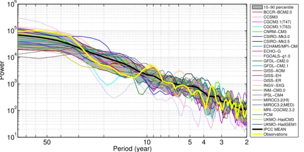
The spatial pattern of the sea surface temperature (SST) field associated with the AMO index is shown in Fig. 1. In the observations there is an overall high positive correlation between the SST and the AMO index for the entire AMO region (shown as square box 5

in the first plot). A region with reduced correlation is seen in the Gulf Stream area and in the Nordic Seas. Most models also show a region of reduced or slightly negative correlation along the North American coast, but for some models this region is shifted slightly north or is distributed over a larger area. Some of the models show polar amplifications of the AMO signal. This is not seen in the observations here due to the 10

lack of data, but has been identified in earlier papers (e.g., Polyakov et al., 2004). Both observations and the majority of models show the strongest correlation between SST and the AMO index in the tropical Atlantic. North of 30◦N the models are more varying.

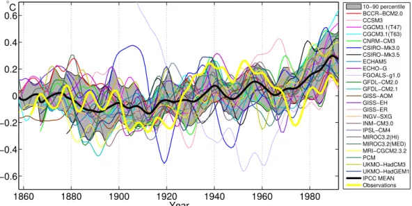
The AMO index for the di_fferent models are shown in Fig. 2a. The mean of the

period 1901–80 has been removed form the models. FGOALS-g1.0 starts from a rel-15

ative warm state, in contrast to the other models and observations. The model has yet to reach a stable equilibrium, and the model has therefore been omitted from the ensemble mean in this figure.

The individual models (thin lines) show highly varying amplitudes, but all models do show a warming in the last two decades when anthropogenic warming becomes 20

influential (IPCC, 2007). Compared to the observations (thick yellow line), the ensem-ble mean (thick black line) shows much less variability. This is to be expected from an average of many independent realizations. For most years the observations are nevertheless reproduced by the model spread, here shown as the 10–90 percentile (gray band). The two main discrepancies between the model spread and the obser-25

(9)

OSD

8, 353–396, 2011

variability

Title Page

Tables Figures

◭ ◮

Back Close

Full Screen / Esc

Discussion

P

a

per

|

Dis

cussion

P

a

per

|

Discussion

P

a

per

|

Discussio

n

P

a

per

|

inadequacy in the modelled response to the external forcing or forcing that is not in-cluded in the simulation, or due to timing of the internal/natural variability in the models compared to observations.

Figure 2b shows the power spectra for the AMO index. The observations have two bands of increased power, one at multidecadal time scales (above∼30 years) and one

5

around 10 years, both being above the level of red noise. Due to varying autocor-relation at lag one for the models and observations, the individual red-noise spectra are not shown. The interannual-decadal power maximum in observations is likely the imprint of the North Atlantic Oscillation on the SST, as this atmospheric mode does show enhanced power at these time scales (Furevik et al., 2003; Hurrell et al., 2003). 10

Most models also show maximum power at multidecadal time scales but with too weak amplitudes compared to the observations. The observed maximum at around 10 years is not captured by the models.

The persistence in the modelled AMO index, defined as the maximum time lag before the autocorrelation function first crosses the significance line at 5% level (Fig. 3), varies 15

from 1 and up to 25 years (Table 2). This indicates the potential for predicting future SSTs based on persistence. For the observations the equivalent persistence time scale is 11 years.

In order to check to what extent the models are able to reproduce the observed warming and cooling patterns, composites of 15 warm years minus 15 cold years are 20

made. Since the models are not able to reproduce the timing of the observed extremes, the simulated warm periods have been selected where the 15 year average temper-ature in each simulation is at its maximum, and the subsequent modelled cold period is then subtracted (Table 2). Due to the anthropogenic warming signal adding to the amplitude of the SST variability towards the end of the time series, warm periods after 25

(10)

OSD

8, 353–396, 2011

variability

Title Page

Tables Figures

◭ ◮

Back Close

Full Screen / Esc

Discussion

P

a

per

|

Dis

cussion

P

a

per

|

Discussion

P

a

per

|

Discussio

n

P

a

per

|

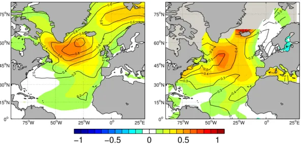
region. Here, the number of models are used as degrees of freedom. The difference between the composites (Fig. 4, left) has the same sign in the whole North Atlantic with largest values in the Subpolar Gyre region to the southeast of Greenland. A warm tongue is also seen extending from the Nordic Seas and into the Barents Sea. The intermodel spread (thin black lines) roughly follows the pattern of the anomaly. The 5

largest model spread is found in the Subpolar Gyre region including the Irminger Sea, with almost the same amplitude as the differences between the warm and cold com-posites. In the tropical Atlantic there is only marginally higher temperatures in the warm compared to the cold periods. In order to see how sensitive this signal is to the chosen warm and cold periods, differences between all warm minus all cold 15 year periods 10

in the models have also been calculated. This analysis gives approximately the same results (not shown).

The observed SST difference between a warm (1941–55) and a cold (1967–81)

15 year period (Fig. 4, right) shows a warm anomaly mainly focused in the center of the Subpolar Gyre and around Iceland. The year to year standard deviation of the 15

observed time series (thin black lines) shows that most of the temperature variance is found in the regions of largest temperature differences. The choice of warm period in the observations could potentially be problematic due to changes in the sampling technique (Thompson et al., 2008). Changing from warm biased engine room intake measurements (US ships) to a temporary majority of uninsulated bucket measurement 20

(UK ships) may have made the cooling trend in the data larger than in reality. To test the robustness of the results, we have shifted the period forward or backward in time. The pattern stays the same but with a slightly reduced amplitude when omitting most of the a_ffected time period (not shown). Comparison with the models show that the regions with largest temperature differences are south of Greenland for both cases, but 25

(11)

OSD

8, 353–396, 2011

variability

Title Page

Tables Figures

◭ ◮

Back Close

Full Screen / Esc

Discussion

P

a

per

|

Dis

cussion

P

a

per

|

Discussion

P

a

per

|

Discussio

n

P

a

per

|

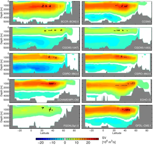
3.2 AMOC

The models show highly varying structures in the mean state of their overturning (Fig. 5). The positions of the maximum overturning are typically found at 600–1500 m depth and between 20◦_{N and 60}◦_{N. In comparison, the estimated depth of the}

max-imum overturning at 25◦_{N is from observations around 1000 m (Bryden et al., 2005).}

5

There are large differences in how the models reproduce the lower overturning cell. Several models show either an absent or a very weak lower overturning cell of Antarc-tic Bottom Water (AABW), while other models show AABW all the way north to 60◦_N.

Hydrographic observations show that the AABW has almost disappeared north of 35◦N (Johnson, 2008). One model, INM-CM3.0, show a deep gyre-driven upper circulation 10

where the subtropical and subpolar gyres are nearly decoupled and where the AABW cell seems to be disconnected from the regions of AABW formation.

The models show an annual mean overturning circulation range from 1.3 to 67.7 Sv, with a long term mean between 7.6 and 39.6 Sv. Based on hydrography,

present-day estimates of the AMOC strength are 14–18 Sv at 24◦N (Ganachaud and Wunch,

15

2000; Lumpkin and Speer, 2003) and 13–19 Sv at 48◦N (Ganachaud, 2003).

Aver-age values from estimates of NADW formation rate are 17.2 Sv (Smethie and Fine, 2001) and 18 Sv (Talley et al., 2003) with an error of ±3–5 Sv. Observations from

hydrographic sections at 26.5◦N measured in the period 2004–2005, show year-long average overturning of 18.7±5.6 Sv (Cunningham et al., 2007). Taking all the

obser-20

vations together, this gives an observed range of 13–24.3 Sv. Many models are outside these estimates (Fig. 6a). GISS-AOM, INM-CM3.0, GISS-ER and GISS-EH show too strong, while FGOALS-g1.0, CGCM3.1(T47 and T63) and IPSL-CM4 show too weak overturning compared to the observations. The remaining 10 of the 18 models have a mean overturning within the observed range, and we will focus on this subset of models 25

in the subsequent analysis.

(12)

OSD

8, 353–396, 2011

variability

Title Page

Tables Figures

◭ ◮

Back Close

Full Screen / Esc

Discussion

P

a

per

|

Dis

cussion

P

a

per

|

Discussion

P

a

per

|

Discussio

n

P

a

per

|

models have maximum energy around the red noise level (not shown due to the vary-ing autocorrelation at lag one defined in Sect. 2), but some show a decrease in power for periods from around 30 years and longer.

For the individual models the persistence in the AMOC variability varies from 1 to 10 years (Table 3), defined as the maximum time lag before the autocorrelation function 5

first crosses the significance line at the 5% level (Fig. 7).

3.3 Surface response to AMOC variability

Figure 8a shows the spatial pattern for the ensemble-mean surface temperature (TS) difference composite for a strong 15 year period minus a weak 15 year period of the AMOC index (see Table 3). The periods are selected where the 15 year average AMOC 10

strength is at a maximum and the subsequent period of low AMOC strength subtracted. An exception has been made if the time series start from or end with the strong or weak AMOC, respectively, since it is unclear whether this is the actual maximum/minimum of the period. For strong AMOC the temperature in the northern North Atlantic and central Nordic Seas is reaching 0.9◦C higher than for weak AMOC. Compared to the 15

magnitude found for warm minus cold phases of AMO in the Subpolar Gyre region (Fig. 4, left), the AMOC composite has a larger temperature difference, and the region of maximum temperature response is slightly displaced northeastward. In the Nordic Seas there is a substantial di_fference between the AMO and AMOC composites. Only for the tropical Atlantic, weak or even negative temperature di_fferences are found for 20

strong minus weak AMOC. The intermodel spread is very large over Iceland and Den-mark Strait and into the Nordic Seas, and the signal to noise ration is low in these areas. The model spread seems to be partly due to the very variable sea ice extent in the different models, where some models have sea ice and others do not in these areas.

25

(13)

OSD

8, 353–396, 2011

variability

Title Page

Tables Figures

◭ ◮

Back Close

Full Screen / Esc

Discussion

P

a

per

|

Dis

cussion

P

a

per

|

Discussion

P

a

per

|

Discussio

n

P

a

per

|

ice extent in the Greenland Sea is mainly unchanged or decreased for strong AMOC and increased sea ice extent for weak AMOC compared to the mean (not shown). In the Barents Sea all models show increased sea ice extent for a weak AMOC, while the results are not conclusive for a strong AMOC. In the Labrador Sea the models show diverging results. The models with less sea ice are the same models that show higher 5

temperatures for strong compared to weak AMOC.

3.4 Covariance between AMOC and AMO in models

The low pass filtered and linearly detrended annual mean time series for the AMOC and AMO indices are shown in Fig. 9. The values and lags for the maximum correlations between the time series are shown in Table 4. Positive lag indicates that AMOC is 10

leading the AMO, e.g., after a strong AMOC the North Atlantic SSTs will tend to be high some years later. All models show the maximum correlation at positive lag. The time lags of variy between 1 and 29 years, and the correlation varies between 0.04 (not significant) and 0.81. Thus the maximum variance that can be explained by the covariance is in the order of 65% or less.

15

Assuming that the North Atlantic becomes warmer when AMOC is stronger than normal, and colder when AMOC is weak, the rate-of-change of AMO should be a better proxy for AMOC than the actual magnitude of the AMO index itself (Fig. 10). With three exceptions (BCCR-BCM2.0, CSIRO-Mk3.5, MIROC3.2(MED)), the analysis does show that AMOC and rate-of-change of AMO is closer to be in phase (Table 4), 20

indicating that there is a linkage between AMOC strength and warming or cooling of the Atlantic surface waters.

4 Discussion

A number of observational studies have shown multidecadal variability in the North Atlantic climate, with a typical time scale of around 50–70 years (e.g., Bjerknes, 25

(14)

OSD

8, 353–396, 2011

variability

Title Page

Tables Figures

◭ ◮

Back Close

Full Screen / Esc

Discussion

P

a

per

|

Dis

cussion

P

a

per

|

Discussion

P

a

per

|

Discussio

n

P

a

per

|

Kravtsov and Spannagle, 2008), and a polar amplification of the climate variations (Furevik, 2001; Polyakov et al., 2004). 20th century extremes are the so-called early warming signal in the 1930s–50s (Delworth and Knutson, 2000) followed by the colder 1960s–80s, and also the very strong North Atlantic and Arctic warming after the 1990s may partly be due to a positive phasing of this mode (e.g., Knight et al., 2005; Zhang 5

et al., 2007; Knight, 2009). Although many of the climate models are able to give rea-sonable amplitudes and to some extent the durations of the climate fluctuations in the North Atlantic region, they are not able to reproduce the timing of the observed warm and cold periods in our analysis. This indicates that the variability is intrinsic to the cli-mate system and not primarily externally forced. This is in agreement with the findings 10

of Kravtsov and Spannagle (2008), Knight (2009) and Ting et al. (2009), where a sub-set of the IPCC AR4 models was analysed. Other possibilities for the discrepancies, such as errors in the observed time series, inadequacy in the modelled response to the external forcing or forcing that is not included in the simulations have been studied thor-oughly in Knight (2009), hence will not be discussed here. Other model simulations, on 15

the other hand, indicate that both solar variability and volcanoes play a role in setting the phase of the variability (Hansen et al., 2005; Otter ˚a et al., 2010). The models are in general able to reproduce the pattern of the recent surface temperature extremes in most of the North Atlantic, but amplitudes seem to be too small in the Iceland Sea and too large in the Norwegian Sea compared to observations. Comparing warm minus 20

cold AMO state, there is no sign of the observed polar amplification in the models. This indicates that the polar amplification is not in phase with the AMO.

For strong AMOC, the multi-model ensemble mean shows anomalously high tem-peratures in the mid and high latitudes (Fig. 8a), and also lower than normal sea ice extent in the Arctic (Fig. 8b). The most plausible mechanism supported by most mod-25

(15)

OSD

8, 353–396, 2011

variability

Title Page

Tables Figures

◭ ◮

Back Close

Full Screen / Esc

Discussion

P

a

per

|

Dis

cussion

P

a

per

|

Discussion

P

a

per

|

Discussio

n

P

a

per

|

move the sea ice edge towards south by advection or local freezing, and more dense water is formed due to cooling and possibly also brine release. This will consequently lead to a strengthening of the overturning circulation (Hawkins and Sutton, 2007). The various mechanisms taking place in the individual models have not been the focus of this study and will not be discussed further.

5

Both the simulated and observed AMO indicate a potential for decadal predictability. While the observations show an inherent AMO persistence of around 11 years, the models have a memory of 1–25 years (Fig. 3). A similar range is found for the modelled AMOC variability, although long persistence of a signal in one parameter does not necessarily imply the same in the other of the two indices of North Atlantic variability. 10

All models are found to have maximum correlation when AMO is lagging AMOC, with lags varying in the range of 1 to 29 years, indicating that AMO variability might be a response to the AMOC variability. When AMOC is found to lead AMO by several decades, an out-of-phase relationship between AMO and AMOC may be expected at shorter lags. This is only found for CSIRO-Mk3.5. For the others such relations are not 15

found due to quasi-periodic time series. In 7 out of 10 models, AMOC is in phase with the rate-of-change of AMO, indicating that through changes in the northward advection of ocean heat, the sea surface temperature starts to respond. The overall results are the same whether we are using the AMO definition of Latif et al. (2004) (50–10◦W, 40–60◦_{N), Sutton and Hodson (2005) (75–7.5}◦_{W, 0–60}◦_{N) or the dipole pattern from}

20

Keenlyside et al. (2008) (60–10◦_{W, 40–60}◦_{N minus 50–0}◦_{W, 40–60}◦_{S), although the}

individual results will change slightly for the individual models.

We should expect that if advection of heat plays a key role in the AMO variability there should be a simple relationship between the strength of the overturning and the frequency of the variability, as long as the volume of the active basins are the same. 25

(16)

OSD

8, 353–396, 2011

variability

Title Page

Tables Figures

◭ ◮

Back Close

Full Screen / Esc

Discussion

P

a

per

|

Dis

cussion

P

a

per

|

Discussion

P

a

per

|

Discussio

n

P

a

per

|

SPG box become

d

d tM=V1ρ1−V2ρ2−QWρW, (1)

d

d t(McpT2)=V1ρ1cpT1−V2ρ2cpT2−QH, (2) d

d tMS2=V1ρ1S1−V2ρ2S2, (3)

whereM is the mass of the water in the mixed layer of the SPG region (here the full 5

water column),V₁and V₂ are the volume transports andρ₁,T₁,S₁ and ρ₂,T₂,S₂ are the densities, temperatures and salinities of water entering or leaving the SPG box, respectively. The net atmospheric freshwater and heat fluxes are given byQW [m3s−1]

and QH [J s−1], defined positive upwards, cp the specific heat capacity, and ρW the

density of the evaporating water. 10

To get the salinity balance in terms of fresh water content, we divide the salinity conservation equation (Eq. 3) on a reference salinity (S₀) and subtract from the mass conservation equation (Eq. 1). Using the Boussinesq approximation, neglecting evap-oration minus precipitation in the mass conservation equation, and assuming conser-vation of volume gives the balance

15

V₁=V₂, (4)

d T₂ d t +

V₂ρ₀ M T2=

V₁ρ₀ M T1−

Q_H

Mc_p, (5)

d S2 d t +

V₂ρ₀ M S2=

V₁ρ₀ M S1+

S₀ρ₀Q_W

M , (6)

whereρ₀is a reference density.

Equation 5 is a simple first order differential equation on the formd T/d t+T/τ=k, 20

(17)

OSD

8, 353–396, 2011

variability

Title Page

Tables Figures

◭ ◮

Back Close

Full Screen / Esc

Discussion

P

a

per

|

Dis

cussion

P

a

per

|

Discussion

P

a

per

|

Discussio

n

P

a

per

|

is therefore omitted). τ is the flushing time scale of the system, i.e. the time it would have taken for the inflowing water to fill the volume of the SPG,k is a measure of the amount of heat entering the system. With constant coe_fficients τ and k the simple solution becomes

T(t)₌(T₀−kτ)e−t/τ+kτ (7)

5

whereT₀is the temperature att=0. Using the size of the region where the temperature is most sensitive to changes in overturning strength (Fig. 8a), i.e. 45–65◦_{N, 50–10}◦_W

givesM=Area_×Depth_×ρ₀≈5.6×1018kg, where the mixing depth is set to 1000 m

due to the depth range of the upper North Atlantic Deep Water (Bryden et al., 2005)

and ρ0 is set to 1000 kg m−3. Based on WOCE estimates (Ganachaud and Wunch,

10

2000) the mean flow into the SPG region through 48◦_{N has been estimated to} _V 1 =

14 Sv which from conservation of mass in the simple model equals the return flow at depth (V2). This gives a flushing time ofτ =13 years which may be interpreted as a

time scale for persistance. Although not directly comparable, this is similar to the 11 years estimated from the autocorrelation of the observed AMO variability (Fig. 3). It 15

is reasonable that the persistence is shorter than the flushing time since the latter is a measure for when all of the water is exchanged, while the former is a measure for when a temperature signal is lost through mixing with surrounding water. Also atmospheric variability will lower the persistence.

There are several studies indicating a relationship between the large scale north-20

south density gradient and the overturning circulation, where a larger depth integrated density gradient is associated with a stronger overturning (Thorpe et al., 2001, and references therein). If more heat is transported into the sinking region, reduced density in the SPG will reduce the north-south density gradient and thus reduce the inflow strength. The result will be gradually colder water and a reversed phase. The time 25

scale of this fluctuating behavior will depend onτ, the flushing time scale, with large flushing time scalesτindicating more long-periodic behavior.

(18)

OSD

8, 353–396, 2011

variability

Title Page

Tables Figures

◭ ◮

Back Close

Full Screen / Esc

Discussion

P

a

per

|

Dis

cussion

P

a

per

|

Discussion

P

a

per

|

Discussio

n

P

a

per

|

strength of the overturning. This will increase the residence time of the water in sub-tropical Atlantic, give a more net evaporation, and lead to a positive salinity anomaly being transported into the sinking region. This will in turn restore the north-south den-sity gradient and speed up the overturning circulation. This mechanism is seen in a freshwater hosing experiment (Otter ˚a et al., 2003). As the relative importance of the 5

temperature and salinity anomalies in determining the density in the convective re-gions varies between the models, the mechanisms and thus the dominant time scales are expected to be highly model dependent (Delworth et al., 1993; Thorpe et al., 2001). It should be noted finally that if there is a direct link between the strength of the AMOC and the AMO, irrespective of which mechanisms are at play, the periodicities of 10

the two time series should be expected to be similar. Based on flushing time scales, the models with the strongest overturning circulation would be expected to be the same as those having the shortest memory if ocean advection is the dominant mechanism. For most models we find a clear link between the AMOC and AMO time scales, but no relation is found between the memory in the system and the strength of the overturning 15

(Fig. 12). This clearly indicates that even if ocean advection (AMOC) plays an important role for the AMO variability, there are other factors such as non-predictable stochastic forcing from the atmosphere or externally forced variability that is masking the signal.

5 Summary and concluding remarks

Simulated variability in the North Atlantic has been investigated and compared with 20

observations. Focus has been on the basin-scale averaged sea surface temperature variability known as the Atlantic Multidecadal Oscillation (AMO), and on the northward upper ocean transports associated with the Atlantic Meridional Overturning Circula-tion (AMOC). For the first time the full suit of IPCC AR4 atmosphere-ocean general circulation models have been used for this purpose. The models show most variabil-25

(19)

OSD

8, 353–396, 2011

variability

Title Page

Tables Figures

◭ ◮

Back Close

Full Screen / Esc

Discussion

P

a

per

|

Dis

cussion

P

a

per

|

Discussion

P

a

per

|

Discussio

n

P

a

per

|

frequencies. The AMOC is found to lead the AMO in all models, and for 7 out of the 10 models showing most realistic AMOC strength, AMOC is close to being in phase with the rate-of-change of AMO suggesting that increased northward heat transport warms the surface ocean.

The spatial structures and amplitude of the simulated temperature anomalies are 5

similar to the observed, but the models fail to capture the timing of the observed ex-tremes, indicating that they are primarily due to internally generated variability and not externally forced.

Most models show a realistic structure of the overturning circulation. This includes both the upper North Atlantic (AMOC) cell and the lower Antarctic overturning cell, 10

and 10 out of 18 models show values within the observationally-based estimate of the range of 13–24.3 Sv for the North Atlantic overturning.

Associated with a stronger AMOC the models shows a positive temperature anomaly and reduced sea ice extent in both the Nordic Seas and in the Labrador Sea compared to a weak AMOC.

15

From a simple conceptual model connecting flushing time scales of a tempera-ture/salinity anomaly to the overturning circulation through the north-south density gra-dient, there is a potential mechanism for decadal predictability of the SSTs if the AMOC state is known. However, from the model results, it is not possible to identify a common mechanism responsible for the variability associated with the AMO, or evidence that ob-20

servations of the surface properties of the ocean (e.g., AMO) automatically can be used as a proxy for the state of the overturning, as suggested by Collins et al. (2006), Smith et al. (2007) and Keenlyside et al. (2008). Hence the road toward future operational decadal predictions of North Atlantic or global climate should involve a full 3-D assimi-lation of the state of the ocean, including both sea level height anomaly from satellites 25

(20)

OSD

8, 353–396, 2011

variability

Title Page

Tables Figures

◭ ◮

Back Close

Full Screen / Esc

Discussion

P

a

per

|

Dis

cussion

P

a

per

|

Discussion

P

a

per

|

Discussio

n

P

a

per

|

Acknowledgements. The project has been supported by the Research Council of Norway through the NorClim project, and is also contributing to the BIAC and DecCen projects. The authors would like to thank Asgeir Sorteberg for help throughout the work, and Nils Gunnar Kvamstø and David Stephenson for useful comments to an earlier draft.

References

5

Baringer, M. O. and Molinari, R.: Atlantic Ocean baroclinic heat flux at 24 to 26◦_{N, Geophys.}

Res. Lett., 26, 353–356, 1999. 356

Bartlett, M. S.: An introduction to stochastic processes. Cambridge University Press, 1966. 359 Bentsen, M., Drange, H., Furevik, T., and Zhou, T.: Simulated variability of the Atlantic merid-ional overturning circulation, Clim. Dynam., 22, 701–720, doi:10.1007/s00382-004-0397-x,

10

2004. 356

Bjerknes, J.: Atlantic air-sea interaction, edited by: Landsberg, H. E. and Van Mieghem, J., Adv. Geophys., Academic press, 1–82, 1964. 355, 365

Bryden, H. L., Longworth, H. R., and Cunningham, S. A.: Slowing of the Atlantic meridional

overturning circulation at 25◦_{N. Nature, 438, 655–657, doi:10.1038/nature04385, 2005. 363,}

15

369

Collins, M., Botzet, M., Carril, A. F., Drange, H., Jouzeau, A., Latif, M., Masina, S., Otter ˚a, O. H., Pohlmann, H., Sorteberg, A., Sutton, R., and Terray, L.: Interannual to decadal climate predictability in the North Atlantic: a multimodel-ensemble study, J. Climate, 19(7), 1195– 1203, 2006. 356, 371

20

Cunningham, S. A., Kanzow, T., Rayner, D., Baringer, M. O., Johns, W. E., Marotzke, J., Long-worth, H. R., Grand, E. M., Hirschi, J. J. M., Beal, L. M., Meinen, C. S., and Bryden, H. L.:

Temporal variability for the Atlantic Meridional Overturning Circulation at 26.5◦_{N, Science,}

317, 935–937, doi:10.1126/science.1141304, 2007. 357, 363

Delworth, T. L. and Knutson, T. R.: imulation of early 20th century global warming, Science,

25

287(5461), 2246–2250, 2000. 366

Delworth, T. L., Manabe, S. and Stouffer, R. J.: Interdecadal variation in the thermohaline

(21)

OSD

8, 353–396, 2011

variability

Title Page

Tables Figures

◭ ◮

Back Close

Full Screen / Esc

Discussion

P

a

per

|

Dis

cussion

P

a

per

|

Discussion

P

a

per

|

Discussio

n

P

a

per

|

Delworth, T. L. and Mann, M. E.: Observed and simulated multidecadal variability in the North-ern hemisphere, Clim. Dynam., 16, 661–676, 2000. 355, 365

Delworth, T. L., Clark, P. U., Holland, M., Johns, W. E., Kuhlbrodt, T., Lynch-Stieglitz, J., Mor-rill, C., Seager, R., Weaver, A. J., and Zhang, R.: The potential for abrupt change in the Atlantic Meridional Overturning Circulation. Abrupt Climate Change, A report by the U.S.,

5

Climate Change Science Program and the Subcommittee on Global Change Research, U.S. Geological Survey, Reston, VA, chap. 4, 117–162, 2008. 355

Deshayes, J. and Frankignoul, C.: Simulated variability of the circulation of the North Atlantic from 1953 to 2003. J. Climate, 21, 4919–4933, doi:11.1175/2008JCLI1882.1, 2008. 356 Dickson, R., Lazier, J., Meincke, J., Rhines, P., and Swift, J.: Long-term coordinated changes

10

in the convective activity of the North Atlantic, Prog. Oceanogr., 38, 241–295, 1996. 356 Dunstone, N. J. and Smith, D. M.: Impact of atmosphere and sub-surface ocean data on

decadal climate prediction, Geophys. Res. Lett., 37, L02709, doi:10.1029/2009GL041609, 2010. 371

Eden, C. and Willebrand, J.: Mechanisms of interannual to decadal variability of the North

15

Atlantic circulation, J. Climate, 14, 2266–2280, 2001. 356

Frankcombe, L. M., Dijkstra, H. A., and von der Heydt, A.: Noise-induced multidecadal vari-ability in the North Atlantic: Excitation of normal modes, J. Phys. Oceanogr., 39, 220–233, doi:10.1175/2008JPO3951.1, 2009. 356

Frankignoul, C., M ¨uller, P., and Zorita, E.: A simple model of the decadal response of the ocean

20

to stochastic wind forcing, J. Phys. Oceanogr., 27, 1533–1546, 1997. 356

Fuglister, F. C.: Atlantic Ocean Atlas of temperature and salinity profiles and data from the international geophysical year of 1957–1958, Woods Hole Oceanogr Inst Atlas Series, Vol. 1, Woods Hole Oceanographic Institution, Woods Hole, Mass, 1960. 356

Furevik, T.: Annual and interannual variability of Atlantic Water temperatures in the Norwegian

25

and Barents Seas: 1980-1996. Deep-Sea Res. Pt. I, 48(2), 383–404, 2001. 355, 366 Furevik, T., Bentsen, M., Drange, H., Kindem, I. K. T., Kvamstø, N. G., and Sorteberg, A.:

Description and evaluation of the Bergen climate model: ARPEGE coupled with MICOM, Clim. Dynam., 21, 27–51, doi:10.1007/s00383-003-0317-5, 2003. 361

Ganachaud, A.: Large-scale mass transports, water mass formation, and diffusivities estimated

30

from World Ocean Circulation Experiment (WOCE) hydrographic data, J. Geophys. Res., 108(C7), 3213, doi:10.1029/2002JC001565, 2003. 363

(22)

OSD

8, 353–396, 2011

variability

Title Page

Tables Figures

◭ ◮

Back Close

Full Screen / Esc

Discussion

P

a

per

|

Dis

cussion

P

a

per

|

Discussion

P

a

per

|

Discussio

n

P

a

per

|

and mixing from hydrographic data, Nature, 408, 453–457, 2000. 359, 363, 369

Gijbels, I., Pope, A., and Wand, M. P.: Understanding exponential smoothing via kernel regres-sion, J. R. Stat. Soc. B, 61(1), 39–50, 1999. 358

Gould, J.: From shallow floats to Argo-The development of neutrally buoyant floats, Deep-Sea Res. Pt. II, 52, 529–543, 2005. 371

5

Hansen, J., Nazarenko, L., Ruedy, R., Sato, M., Willis, J., Del Genio, A., Koch, D., Lacis, A., Lo, K., Menon, S., Navakov, T., Perlwiz, J., Russel, G., Schmidt, G. A., and Tausenev, N.: Earth’s energy imbalance: confirmation and implications, Science, 308, 1431, doi:10.1126/science.1110252, 2005. 355, 366

Hasselmann, K.: Stochastic climate models, Part I, theory, Tellus, 28, 473–483, 1976. 356

10

Hawkins, E. and Sutton, R.: Variability of the Atlantic thermohaline circulation

de-scribed by three-dimensional empirical orthogonal functions. Clim. Dynam., 29, 745–762, doi:10.1007/s00382-007-0263-8, 2007. 367

H ¨akkinen, S.: Variability of the simulated meridional heat transport in the North Atlantic for the period 1951–1993, J. Geophys. Res., 104(C5), 10991–11007, 1999. 356

15

Hurrell, J. W., Kushnir, Y., Ottersen, G., and Visbeck, M.: An overview of the North Atlantic Oscillation, The North Atlantic Oscillation: Climatic significance and environmental impact, edited by: Hurrell, J. W., Kushnir, Y., Ottersen, G., and Visbeck, M., American Geophysical Union, Geoph. Monog. Series, 134, 1–35, 2003. 361

IPCC, 2007: Climate Change 2007: The physical science basis. Contribution of Working Group

20

I to the Fourth Assessment Report of the Intergovernmental Panel on Climate Change, Cam-bridge University Press, CamCam-bridge, United Kingdom and New York, NY, USA. 360

Johnson, G. C.: Quantifying Antarctic Bottom Water and North Atlantic Deep Water volumes, J. Geophys. Res., 113, C05027, doi:10.1029/2007JC004477, 2008. 363

Jungclaus, J. H., Haak, H., Latif, M., and Mikolajewicz, U.: Arctic-North Atlantic interactions and

25

multidecadal variability of the meridional overturning circulation, J. Climate, 18(19), 4013– 4031, 2005. 356

Kaplan, A., Cane, M., Kushnir, Y., Clement, A., Blumenthal, M., and Rajagopalan, B.: Analyses of global sea surface temperature 1856–1991, J. Geophys. Res., 103, 18567–18589, 1998. 359, 386

30

(23)

OSD

8, 353–396, 2011

variability

Title Page

Tables Figures

◭ ◮

Back Close

Full Screen / Esc

Discussion

P

a

per

|

Dis

cussion

P

a

per

|

Discussion

P

a

per

|

Discussio

n

P

a

per

|

Knight, J. R.: The Atlantic Multidecadal Oscillation inferred from the forced

cli-mate response in coupled general circulation models, J. Clicli-mate, 22, 1610–1625, doi:10.1175/2008JCLI2628.1, 2009. 355, 366

Knight, J. R., Allan, R. J., Folland, C. K., Vellinga, M., and Mann, M. E.: A signature of persistent natural thermohaline circulation cycles in observed climate, Geophys. Res. Lett., 32, L20708,

5

doi:10.1029/2006GL026242, 2005. 356, 358, 366

Kravtsov, S. and Spannagle, C.: Multidecadal climate variability in observed and modeled sur-face temperatures, J. Climate, 21, 1104–1121, doi:10.1175/2007JCLI1874.1, 2008. 355, 366

Kushnir, Y.: Interdecadal variations in North Atlantic sea surface temperature and associated

10

atmospheric conditions, J. Climate, 7(1), 141–157, 1994. 355, 365

Latif, M., Roeckner, E., Botzet, M., Esch, M., Haak, H., Hagemann, S., Jungclaus, J. H., Legutke, S., Marsland, S., and Mickolajevicz, U.: Reconstructing, monitoring, and predicting multidecadal-scale changes in the North Atlantic thermohaline circulation with sea surface temperature, J. Climate, 17, 1605–1613, 2004. 355, 367

15

Lumpkin, R. and Speer, K.: Large-scale vertical and horizontal circulation in the North Atlantic Ocean, J. Phys. Oceanogr., 33, 1902–1920, 2003. 363

Marshall, J., Kushnir, Y., Battisti, D., Chang, P., Czaja, A., Dickson, R., Hurrell, J., McCartney, M., Saravanan, R., and Visbeck, M.: North Atlantic climate variability: Phenomena, impacts and mechanisms, Int. J. Climatol., 21, 1863–1898, 2001. 356

20

Medhaug, I., Langehaug, H. R., Eldevik, T., and Furevik, T.: Mechanisms for multidecadal variability in a simulated Atlantic Meridional Overturning Circulation, in prep., 2011. 356, 366 Msadek, R. and Frankignoul, C.: Atlantic multidecadal oceanic variability and its influence on the atmosphere in a climate model, Clim. Dynam., 33, 45–62, doi:10.1007/s00382-008-0452-0, 2009. 356

25

Otter ˚a, O. H., Bentsen, M., Drange, H., and Suo, L.: External forcing as a metronome for Atlantic multidecadal variability, Nat. Geosci., 3, 688–694, doi:10.1038/ngeo955, 2010. 355, 366

Otter ˚a, O. H., Drange,H., Bentsen, M., Kvamstø, N. G., and Jiang, D.: The sensitivity of the present-day Atlantic meridional overturning circulation to freshwater forcing, Geophys. Res.

30

Lett., 30(17), 1898, doi:10.1029/2003GL017578, 2003. 370

(24)

OSD

8, 353–396, 2011

variability

Title Page

Tables Figures

◭ ◮

Back Close

Full Screen / Esc

Discussion

P

a

per

|

Dis

cussion

P

a

per

|

Discussion

P

a

per

|

Discussio

n

P

a

per

|

Pohlmann, H., Jungclaus, J., K ¨ohl, A., Stammer, D., and Marotzke, J.: Initializing decadal

cli-mate prediction with the GECCO oceanic synthesis: Effects on the North Atlantic, J. Climate,

22, 3926–3938, 2009. 356

Polyakov, I. V. and Johnson, M. A.: Arctic decadal and interdecadal variability, Geophys. Res. Lett., 27(24), 4097–4100, 2000. 355

5

Polyakov, I. V., Alekseev, G. V., Timikhov, L. A., Bhatt, U. S., Colony, R. L., Simmons, H. L., Walsh, D., Walsh, J. E., and Zakharov, V. F.: Variability of the Intermediate Atlantic Water of the Arctic Ocean over the last 100 years, J. Climate, 17(23), 4485–4497, 2004. 355, 360, 366

Quenouille, M. H.: Associated Measurements, Butterworths, London, 241 pp., 1952. 359, 381

10

Roemmich, D. and Owens, W. B.: The Argo project: Global ocean observations for understand-ing and prediction of climate variability, Oceanogr., 13, 45–50, 2000. 371

Roemmich, D. and Wunsch, C.: Two transatlantic sections: meridional circulation and heat flux in the subtropical North Atlantic Ocean, Deep-Sea Res., 32, 619–664, 1985. 356

Schlesinger, M. E. and Ramankutty, N.: An oscillation in the global climate system of period

15

65-70 years, Nature, 367, 723–726, 1994. 355, 365

Schott, F. A., McCreary Jr, J. P., and Johnson, G. C.: Shallow overturning circulation of the tropical-subtropical oceans, Earth Climate: The Ocean-Atmosphere Interaction, edited by: Wang, C., Xie, S., and Carton, J. A., American Geophysical Union, Geoph. Monog. Series, 147, 261–304, 2004. 358

20

Smethie, W. M. and Fine, R. A.: Rates of North Atlantic deep water formation calculated from chlorofluorocarbon inventories, Deep-Sea Res. Pt. I, 48, 189–215, 2001. 363

Smith, D. M., Cusack, S., Colman, A. W., Folland, C. K., Harris, G. R., and Murphy, J. M.: Improved surface temperature prediction for the coming decade from a global climate model, Science, 317, 796–799, doi:10.1126/science.1139540, 2007. 356, 371

25

Sutton, R. T. and Hodson, D. L. R.:Atlantic Ocean forcing of North American and European summer climate, Science, 309(5731), 115–118, doi:10.1126/science.110949, 2005. 358, 367

Talley, L. D., Reid, J. L., and Robbins, P. E.: Data-based meridional overturning streamfunctions for the global ocean, J. Climate, 16, 3213–3226, 2003. 359, 363

30

Thompson, D. J.: Spectrum estimation and harmonic analysis, P IEEE, 70(9), 1055–1096, 1982. 359

(25)

OSD

8, 353–396, 2011

variability

Title Page

Tables Figures

◭ ◮

Back Close

Full Screen / Esc

Discussion

P

a

per

|

Dis

cussion

P

a

per

|

Discussion

P

a

per

|

Discussio

n

P

a

per

|

mid-twentieth century in observed global-mean surface temperature, Nature, 453, 646–649, doi:10.1038/nature06982, 2008. 362

Thorpe, R. B., Gregory, J. M., Johns, T. C., Wood, R. A., and Mitchell, J. F. B.: Mechanisms determining the Atlantic thermohaline circulation response to greenhouse gas forcing in a non-flux-adjusted coupled climate model, J. Climate, 14, 3102–3116, 2001. 369, 370

5

Ting, M., Kushnir, Y., Seager, R., and Li, C.: Forced and internal twentieth-century SST trends in the North Atlantic, J. Climate, 22, 1469–1481, doi:10.1175/2008JCLI2561.1, 2009. 355, 366

Trenberth, K. E. and Caron, J. M.: Estimates of meridional atmosphere and ocean heat trans-ports, J. Climate, 14, 3433–3443, 2001. 354

10

Vellinga, M. and Wu, P.: Low-latitude freshwater influence on centennial variability of the At-lantic thermohaline circulation, J. Climate, 17, 4498–4511, doi:10.1175/3219.1, 2004. 356 Woodgate, R. A., Aagaard, K., and Weingartner, T. J.: Monthly temperature, salinity, and

transport variability of the Bering Strait through flow, Geophys. Res. Lett., 32, L04601, doi:10.1029/2004GL021880, 2005. 359

15

Wunsch, C.: What is the thermohaline circulation? Science, 298, 1180–1181, 2002. 355 Zhang, R., Delworth, T. L., and Held, I. M.: Can the Atlantic Ocean drive the observed

(26)

OSD

8, 353–396, 2011

variability

Title Page

Tables Figures

◭ ◮

Back Close

Full Screen / Esc

Discussion

P

a

per

|

Dis

cussion

P

a

per

|

Discussion

P

a

per

|

Discussio

n

P

a

per

|

Table 1.List of models that participate in this study.

Modeling groups IPCC ID Horizontal Natural

Atm. res. forcing Bjerknes Centre for Climate Research, University of Bergen, Norway BCCR-BCM2.0 T63 No National Center for Atmospheric Research, USA CCSM3 T85 Yes Canadian Centre for Climate Modeling & Analysis, Canada CGCM3.1(T47) T47 No CGCM3.1(T63) T63 No M ét éo-France/Centre National de Recherches M ét éorologique, France CNRM-CM3 T63 No CSIRO Atmospheric Research, Australia CSIRO-Mk3.0 T63 No

CSIRO-Mk3.5 T63 No

Max Planck Institute for Meteorology, Germany ECHAM5/MPI-OM T63 No Meteorological Institute of the University of Bonn, ECHO-G T30 Yes

Meteorological Research Institute of KMA, and Model and Data group, Germany/Korea

LASG/Institute of Atmospheric Physics, China FGOALS-g1.0 T42 No NOAA/Geophysical Fluid Dynamics Laboratory, USA GFDL-CM2.0 2.0◦

×2.5◦ _Yes

GFDL-CM2.1 2.0◦

×2.5◦ _Yes

NASA/Goddard Institute for Space Studies, USA GISS-AOM 3◦

×4◦ _No

GISS-EH 4◦

×5◦ _Yes

GISS-ER 4◦

×5◦ _Yes

National Institute of Geophysics and Volcanology, Italy INGV-SXG T106 No Institute for Numerical Mathematics, Russia INM-CM3.0 4◦

×5◦ _Yes

Institute Pierre Simon Laplace, France IPSL-CM4 2.5◦

×3.8◦ _No

Center for Climate System Research, National Institute for MIROC3.2(HI) T106 Yes Environmental Studies, and Frontier Research Center MIROC3.2(MED) T42 Yes for Global Change, Japan

Meteorological Research Institute, Japan MRI-CGCM2.3.2 T42 Yes National Center for Atmospheric Research, USA PCM T42 Yes Hadley Centre for Climate Prediction and Research/Met Office, UK UKMO-HadCM3 2.8◦

×3.8◦ _No

(27)

OSD

8, 353–396, 2011

variability

Title Page

Tables Figures

◭ ◮

Back Close

Full Screen / Esc

Discussion

P

a

per

|

Dis

cussion

P

a

per

|

Discussion

P

a

per

|

Discussio

n

P

a

per

|

Table 2. Warm and subsequent cold 15 year periods (center years) used to make AMO

com-posites. The persistence (τgiven in years) of the AMO time series is taken from the

autocorre-lation function of the annual time series.

Model Warm Cold τ

BCCR-BCM2.0 1879 1918 3

CCSM3 1962 1980 10

CGCM3.1(T47) 1864 1879 13

CGCM3.1(T63) 1923 1943 13

CNRM-CM3 1943 1958 4

CSIRO-Mk3.0 1904 1919 6

CSIRO-Mk3.5 1921 1937 1

ECHAM5/MPI-OM 1946 1966 4

ECHO-G 1945 1975 10

FGOALS-g1.0 – – 25

GFDL-CM2.0 1960 1979 5

GFDL-CM2.1 1936 1950 5

GISS-AOM 1958 1968 2

GISS-EH 1878 1888 3

GISS-ER 1956 1977 3

INGV-SXG 1924 1932 2

INM-CM3.0 1957 1968 1

IPSL-CM4 1925 1940 4

MIROC3.2(HI) 1962 1970 1

MIROC3.2(MED) 1876 1893 4

MRI-CGCM2.3.2 1956 1969 5

PCM 1940 1962 3

UKMO-HadCM3 1878 1897 3

UKMO-HadGEM1 1940 1969 3

(28)

OSD

8, 353–396, 2011

variability

Title Page

Tables Figures

◭ ◮

Back Close

Full Screen / Esc

Discussion

P

a

per

|

Dis

cussion

P

a

per

|

Discussion

P

a

per

|

Discussio

n

P

a

per

|

Table 3. Strong and subsequent weak 15 year periods (center years) used to make AMOC

composites. The persistence (τ given in years) of the AMOC time series is taken from the

autocorrelation function of the annual time series.

Model Strong Weak τ

BCCR-BCM2.0 1933 1949 10

CCSM3 1891 1920 8

CSIRO-Mk3.0 1905 1915 4

CSIRO-Mk3.5 1891 1938 5

ECHAM5/MPI-OM 1905 1923 7

ECHO-G 1881 1902 4

GFDL-CM2.1 1903 1927 5

MIROC3.2(HI) 1933 1948 2

MIROC3.2(MED) 1921 1945 4