Case study of stratospheric gravity waves of convective origin over Arctic Scandinavia – VHF radar observations and numerical modelling

(1)

Ann. Geophys., 31, 239–250, 2013 www.ann-geophys.net/31/239/2013/ doi:10.5194/angeo-31-239-2013

Annales

Geophysicae

Open Access

Geoscientiic

Case study of stratospheric gravity waves of convective origin over

Arctic Scandinavia – VHF radar observations and numerical

modelling

A. R´echou1, J. Arnault2, P. Dalin2, and S. Kirkwood2

1_{Laboratoire de l’Atmosphère et des Cyclones, UMR8105, La Réunion University, 15 avenue René Cassin, BP 7151, 97715}

St. Denis Messag Cedex 9, Ile de La R´eunion, France

2_{Swedish Institute of Space Physics, P.O. Box 812, 981 28 Kiruna, Sweden}

Correspondence to:A. R´echou (arechou@univ-reunion.fr)

Received: 30 October 2012 – Revised: 7 December 2012 – Accepted: 22 January 2013 – Published: 15 February 2013

Abstract.Orography is a well-known source of gravity and inertia-gravity waves in the atmosphere. Other sources, such as convection, are also known to be potentially important but the large amplitude of orographic waves over Scandi-navia has generally precluded the possibility to study such other sources experimentally in this region. In order to bet-ter understand the origin of stratospheric gravity waves ob-served by the VHF radar ESRAD (Esrange MST radar) over Kiruna, in Arctic Sweden (67.88◦N, 21.10◦E), observations have been compared to simulations made using the Weather Research and Forecasting model (WRF) with and without the effects of orography and clouds. This case study con-cerns gravity waves observed from 00:00 UTC on 18 Febru-ary to 12:00 UTC on 20 FebruFebru-ary 2007. We focus on the wave signatures in the static stability field and vertical wind deduced from the simulations and from the observations as these are the parameters which are provided by the obser-vations with the best height coverage. As is common at this site, orographic gravity waves were produced over the Scan-dinavian mountains and observed by the radar. However, at the same time, southward propagation of fronts in the Bar-ents Sea created short-period waves which propagated into the stratosphere and were transported, embedded in the cy-clonic winds, over the radar site.

Keywords. Meteorology and atmospheric dynamics (Con-vective processes; Polar meteorology; waves and tides)

1 Introduction

Atmospheric gravity or inertia-gravity waves are character-ized by fluctuations of vertical velocity, horizontal winds, density and temperature, in a stably stratified environment (e.g. Holton, 1992). When the restoring mechanism is buoy-ancy only, they are called pure internal gravity waves or sim-ply gravity waves, while inertia-gravity waves result from a combination of stratification and Coriolis effects. Inertia-gravity waves are characterized by horizontal scales greater than a few hundred kilometers and periods greater than a few hours, which is the reason why they are also affected by the Coriolis force. Gravity and inertia-gravity waves transport energy and momentum as they propagate either vertically or horizontally. This causes a transfer of energy and momentum from the source of the waves to their sink, where they dissi-pate (Fritts and Alexander, 2003). For these reasons gravity and inertia-gravity waves play a substantial part in determin-ing the circulation of the atmosphere and oceans, which ne-cessitates a better understanding of how these waves gener-ate, evolve and then dissipate (for a review, see Fritts and Alexander, 2003).

The sources of gravity and inertia-gravity waves are nu-merous. They can, for example, be created by orography (e.g. McFarlane, 1987), convection (e.g. Larsen et al., 1982), strong diabatic heating (e.g. Hooke, 1986), jet instability (e.g. Uccellini and Koch, 1987) or wind shear (e.g. Fritts, 1982). In this study we focus primarily on convective and orographic sources.

(2)

(Gossard and Hooke, 1975). These orographically induced gravity waves have also been inferred as a secondary source for inertia-gravity waves in the winter extratropical strato-sphere in numerous observational studies (e.g. Sato, 1994; Worthington, 1999; Serafimovich et al., 2006), and in the fall and spring lower-stratosphere by Eckermann and Preusse (1999).

The convective effect can also be responsible for gravity and inertia-gravity wave generation. Waves created by con-vection are as numerous (i.e. with many different scales) as the generation mechanisms (different convective structures). Convectively-induced waves can for example be triggered by the bulk release of latent heat (Piani et al., 2000), the obsta-cle effect produced by the convective column on the stratified shear flow above (Clark et al., 1986; Mason and Sykes, 1982; Pfister et al., 1993), or the mechanical pump effect due to ver-tical oscillations of updrafts and downdrafts behaving as an oscillating rigid body (Fovell et al., 1992; Alexander et al., 1995; Alexander and Barnett, 2007). All three mechanisms can be coupled, depending strongly upon the local shear and the vertical profile and time dependence of the latent heating (Fritts and Alexander, 2003).

It has also been shown that surface fronts are important sources of gravity waves (Fritts and Nastrom, 1992). Eck-ermann and Vincent (1993) presented case studies of such waves using stratosphere–troposphere (ST) radar observa-tions during the passage of cold fronts over southern Aus-tralia. Snyder et al. (1993) and Griffiths and Reeder (1996) showed, in idealized studies of frontogenesis, that fronts can be significant sources of gravity waves. According to these authors the wave emission becomes more pronounced as the frontal scale contracts, or when the frontogenesis occurs quickly.

Since gravity and inertia-gravity waves are generally not resolved by the synoptic observational network, in situ ob-servations (e.g. aircraft, Brown, 1983; Cui et al., 2012, rockets, Rapp et al., 2004, balloon-borne soundings, Shutts and Broad, 1993) and remote sounding (e.g. Mesosphere-Stratosphere-Troposphere MST radar) provide valuable in-formation for studying their characteristics. Gravity and inertia-gravity waves have been studied at many radar sites around the world, for example, by Sato et al. (1997) and Thomas et al. (1999). Radar or in situ measurements are lo-calized in space and time, so these measurements alone are generally not sufficient to understand the physics of the ob-served waves (e.g. R¨ottger, 2000). High resolution numerical modelling can be a good complement to better characterize the physical processes associated with such waves. Indeed, MST radar measurements, in particular, provide data at an appropriate temporal and vertical resolution to compare with numerical modelling (e.g. Serafimovich et al., 2006; Sato and Yoshiki, 2008; Kirkwood et al., 2010; Valkonen et al., 2010). In almost all earlier studies using radar, wind-perturbations have been used to study gravity waves. However, generally very powerful radars such as the MU

radar in Japan (Sato, 1994) or the Indian MST radar (Dutta et al., 1999) are needed to make sufficiently accurate wind measurements in the stratosphere. VHF radar, in addition to measuring winds, can also be used to measure buoyancy frequency (static stability, e.g. Hooper et al., 2004) and its time/height variations in the lower stratosphere, providing an alternative wave diagnostic to measurements of wind-perturbations. Buoyancy frequency is directly derived from the echo-power measured by a VHF radar and this can be readily measured with high accuracy even by relatively low-power VHF wind profiler radars (see e.g. Arnault and Kirkwood, 2012).

Since buoyancy frequency can be related to gravity wave characteristics according to several idealized and observa-tional case studies (e.g. Humi, 2004, 2010; Shutts et al., 1988, 1994), we will present in this paper a case study of gravity waves observed as fluctuations in buoyancy fre-quency in the lower stratosphere, using the VHF wind pro-filer radar ESRAD located at Esrange (67.9◦N, 21.1◦E) in Sweden. In this case, we find gravity waves with long vertical wavelengths so that it is possible to confirm the wave origin of the buoyancy frequency fluctuations using low-vertical-resolution measurements of vertical wind.

The observations will be complemented with numerical experiments using the WRF (Weather Research and Fore-casting) model in different configurations (with and without orography, with and without clouds). We use spectral anal-ysis to characterize the waves in both ESRAD and WRF data. A comparison with the different configurations used in the WRF modelling allows us to investigate the sources of the different waves observed by ESRAD. But first, we will present the synoptic conditions associated with our study in-terval.

2 Synoptic analysis

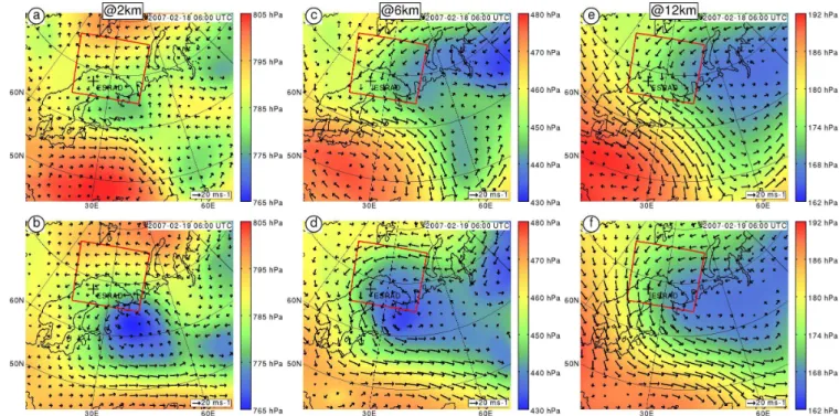
Figure 1 presents the synoptic situation at 06:00 UTC on 18 February 2007 and at 06:00 UTC on 19 February 2007, computed from ECMWF (European Centre for Medium-Range Weather Forecasts) analyses at altitudes 2 km (lower part of the troposphere), 6 km (middle part of the tropo-sphere) and 12 km (lower part of stratotropo-sphere), for an area covering northern Scandinavia and the surrounding ocean.

(3)

A. R´echou et al.: Case study of stratospheric gravity waves of convective origin over Arctic Scandinavia 241

Fig. 1. (a),(b)Horizontal cross sections at 2 km altitude of pressure (colour) in hPa and horizontal winds (arrows) in m s−1at 06:00 UTC on 18 February 2007 and at 06:00 UTC on 19 February 2007, computed with ECMWF analyses. The pressure scale is given by the coloured bar to the right, and the wind scale by the arrow at the bottom right corner of each panel. The red box gives the location of the domain used in the WRF simulation. The black cross gives the location of ESRAD radar.(c),(d)as in(a),(b), except at 6 km altitude.(e),(f)as(a)–(d), except at 12 km altitude.

i.e. in the lower stratosphere, where the low-pressure system in the northeast and east of Scandinavia (polar vortex) is as-sociated with strong cyclonic winds at the ESRAD location, and a high pressure system in the southwest of Scandinavia is associated with anti-cyclonic winds also present in the lower levels (2 and 6 km, Fig. 1a, c). The transition between the two cyclonic and anticyclonic systems occurs in the middle of Scandinavia, where intense northwesterly winds can be observed at 2, 6 and 12 km (Fig. 1a, c, e).

On the 19th, at 2 km, the low-pressure system in the east is more intense with a decrease of about 5 hPa (compare Fig. 1a, b). The polar high in the north has moved further south at this height although it has not reached the conti-nent yet. It is associated to more intense easterly winds in the northern part of Scandinavia. At 6 km and at 12 km, the north of Scandinavia is mainly affected by the low-pressure system from the east (Fig. 1d and f).

3 Radar observations

3.1 Description of ESRAD radar

ESRAD is a 52 MHz atmospheric radar, located at Esrange near Kiruna, Sweden (67.88◦N, 21.10◦E), above the polar circle. At the time of the case study presented here, the sys-tem comprised a transmitter with 72 KW peak power, 6

in-dependent receivers, and a rectangular 16×18 array of 5-element yagi antennas, with 4.04 m spacing of the yagis (0.7 times the radar wavelength). The whole array was used for transmission, but it was divided for reception into 6 sub-arrays, each of 8×6 yagis and each connected to a separate receiver. The measurements used here were made using two interlaced measurement modes, the first using a 1 µs trans-mitted pulse and 1 µs sampling, providing nominal 150 m height resolution (in practice about 200 m taking into account receiver filter effects), and the second using 8-bit comple-mentary codes with 4 µs baud, providing 600 m vertical res-olution. Horizontal winds are derived using time delays be-tween echoes arriving at different sub-arrays, while vertical winds and echo power are derived by combining the mea-surements from all 6 receivers. A detailed description for the ESRAD radar is given by Chilson et al. (1999), updated by Kirkwood et al. (2007).

(4)

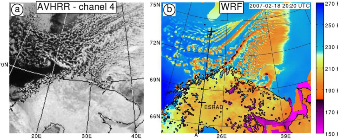
Fig. 2. (a)Advanced Very High Resolution Radiometer (AVHRR) image taken by the polar orbiting NOAA-17 satellite in the thermal infra-red (10.3–11.3 µm) channel 4 at 20:14 UTC on 8 February 2007 (from http://www.sat.dundee.ac.uk).(b)OLR (K) retrieved from the WRF simulation with clouds and orography at 20:20 UTC on 18 February 2007. The brightness temperature scale is given by the coloured bar to the right. The straight black line (A–B) gives the location of the vertical cross sections in Fig. 6. The position of the ESRAD radar is located by a black cross.

in principle determine the radar echo power returned to the receivers (e.g. Gage, 1990). For the lower-stratosphere (and upper-troposphere at high latitudes) humidity is very low, and for measurements by vertically pointing radars operat-ing at around 50 MHz, density and temperature gradient have been found to dominate the atmospheric contribution to the echo power. As a result, echo power can be easily scaled to provide an estimate of static stabilityN:

R=(F zexp(z/H )Pr1/2)1/2, (1)

whereR₌N at heights where humidity is negligible,F is a proportionality constant,z is height,H is the atmospheric scale height, exp(−z/H ) is the height variation of atmo-spheric density,Pris radar echo power (e.g. Hooper et al.,

2004). The constantF can be found either by careful cali-bration of the radar, or more easily, by comparison with ra-diosonde measurements (Kirkwood et al., 2010, 2011). In this case, 5 radiosondes released from Esrange on the 21 and 22 February have been used to determine the value of F (F=0.21±0.01). Values forPrin the lowermost

strato-sphere for this particular (150 m resolution) radar experiment were in the range 10−16to 10−14W.

The temperature fluctuations associated with gravity or/and inertia-gravity waves propagating in the lower strato-sphere lead to corresponding fluctuations in the static stabil-ity (for example, see Arnault and Kirkwood, 2012). Particu-larly in the lower stratosphere, where the radar echo strength is weak, the static stability can be derived from the radar mea-surements with much higher accuracy than the wind fluctua-tions associated with the waves. So we will focus primarily on fluctuations in N in the following analysis of ESRAD-observed lower-stratospheric gravity/inertia-gravity waves. For this study, 20-min averages of the echo power using

the measurements with 150-m vertical resolution, have been used to deriveN.

Although ESRAD was able to measure horizontal winds on this occasion up to heights of about 12–13 km, using the operating mode with low vertical resolution (600 m), the ac-curacy of the wind estimates was not sufficient to determine the wind fluctuations associated with the waves. Indeed, the full correlation analysis (fca) method used to derive horizon-tal winds from the radar data needs relatively strong Signal to Noise Ratio (SNR) to work properly. On the other hand, vertical winds derived from the Doppler frequency need less SNR to be accurate enough, i.e. resolve the wave fluctua-tions considered in this case. Since both the convective-origin wave and the orographic wave have vertical wavelengths which are rather more than 600 m, we can use these verti-cal wind measurements to compare with the vertiverti-cal wind component in the different WRF modelling experiments.

3.2 Buoyancy frequency (N_{) and vertical velocity (}W₎

profile

(5)

687

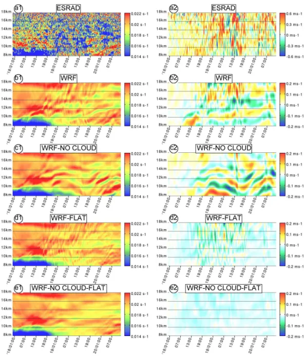
Fig. 3. (a)Time–height diagram of (1) buoyancy frequency (colours) in s−1,and (2) vertical velocity from ESRAD observations. The hori-zontal axis gives the time in days from 00:00 UTC on 18 February 2007 to 12:00 UTC on 20 February 2007, and the vertical axis gives the height in km. The buoyancy frequency and vertical velocity scales are given by the coloured bar on the right of each panel.(b), As in(a), except from the WRF model experiment with clouds and orography.(c), As in(a), except from the WRF model experiment without clouds but with orography.(d), As in(a), except from the WRF model experiment with clouds but without orography.(e), As in(a), except from the WRF model experiment without clouds and without orography.

from 8 km to 12 km with the height of the wavefronts in-creasing over time. Above 12 km height on the 20th, there are descending wavefronts corresponding to apparent peri-ods of several hours, and with vertical wavelengths about 1– 2 km. We can see the same patterns of fluctuations in vertical wind as are seen for buoyancy frequency, with short-period variations (vertical streaks) from about 18:00 UTC on the 18th to 18:00 UTC on the 19th, and slowly changing

quasi-horizontal bands of upward or downward vertical winds later, thus supporting the use of using buoyancy frequency to diag-nose the gravity wave activity in the lower stratosphere.

(6)

it is clear that the tropopause height was around 9 km on 18 February, but dropped below 8 km on 19 and 20 February.

3.3 Spectrum analysis

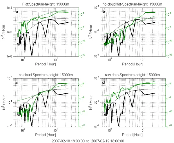
To identify the periodicities observed in the gravity wave packets, we apply spectral analysis to the time series of buoy-ancy frequency as estimated from the ESRAD data (and as calculated with the WRF model, which will be described later). To make it clear which gravity waves periods domi-nate, the multiple-taper method (MTM) has been used to es-timate the power spectral density (PSD) of the variations in the buoyancy frequency (Percival and Walden, 1993). This method uses linear or non-linear combinations of modified periodograms in order to minimize spectral leakage outside of the analyzed spectral band. The shortest period resolved is 40 min, as the ESRAD data were averaged for 20 min. As will become clear in Sect. 4, we are able to identify convective-source waves in the observations on 19 February. In order to study the convective waves in more detail, the radar spectrum was estimated for 15 000 m height for the in-terval 18:00 UTC on 18 February to 18:00 UTC on 19 Febru-ary and is plotted as the black lines in Fig. 4. Also, the fig-ure presents the red noise level and its 95 % confidence level (thin curve in Fig. 4), which has been found in the PSD ac-cording to Mann and Lees (1996). Spectral peaks which are close to and above the 95 % confidence level should be re-garded as significant harmonic oscillations in a given time series.

Note that the “period” axis for the spectra represents ap-parent periods, which may differ from the intrinsic periods depending on the wave propagation direction and the back-ground wind. We use the radar spectrum primarily to com-pare between the observations and different simulation re-sults, as will be discussed in detail in Sect. 4.

4 Numerical simulation

4.1 Setting of the model experiments

The situation is modelled using the Weather Research and Forecasting model (WRF, Skamarock and Klemp, 2008). Four different WRF simulations are used, with and without clouds (resp. WRF-CLOUD and WRF-NO CLOUD), with and without orography (resp. WRF and WRF-FLAT). All use one polar stereographic domain at a horizontal resolu-tion of 6 km (red rectangle in Fig. 1), with 100 vertical lev-els up to 20 hPa (approximately 24 km). The vertical spacing is stretched from 60 m at the lowest to 450 m at the highest level. Rayleigh damping in the uppermost 5 km was intro-duced in order to avoid spurious wave reflection from the model lid (following Durran and Klemp, 1983). The four nu-merical experiments start at 00:00 UTC, 16 February 2007, two days before the period of interest, and are run for five days. They are coupled with ECMWF operational analyses

at the initial time and every 6 h at the boundaries. The model equations are integrated at a time step of 24 s. The model out-puts containing the usual dynamic and thermodynamic vari-ables are then saved every twenty minutes, in order to analyse the short-period waves induced by convection.

For the simulations with clouds, convection is explicit and microphysics is parameterized with the 3-class liquid and ice hydrometeors scheme of Hong et al. (2004). For the simu-lations without clouds no scheme of microphysics is used and the scheme for parameterizing surface fluxes is switched off. Radiative processes are represented with the long- and short-wave radiation schemes of Mlawer et al. (1997) and Dudhia (1989), respectively. The turbulent transport of heat, moisture, and momentum is parameterized in the whole at-mospheric column with the scheme of Hong et al. (2006).

4.2 Comparison with radar observations

The time–height diagrams ofN andW from the radar ob-servations and from the model simulations, at the location of ESRAD, are shown in Fig. 3, covering the 3-day period from the 00:00 UTC on the 18th to 12:00 UTC on the 20th, and from 8 km to 18 km height, i.e. the lower stratosphere. Results in Figs. 3b1 and 3b2 (“WRF”) take into account both orography and cloud microphysical processes, Figs. 3c1 and 3c2 (“WRF-NO CLOUD”), orography without clouds, Figs. 3d1 and 3d2, (“WRF-FLAT”) no orography but with clouds, and Figs. 3e1 and 3e2 (“WRF-NO CLOUD FLAT”), no orography and without clouds.

Comparing the different panels of Fig. 3, provides a first step towards understanding the different origins of the waves observed by ESRAD. Overall, the variations ofN and W seen by ESRAD are well correlated with similar features in the WRF simulations with all forcings present, even if the amplitude seen by the radar is slightly larger (the lowest val-ues ofN are lower in Fig. 3a1 compared to Fig. 3b1, and a different scale has been used for the ESRADWobservations in Fig. 3a2 to accommodate the larger range ofWcompared to the model). It is also clear comparing Fig. 3b with Fig. 3c, d and e, that some groups of features disappear when clouds or orography are removed.

The first feature to note are the short-period waves, most clearly visible from the end of the 18th (18:00 UTC) to the end of the 19th, which are seen only in the simulations in-cluding clouds (Fig. 3b, d). They are completely absent in the simulations without clouds (Fig. 3c, e). The short-period variations can also be discerned in the ESRAD data (Fig. 3a), although, inN, not as clearly as in the model.

(7)

Fig. 4.Spectrum of time series ofNat 15 000 m height, from 18:00 UTC on 18 February 2007 to 18:00 UTC on 19 February 2007. The black line in all panels shows the spectrum obtained from ESRAD, the green lines show the results from the WRF model experiments. The 95 % confidence level (thin green and black curves).(a)simulation with clouds but without orography;(b)simulation without clouds and without orography;(c)simulation without clouds but with orography; and(d)simulation with clouds and with orography.

The spectral analysis during this time (Fig. 4, taken at 15 km altitude between 18 February, 18:00 UTC, and 19 February, 18:00 UTC) also shows that, in the simulations without clouds, the energy for periods below 6 h is much less than in the other simulations.

In the high frequency range (less than one hour) essen-tially nothing occurs in the simulations without clouds. Peaks at 50 min and slightly more than 1 h and 3 h are observed in the spectrum of the ESRAD data and high power is found at these periods in the simulations taking into account the clouds (Fig. 4a, d), but much less than that without the clouds (Fig. 4b, c), the latter not reaching 95 % significance. This suggests that the short-period gravity waves observed by the radar were induced by convection associated with clouds. We will return to the origin of these waves in Sect. 4.3. We can also note that the peaks at 1.5 (significance at 90 %) and 3 h (significance at 95 %) apparent periods seen by ESRAD are best reproduced by the model simulation including both clouds and orographic waves, so they are a result of the inter-action between the two processes. We emphasise that this is mainly an interaction between the waves generated by

con-vection and orographic waves, not between the convective waves and the orography itself, as shown later.

A second group of waves are seen in the simulations in-cluding orography (Fig. 3b, c) but are largely absent in the simulations without orography (Fig. 3d, e). These have about 2 km vertical wavelength with wavefronts sometimes sloping upwards (late on the 18, late 19 to early 20 February), some-times flat (early 19 February), somesome-times downward (morn-ing of 19 February). The correspond(morn-ing features can be seen in the observations (Fig. 3a) starting late on 19 February. They can be discerned earlier on 19 February but they are not so clear because of the shorter period waves which are also present. These are clearly caused by the orography. As quasi-stationary waves, the slope of the wavefronts over time will be very sensitive to the background wind conditions. Oro-graphic waves (7 h period, significant at 95 % in Fig. 4) are well known to occur at this location and they will not be stud-ied in detail in the present case study, except as they interact with the convective waves.

(8)

Fig. 5. (a)–(b)Latitude–longitude cross sections at 12 km altitude of buoyancy frequency (colour) in s−1and horizontal winds (arrows) in m s−1at 06:00 and 18:00 UTC, 19 February 2007, computed from the WRF experiments. The buoyancy frequency scale is given in Fig. 3, and the wind scale by the arrow at the bottom right corner of each panel. The straight black line (A–B) gives the location of the vertical cross sections in Fig. 6. The distance between wind arrows is 80 km. ESRAD radar location is indicated by a black cross along this line. (a1)–(b1)Simulation with clouds and orography;(a2)–(b2)simulation without clouds but with orography;(a3)–(b3)simulation with clouds but without orography.

slowly descending wavefronts with vertical wavelengths of around 1 km. Similar long-period waves are present through-out the interval, in all the simulations, even withthrough-out clouds or orography (Fig. 3b–e), and can also be seen in the observa-tions on 18 February. They are more distinct in the simula-tions including all forcings and quite indistinct in the sim-ulation with neither clouds nor orography. These may be inertia-gravity waves generated by the tropospheric jet. For example, Hoffman et al. (2006) have shown an example of inertia-gravity waves generated by a jet-streak which were locally enhanced by mountain waves above the Scandinavian Ridge. Further study of these waves is beyond the scope of the present case study, which concentrates on the convective waves.

Since we have no direct measurements of accurate hori-zontal wind and its fluctuations, for this case study, in the stratosphere above Esrange, we cannot apply the usual kind of analysis (Gerrard et al., 2004, 2011; Dalin et al., 2004) to estimate a complete set of gravity wave parameters. It is pos-sible to retrieve the information on the horizontal wind, and

the wave fluctuations in the horizontal wind, from the model, but this topic is beyond the scope of the present paper.

4.3 Convective source investigation

In order to investigate the sources of the short-period waves in more detail, the distribution of waves over the whole simulation domain is examined. Figure 5 shows latitude– longitude cross sections ofN obtained by the different WRF simulations, at 12 km altitude, at 06:00 UTC and 18:00 UTC on 19 February. In Fig. 5, most clearly on 19 February (Fig. 5a1, 5a3), waves with short horizontal wavelength can be seen in the simulations with clouds, over the ocean to the north of Scandinavia (north of 72◦_{latitude). Figure 6 shows}

(9)

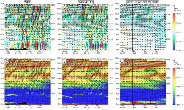
Fig. 6. (a)–(f)Vertical south–north cross sections at the location indicated by the line (A–B) in Figs. 2b and 5, for the vertical wind component (a,c,e) and buoyancy frequency (b,d,f), the horizontal wind (arrows) , and isentropes (black contours) at 10:00 UTC on 19 February 2007, from the WRF simulations. The horizontal axis gives the latitude and the vertical axis gives the altitude in km. The horizontal distance between wind arrows is 53 km. The profile of the Scandinavian ridge crossed by this meridional cross section is shaded in black, and the ESRAD location is indicated by the black vertical line. The buoyancy frequency and vertical wind scales are given by the colour bars to the right. The horizontal wind scale is given by the arrows above the colour bars.(a),(b)Simulation with clouds and orography;(c), (d)simulation with clouds but without orography;(e),(f)simulation without clouds and without orography.

is removed, leaving only waves starting at the surface over the ocean (Fig. 6b). The gravity waves (with steeply slop-ing wavefronts) appear in the upper part of the convection layer (around 4 km), while convection itself (vertical cells) is confined to the lower levels (below 4 km). The gravity waves propagate freely up to 18 km as they move southwest, em-bedded in the, roughly, northeasterly winds at the upper lev-els. Note that the upper part of the convective cells can also be deduced in Fig. 6b and d by the thin layer of higher static stability at the upper part of the boundary layer (i.e. entrain-ment layer). The convection cells are clearly associated with the numerous oceanic clouds previously described (Sect. 2, Fig. 2). The gravity waves at the upper levels are trans-ported horizontally towards the radar with the cyclonic winds (Fig. 1) associated to the low pressure from the north. The dominant horizontal wavelength is about 50 km (the same as the distance between wind-arrows in Fig. 5). These corre-spond to the short-period waves (about 1.5 h period or less) in the power spectrum in Fig. 4, where again it can be seen that

they are present only when cloud microphysics is included in the simulations.

After 18:00 UTC on 19 February 2007, although there are still convective waves over the ocean (Fig. 5b1, 5b3), they are no longer in a position to be transported over ESRAD.

To understand the generation of gravity waves by convec-tion, Holton and Alexander (1999) and Song et al. (2003) used numerical modelling studies to show that single cloud systems, such as squall lines, can generate a spectrum of gravity waves with strongest power at horizontal wave-lengths between 5 and 50 km and periods from 10 to 60 min. Such temporal and spatial scales range from the scale and life cycle of individual updrafts to the scale and life cycle of the system itself. The waves seen in our simulations are in line with those results.

(10)

(Durran and Klemp, 1982; Cui et al., 2012). In the present case, however, there is a clear spatial separation between the convective source associated with the front (over the Atlantic Ocean) and the mountain waves which form over the land. The waves generated by convection propagate vertically first and propagate horizontally only at the upper levels across Scandinavia. So it seems evident that the primary source is frontal convection. However, the waves are slightly more intense when the orographic forcing is included (Fig. 6a– b compared to Fig. 6c–d) perhaps because the front in the simulations is affected by the presence of the Scandinavian mountains. In fact, since they appear above the convective cells, i.e. 4 km and above the sea, they are not caused by the orography.

5 Conclusion

Gravity and inertia-gravity waves have been observed with the VHF radar ESRAD and analyzed with the help of sim-ulations using the WRF model data using different con-figurations, with and without orography and cloud micro-physics. In addition to long-period inertia-gravity waves and orographic waves, short-period waves were observed in the stratosphere over northern Sweden. WRF model simulations including clouds could reproduce the radar observations of short-period waves while the waves were absent in simu-lations without the convective forcing. A southward propa-gating front to the north of Scandinavia could be identified as a source of short-period convective waves over the ocean which propagated freely up to at least 18 km and were trans-ported towards the radar by northerly winds. Such waves have relatively small horizontal wavelengths (about 50 km) and are present in the radar data from 8 km to 18 km.

Although we find no evidence of direct interaction be-tween the convectively-induced gravity waves and the Scan-dinavian orography, it seems that the front itself is affected by the presence of the mountains, and there is interaction between convective waves and mountain waves. The ampli-tude of the convective waves in terms of vertical velocity and static stability is comparable to the amplitude of the oro-graphic waves. This suggests convective waves can make a significant contribution to wave breaking by convective in-stability in the stratosphere over the mountains.

Acknowledgements. This research has been partly funded by the Swedish Research Council (grants 621-2007-4812 and 621-2010-3218). ESRAD is maintained and operated in collaboration with Swedish Space Corporation, Esrange. Particular thanks are due to the Esrange staff for technical support. Thanks also to the Univer-sity of Reunion for giving a sabbatical year to the first author.

Topical Editor C. Jacobi thanks two anonymous referees for their help in evaluating this paper.

The publication of this article is financed by CNRS-INSU.

References

Alexander, M. J. and Barnett, C.: Using satellite observations to constrain gravity wave parameterizations for global models, J. Atmos. Sci., 64, 1652–1665, 2007.

Alexander, M. J., Holton, J. R., and Durran, D. R.: The gravity wave response above deep tropical convection in a squall line simula-tion, J. Atmos. Sci., 52, 2212–2226, 1995.

Arnault, J. and Kirkwood, S.: Dynamical influence of gravity waves generated by the Vestfjella Mountains in Antarctica: radar obser-vations, fine-scale modelling and kinetic energy budget analysis, Tellus A, 64, 17261, doi:10.3402/tellusa.v64i0.17261, 2012. Brown, P. R. A.: Aircraft measurements of mountain waves and

their associated momentum flux over the British Isles, Q. J. Roy. Meteorol. Soc., 109, 849–865, 1983.

Chilson, P. B., Kirkwood, S., and Nilsson, A.: The Esrange MST radar: A brief introduction and procedure for range validation using balloons, Radio Sci., 34, 427–436, 1999.

Clark, T. L., Hauf, T., and Kuettner, J. P.: Convectively forced inter-nal gravity waves: results from two-dimensiointer-nal numerical ex-periments, Q. J. Roy. Meteorol. Soc., 112, 899–925, 1986. Cotton, W. R., Bryan, G., and van den Heever, S.: Storm and Cloud

Dynamics, Academic Press, New York, 820 pp., 2010.

Cui, Z., Blyth, A. M., Bower, K. N., Crosier, J., and Choularton, T.: Aircraft measurements of wave clouds, Atmos. Chem. Phys., 12, 9881–9892, doi:10.5194/acp-12-9881-2012, 2012.

Dalin, P., Kirkwood, S., Mostr¨om, A., Stebel, K., Hoffmann, P., and Singer, W.: A case study of gravity waves in noctilucent clouds, Ann. Geophys., 22, 1875–1884, doi:10.5194/angeo-22-1875-2004, 2004.

Dudhia, J.: Numerical study of convection observed during the winter monsoon experiment using a mesoscale two-dimensional model, J. Atmos. Sci., 46, 3077–3107, 1989.

Durran, D. R. and Klemp, J. B.: The effects of moisture on trapped mountain lee waves, J. Atmos. Sci., 39, 2490–2506, 1982. Durran, D. R. and Klemp, J. B.: A compressible model for the

simu-lation of moist mountain waves, Mon. Weather Rev., 111, 2341– 2361, 1983.

Dutta, G., Bapiraju, B., Balasubrahmanyam, P., and Aleem Basha, H.: VHF radar observations of gravity waves at a low latitude, Ann. Geophys., 17, 1012–1019, doi:10.1007/s00585-999-1012-6, 1999.

Eckermann, S. D. and Preusse, P.: Global measurements of strato-spheric mountain waves from space, Science, 286, 1534– 1537,1999.

Eckermann, S. D. and Vincent, R. A.: VHF radar observations of gravity-wave production by cold fronts over southern Australia, J. Atmos. Sci., 50, 785–806, 1993.

(11)

Sci., 49, 1427–1442, 1992.

Fritts, D. C.: Shear excitation of atmospheric gravity waves, J. At-mos. Sci., 39, 1936–1952, 1982.

Fritts, D. C. and Alexander, M. J.: Gravity wave dynamics and effects in the middle atmosphere, Rev. Geophys., 41, 1003, doi:10.1029/2001RG000106, 2003.

Fritts, D. C. and Nastrom, G. D.: Sources of mesoscale variability of gravity waves, II: Frontal, convective, and jet stream excitation, J. Atmos. Sci., 49, 111–127, 1992.

Gage, K.: Radar observations of the free atmosphere: structure and dynamics, in: Radar in Meteorology, edited by: Atlas, D., Amer-ican Meteorological Society, Boston, USA, 534–565, 1990. Gerrard, A. J., Kane, T. J., Eckermann, S. D., and Thayer, J. P.:

Gravity waves and meso- spheric clouds in the summer middle atmosphere: A comparison of lidar measurements and ray mod-eling of gravity waves over Sondrestrom, Greenland, J. Geophys. Res., 109, D10103, doi:10.1029/2002JD002783, 2004.

Gerrard, A. J., Bhattacharya, Y., and Thayer, J. P.: Observations of in-situ generated gravity waves during a stratospheric tempera-ture enhancement (STE) event, Atmos. Chem. Phys., 11, 11913– 11917, doi:10.5194/acp-11-11913-2011, 2011.

Gossard, E. E. and Hooke, W. H.: Waves in the Atmosphere: Atmo-spheric Infrasound and Gravity Waves – Their Generation and Propagation. Elsevier, Amsterdam, Netherlands, 1975.

Griffiths, M. and Reeder, M. J.: Stratospheric inertia-gravity waves generated in a numerical model of frontogenesis I: Model solu-tions, Q. J. Roy. Meteorol. Soc., 122, 1153–1174, 1996. Holton, J. R.: An Introduction to Dynamic Meteorology – 3rd

edi-tion, Academic press, International Geophysics series, vol. 48, Academic Press, 551 pp., 1992.

Holton, J. R. and Alexander, M. J.: Gravity waves in the mesosphere generated by tropospheric convection, Tellus, 51A, 45–58, 1999. Hong, S.-Y., Dudhia, J., and Chen, S.-H.: A Revised Approach to Ice Microphysical Processes for the Bulk Parameterization of Clouds and Precipitation, Mon. Weather Rev., 132, 103–120, 2004.

Hong, S.-Y., Noh, Y., and Dudhia, J. : A new vertical diffusion pack-age with an explicit treatment of entrainment processes, Mon. Weather Rev., 134, 2318–2341, 2006.

Hooke, W. H.: Gravity waves. Mesoscale Meteorology and Fore-casting, edited by: Ray, P. S., Amer. Meteor. Soc., 272–288,1986. Hooper, D. A., Arvelius, J., and Stebel, K.: Retrieval of atmospheric static stability from MST radar return signal power, Ann. Geo-phys., 22, 3781–3788, doi:10.5194/angeo-22-3781-2004, 2004. Humi, M.: Estimation of Atmospheric Structure Constants from

Airplane Data, J. Atmos. Ocean. Tech., 21, 495–500, 2004. Humi, M.: The effect of shear on the generation of gravity waves,

Nonlin. Processes Geophys., 17, 201–210, doi:10.5194/npg-17-201-2010, 2010.

Kirkwood, S., Belova, E., Dalin, P., Nilsson, H., Mikhaylova, D., and Wolf, I.: Polar mesosphere summer echoes at Wasa, Antarc-tica (73◦S): first observations and comparison with 68◦N, Geo-phys. Res. Lett., 34, L15803, doi:10.1029/2007GL030516, 2007. Kirkwood, S., Mihalikova, M., Rao, T. N., and Satheesan, K.: Tur-bulence associated with mountain waves over Northern Scan-dinavia – a case study using the ESRAD VHF radar and the WRF mesoscale model, Atmos. Chem. Phys., 10, 3583–3599, doi:10.5194/acp-10-3583-2010, 2010.

Kirkwood, S., Mihalikova, M., Mikhaylova, D., Wolf, I., and Chil-son, P.: Independent calibration of radar reflectivities using ra-diosondes: application to ESRAD, Proceedings of the 20th ESA Symposium on European Rocket & Balloon Programmes and Related Research, Hyeres, France (ESA SP-700), 425–430, Oc-tober 2011.

Larsen, M. F., Swartz, W. E., and Woodman, R. F.: Gravity-wave generation by thunderstorms observed with a vertically-pointing 430 MHz radar, Geophys. Res. Lett., 9, 571–574, 1982. Mann, M. E. and Lees, J. M.: Robust estimation of background

noise and signal detection in climatic time series,Climatic Change, 33, 409–445, 1996.

Mason, P. J. and Sykes, R. I.: A two-dimensional numerical study of horizontal role vortices in an inversion capped boundary layer, Q. J. Roy. Meteorol. Soc., 108, 801–823, 1982.

McFarlane, N. A.: The effect of orographically excited gravity wave drag on the g´en´eral circulation of the lower stratosphere and tro-posphere, J. Atmos. Sci., 44, 1775–1800, 1987.

Mlawer, E. J., Taubman, S. J., Brown, P. D., Iacono, M. J., and Clough, S. A.: Radiative transfer for inhomogeneous atmo-sphere: RRTM, a validated correlated-k model for the long-wave, J. Geophys. Res., 102, 16663–16682, 1997.

Percival, D. B. and Walden, A. T.: Spectral Analysis for Physi-cal Applications: Multitaper and Conventional Univariate Tech-niques, Cambridge University Press, 1993.

Pfister, L., Chan, K. R., Bui, T. P., Bowen, S., Legg, M., Gary, B., Kelly, K., Proffitt, M., and Starr, W.: Gravity waves generated by a tropical cyclone during the STEP tropical field program: A case study, J. Geophys. Res., 98, 8611–8638, 1993.

Piani, C., Durran, D., Alexander, M. J., and Holton, J. R.: A Nu-merical Study of Three Dimensional Gravity Waves Triggered by Deep Tropical Convection and Their Role in the Dynamics of the QBO, J. Atmos. Sci., 57, 3689–3702, 2000.

Rapp, M., Strelnikov, B., M¨ullemann, A., L¨ubken, F.-J., and Fritts, D. C.: Turbulence measurements and implications for gravity wave dissipation during the MaCWAVE/MIDAS rocket program, Geophys. Res. Lett., 31, L24S07, doi:10.1029/2003GL019325, 2004.

R¨ottger, J.: ST radar observations of atmospheric waves over mountainous areas: a review, Ann. Geophys., 18, 750–765, doi:10.1007/s00585-000-0750-2, 2000.

Sato, K.: A statistical study of the structure, saturation and sources of inertio-gravity waves in the lower stratosphere observed with the MU radar, J. Atrnos. Sol. Terr. Phys., 56, 755–774, 1994. Sato, K. and Yoshiki, M.: Gravity wave generation around the polar

vortex in the stratosphere revealed by 3-hourly radiosonde obser-vations at Syowa Station. J. Atmos. Sci., 65, 3719–3735, 2008. Sato, K., O’Sullivan, D. J., and Dunkerton, T. J.: Low-frequency

inertia-gravity waves in the stratosphere revealed by three-week continuous observation with the MU radar, Geophys. Res. Lett., 24, 1739–1742, 1997.

Skamarock, W. C. and Klemp, J. B.: A time-split nonhydrostatic atmospheric model for weather research and forecasting applica-tions, J. Comp. Phys., 227, 3465–3485, 2008.

(12)

Shutts, G. and Broad, A.: A case study of lee waves over the Lake District in Northern England, Q. J. Roy. Meteorol. Soc., 119, 377–408, 1993.

Shutts, G. J., Kitchen, M., and Hoare, P. H.: A large amplitude grav-ity wave in the lower stratosphere detected by radiosonde, Q. J. Roy. Meteorol. Soc., 114, 579–594, 1988.

Shutts, G. J., Healey, P., and Mobbs, S. D.: A multiple sounding technique for the study of gravity waves, Q. J. Roy. Meteorol. Soc., 120, 59–77, 1994.

Snyder, C., Skamarock, W., and Rotunno, R.: Frontal dynamics near and following frontal collapse, J. Atmos. Sci., 50, 3194–3211, 1993.

Song, I.-S., Chun, H.-Y., and Lane, T. P.: Generation mechanisms of convectively forced internal gravity waves and their propagation to the stratosphere, J. Atmos. Sci., 60, 1960–1980, 2003.

Thomas, L., Worthington, R. M., and McDonald, A. J.: Inertia-gravity waves in the troposphere and lower stratosphere associ-ated with a jet stream exit region, Ann. Geophys., 17, 115–121, doi:10.1007/s00585-999-0115-4, 1999.

Uccellini, L. W. and Koch, S. E.: The synoptic setting and possi-ble source mechanisms for mesoscale gravity wave events, Mon. Weather Rev., 115, 721–729, 1987.

Valkonen, T., Vihma, T., Kirkwood, S., and Johansson, M.: Fine-scale model simulation of gravity waves generated by Basen nunatak in Antarctica, Tellus, 62A, 319–332, doi:10.1111/j.1600-0870.2010.00443.x, 2010, 2010.