High resolution modelling of aerosol dispersion regimes during the CAPITOUL field experiment: from regional to local scale interactions

(1)

ACPD

10, 29569–29598, 2010

Aerosol dispersion during CAPITOUL

B. Aouizerats et al.

Title Page

Abstract Introduction

Conclusions References

Tables Figures

◭ ◮

Back Close

Full Screen / Esc

Printer-friendly Version Interactive Discussion

Discussion

P

a

per

|

Dis

cussion

P

a

per

|

Discussion

P

a

per

|

Discussio

n

P

a

per

Atmos. Chem. Phys. Discuss., 10, 29569–29598, 2010 www.atmos-chem-phys-discuss.net/10/29569/2010/ doi:10.5194/acpd-10-29569-2010

Atmospheric Chemistry and Physics Discussions

This discussion paper is/has been under review for the journal Atmospheric Chemistry and Physics (ACP). Please refer to the corresponding final paper in ACP if available.

High resolution modelling of aerosol

dispersion regimes during the CAPITOUL

field experiment: from regional to local

scale interactions

B. Aouizerats1, P. Tulet1,2, G. Pigeon1, V. Masson1, and L. Gomes1

1

CNRM-GAME, URA 1357, 42 av G. Coriolis, 31057 Toulouse, France

2

LACy, Universit é de La R éunion, 15 av Ren é Cassin, 97715 Saint-Denis, France

Received: 8 October 2010 – Accepted: 22 November 2010 – Published: 3 December 2010

Correspondence to: B. Aouizerats (benjamin.aouizerats@cnrm.meteo.fr)

(2)

ACPD

10, 29569–29598, 2010

Title Page

Tables Figures

◭ ◮

Back Close

Full Screen / Esc

Discussion

P

a

per

|

Dis

cussion

P

a

per

|

Discussion

P

a

per

|

Discussio

n

P

a

per

|

Abstract

High resolution simulation of complex aerosol particle evolution and gaseous chem-istry over an atmospheric urban area is of great interest for understanding air quality and processes. In this context, the CAPITOUL (Canopy and Aerosol Particle Inter-actions in the Toulouse Urban Layer) field experiment aims at a better understanding

5

of the interactions between the urban dynamics and the aerosol plumes. During a two-day Intensive Observational Period, a numerical model experiment was set up to reproduce the spatial distribution of specific particle pollutants, from the regional scales and the interactions between different cities, to the local scales with specific turbulent structures. Observations show that local dynamics is driven either by convective cells

10

coexisting with rolls or only by rolls depending on the day-regime. The 500 meter res-olution simulation manages to reproduce these rolls, which concentrate most of the aerosol particles and can locally affect the pollutant dispersion and air quality.

1 Introduction

Since 2007, more than the half of the Earth’s population leaves in urban areas (Brown,

15

2001). Adding the fact that urban population is growing three times faster than rural population, urban issues are more than ever relevant issues. One of the deficiencies in urban standard of living is its vulnerability to meteorological events. Pollution events resulting from high population density are more frequent, and national regulations have been introduced in order to counter these e_ffects.

20

Air quality models are used to forecast these pollution events, and are usually linked with regional models or chemical transport models. For pollution events forecasting, meteorology is one of the main sources of uncertainties (Baklanov et al., 2007). In-deed, many meteorological processes can greatly affect the concentration of pollu-tants, and may increase the concentration to an alert level. Aerosol particles are now

25

(3)

ACPD

10, 29569–29598, 2010

Title Page

Tables Figures

◭ ◮

Back Close

Full Screen / Esc

Discussion

P

a

per

|

Dis

cussion

P

a

per

|

Discussion

P

a

per

|

Discussio

n

P

a

per

account. More and more studies investigate the particles pollution events (Cubison et al., 2006; Aiken et al., 2010). Most air quality models, such as CMAQ (Smith and Mueller, 2010), CHIMERE (Bessagnet et al., 2009), MOCAGE (Lefvre et al., 1994) or CAC (Gross and Sorensen, 2007) simulate the emissions and transport of particles, but the computations are averaged over several hours due to the horizontal resolution

5

used. One of the specific aspects of this modelling exercise is to focus on the impor-tance of the horizontal resolution in order to reproduce local scale processes such as convective roll structures driving the pollutant distribution. Such simulations where the chemistry and aerosol equilibrium are solved at small scale are numerically expensive but may be the only way to reproduce coherent dynamical structures which occur in

10

observations.

The CAPITOUL (Canopy and Aerosol Particle Interactions in the Toulouse Urban Layer) field experiment took place during one year in Toulouse, France, to study specific urban processes (Masson et al., 2008). During the year of measurements, several IOP were sampled for different meteorological conditions from winter to summer. This

15

study focuses on a two-day IOP (Intensive Observational Period) which occurred on 3 and 4 July 2004 to study the pollution events and the aging of aerosols during sunny conditions. In this context, the measurements acquired during this campaign led to a modelling experiment in order to reproduce the dynamical, chemical and aerosol fields observed during this IOP.

20

(4)

ACPD

10, 29569–29598, 2010

Title Page

Tables Figures

◭ ◮

Back Close

Full Screen / Esc

Discussion

P

a

per

|

Dis

cussion

P

a

per

|

Discussion

P

a

per

|

Discussio

n

P

a

per

|

2 Methodology

2.1 The CAPITOUL field experiment

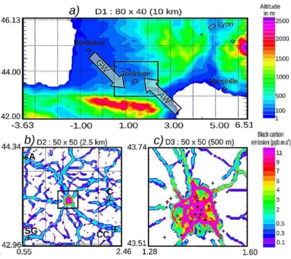
The CAPITOUL campaign took place from February 2004 to February 2005 in the city of Toulouse, located in southwest France (Masson et al., 2008). Figure 1a shows the location of Toulouse and the elevation levels highlighting the wind corridor from

5

northwest to southeast. The two arrows represent the prevailing winds which exist over the Toulouse area: the Autan wind (AW) blows from the Mediterranean sea to the northwest, while the general synoptic wind (GW) blows from the Atlantic Ocean to the southeast. The main regional cities with a potential pollution interaction are shown with black contours: Marseille (M) with 1 000 000 inhabitants, Lyon (L) with 1 200 000

10

inhabitants, Bordeaux (B) with 800 000 inhabitants and Toulouse (T) with 860 000 in-habitants. This campaign aimed at studying the urban climate, including the energetic exchanges between the surface and the atmosphere, the dynamics of the boundary layer over the city, and its interactions with aerosol chemistry. In this context the aging of aerosol particles and the interactions between the urban dynamics and the

disper-15

sion of pollutant particles is especially relevant during summer, when the photochem-istry is high and encourages the formation of secondary aerosols. The IOP chosen for this study occurred during Saturday and Sunday (3–4 July 2004), which fell on a holiday week-end with high tra_ffic. The choice of this IOP allows us to study the two main wind regimes which are representative of the dynamical situation in the Toulouse

20

(5)

ACPD

10, 29569–29598, 2010

Title Page

Tables Figures

◭ ◮

Back Close

Full Screen / Esc

Discussion

P

a

per

|

Dis

cussion

P

a

per

|

Discussion

P

a

per

|

Discussio

n

P

a

per

2.2 Model configuration

To perform this numerical study, the research atmospheric model Meso-NH was used. Meso-NH (Lafore et al., 1998) is a non-hydrostatic and anelastic atmospheric model jointly developed by CNRM-GAME (Meteo-France/CNRS) and Laboratoire d’A ´erologie (UPS/CNRS). The turbulence scheme is one dimensional along the vertical axis

5

(Bougeault and Lacarrere, 1989). The surface computations include four main surface schemes: Town Energy Balance (TEB, Masson (2000)) for managing the urban areas, ISBA for the natural and agricultural covers (Noilhan and Planton, 1989), FLAKES for the lakes (Salgado and Moigne, 2010), and a scheme for sea-surface coverage (Fairall et al., 2003). The Town Energy Budget (TEB) scheme is built following the canyon

ap-10

proach, generalized in order to represent larger horizontal scales. The physics treated by the scheme is relatively complete. Due to the complex shape of the city surface, the urban energy budget is split into different parts: three surface energy budgets are con-sidered: one for the roofs, one for the roads, and one for the walls. Orientation effects are averaged for roads and walls. In addition to the meteorological variables, Meso-NH

15

computes the gaseous chemistry evolution and solves the aerosol equilibrium at each time step and on each grid point (Tulet et al., 2003). The chemical reaction module employs an 82 species: ReLACS2 (Reduced Lumped Atmospheric Chemical Scheme 2) scheme (Tulet et al., 2005) based on the CACM (Caltech Atmospheric Chemistry Mechanism) scheme developed by Griffin et al. (2002). The aerosol particle

mod-20

ule, ORILAM-SOA (Organic Inorganic Lognormal Aerosol Model including Secondary Organic Aerosol) (Tulet et al., 2005, 2006) drives the thermodynamical equilibrium be-tween gases and particles along the MPMPO (Model to Predict the Multiphase Parti-tioning of Organics) scheme (Griffin et al., 2002) for organic species and the scheme EQSAM (EQuilibrium Simplified Aerosol Module) (Metzger et al., 2002) for inorganic

25

(6)

ACPD

10, 29569–29598, 2010

Title Page

Tables Figures

◭ ◮

Back Close

Full Screen / Esc

Discussion

P

a

per

|

Dis

cussion

P

a

per

|

Discussion

P

a

per

|

Discussio

n

P

a

per

|

– black carbon (BC) and primary organic carbon (OC_p) for the primary species

– NO−₃, SO2₄−, NH+₄ for the inorganic ions

– 10 classes of secondary organic aerosol (SOA1,...,10) from Griffin et al. (2002)

– water (H₂O)

The configuration used for the simulations is made of three nested domains

rep-5

resented in Fig. 1. The black squares on the first and second domain represent the second and third domain location, respectively. The first domain covers 800 km by 400 km with a 10 km resolution. The second domain centered on the city of Toulouse represents a 125 by 125 km2square with a 2.5 km resolution. The third domain has a 500 m resolution and covers a 25 km by 25 km area centered on downtown Toulouse.

10

The vertical axis has a 62-level non-linear resolution, from 10 m above ground level to 1 km above 10 km. To initialize the 2-day simulation, a 2-day spin-up is performed. During this 2-day spin-up, the first day is performed only with the first domain and the second day with the first and the second domains. The regional forcing and initialisa-tion are driven by ARPEGE re-analysis for the dynamics and MOCAGE for the gaseous

15

initialisation. For particles, the background aerosols have been set up by deriving the CO concentration (Cachier et al., 2005).

2.3 Emission inventory

In order to have a correct representation of the gas-phase chemistry and the aerosol particle concentrations, an emission inventory of particles and gases has been made.

20

For that purpose, road locations,traffic information during the IOP, and calculations from COPERT-4 software (Ntziachristos et al., 2009) are merged to perform a 500-m resolution e500-mission inventory over the third do500-main. This horizontal resolution is needed to be consistent with the horizontal resolution of the model. The COPERT-4 software is used for the computation of the averaged emissions for the major gases and

(7)

ACPD

10, 29569–29598, 2010

Title Page

Tables Figures

◭ ◮

Back Close

Full Screen / Esc

Discussion

P

a

per

|

Dis

cussion

P

a

per

|

Discussion

P

a

per

|

Discussio

n

P

a

per

particles over a year with the statistical data of French road traffic as an input. Then the emissions are scaled for one vehicle. Finally the tra_ffic counts collected during the 2-day IOP are applied to the previous computation, in order to obtain an hourly emission database of CO, CO2, NOx, SO2, BC and OCp. The VOC (Volatile Organic

Compounds) emissions are deduced by applying a coe_fficient from Matsui et al. (2009)

5

to NOx emissions. Assuming that the main NH3 emissions around Toulouse are not

mainly from traffic emissions but due to agricultural activities, NH3is emitted according

to the GEMS inventory (Visschedijk et al., 2007) with an horizontal resolution of 1₈ degree by ₁₆1 degree.

As an example, Figure 1 shows the emissions of black carbon from this inventory

10

over the second and third domain at 10:00 UTC the 3rd July.

3 Description of the IOP and model results 3.1 Description of the situation

The situation observed and modeled during this two-day IOP has been analyzed both at a meso-scale and at sub-regional scale.

15

3.1.1 Meso scale pollution

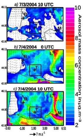
Figure 2 shows the aerosol mass concentrations over the first domain with a horizontal resolution of 10 km at three representative given moments: 3 July at 10:00 UTC, 4 July at 00:00 UTC and 4 July at 10:00 UTC. Figure 2a shows that on 3 July, the synoptic wind blows from northwest over Toulouse (T), Lyon (L) and Marseille (M). The wind

20

(8)

ACPD

10, 29569–29598, 2010

Title Page

Tables Figures

◭ ◮

Back Close

Full Screen / Esc

Discussion

P

a

per

|

Dis

cussion

P

a

per

|

Discussion

P

a

per

|

Discussio

n

P

a

per

|

is mainly out of the boundaries of the domain because of the high wind regime blow-ing from land to sea (>7 m s−1). Figure 2b shows that during the night between 3 and 4 July, the wind velocities stagnate, and especially over the Toulouse area. The plume emitted earlier from Bordeaux reaches the northwest of Toulouse during the night with concentrations of 5 µg m−3as shown in Fig. 2b. The plume originating from

5

Lyon reaches the Mediterranean Sea, 100 km east of Marseille. Then, during the day of 4 July the air flow reverses and the wind blows from southeast over Toulouse. The gas-phase precursors accumulated over Toulouse during the night are mixed with the plume from Bordeaux. In the simulation, the pollution plume emitted on 3 July from Bordeaux reaches an area situated 50 km to the northeast of Toulouse at 00:00 UTC

10

on 4 July when the wind reverses (Fig. 2b). Figure 2c shows the fresh plume from Toulouse almost mixing with the plume emitted from Bordeaux the previous day. The advection of this resulting plume leads to a meeting with a local aerosol concentration maximum located over Bordeaux due to a very low wind regime (<2 m s−1) and the accumulation of particles. The evolution of aerosol mass concentrations as shown in

15

Fig. 2 highlights the regional interactions between different cities. Indeed, the pollution plume developed during 4 July along an axis Toulouse-Bordeaux appears to be a suc-cession of three local maxima resulting from the fresh emissions from Toulouse, the mixing of aerosols emitted by Bordeaux the previous day with secondary aerosols re-sulting from gas-phase emissions by the Toulouse area, and the fresh emissions from

20

Bordeaux respectively. It is also worth noting that in these simulations, the high con-centrations observed on the southern-most part of Fig. 2b and c come from outside the boundary of the domains, and can certainly be attributed to the pollution emitted from Barcelona (Spain).

3.1.2 Sub-regional scale plumes

25

(9)

ACPD

10, 29569–29598, 2010

Title Page

Tables Figures

◭ ◮

Back Close

Full Screen / Esc

Discussion

P

a

per

|

Dis

cussion

P

a

per

|

Discussion

P

a

per

|

Discussio

n

P

a

per

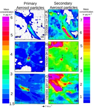
moderate wind (more than 6 m s−1) blows from northwest over Toulouse. Figure 3a describes this situation at 10:00 UTC on 3 July. Primary aerosol concentrations (left) are concentrated over Toulouse (T) where they are emitted with a maximum of mass concentration of 4 µg m−3. Regional cities such as Agen (A), Castres (C), Carcassonne (CC) and Saint-Gaudens (SG) also exhibit local maxima of primary aerosols. The

5

secondary aerosol particles are concentrated along the plume where the gas-phase precursors needed for the photo-reactions are located. The maximum of the secondary aerosols concentration is located 30 km southeast of Toulouse with a value of 7 µg m−3. During the night a low-wind regime develops with mean wind velocities values about 2 m s−1 and a maximum of 4 m s−1. Moreover, on the northwestern-most section of

10

the domain (point A, on Fig. 3b) one can observe a confluence of winds from south, east and northwest. This phenomena leads to an accumulation of primary aerosols with concentrations higher than 6 µg m−3 located over Toulouse as shown on Fig. 3b (left). The secondary aerosol concentrations (right) are quite high (6 µg m−3) on the northwest area of Toulouse (A) due to the resulting plume from Bordeaux created on 3

15

July, and stopped over A during the night because of the low wind regime. Moreover, subsidence, which appeared during the night, brings the aerosols located within the mixing layer to the ground, resulting a relatively high secondary aerosol concentration. The minimum value is 3 µg m−3and is located on the southeast part of the 2nd domain in an area not influenced by the plume from Bordeaux. Finally, from 4 July, 06:00 UTC,

20

(not shown here) to the end of the period, the wind reverses and blows from southeast with typical speed of 6 m s−1. As shown in Fig. 3c, on 4 July at 10:00 UTC, the primary aerosols are again concentrated over Toulouse, where they are emitted, with a maxi-mum of 7 µg m−3. The secondary aerosol concentrations are high (>7 µ g m−3) in the Toulouse plume due to the high concentrations of gas-phase precursors accumulated

25

(10)

ACPD

10, 29569–29598, 2010

Title Page

Tables Figures

◭ ◮

Back Close

Full Screen / Esc

Discussion

P

a

per

|

Dis

cussion

P

a

per

|

Discussion

P

a

per

|

Discussio

n

P

a

per

|

3.2 Urban scale simulations analysis

The model results at local scale have been evaluated in regard to observations. The dynamics and aerosol evolution are both compared to measurements.

3.2.1 Evolution of the wind profile

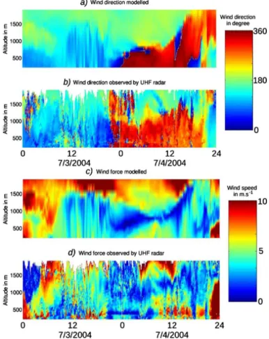
Figure 4 represents the modeled (a) and observed (b) evolution of the wind direction ,

5

and the modeled (c) and observed (d) wind speed during the 48 hours of the simula-tion. Observations were carried out with an UHF radar located in Toulouse downtown (Masson et al., 2008). Figure 4 allows us to focus on the di_fferent wind regimes ob-served over Toulouse and compare them with the simulation results. Figure 4a and 4b show that the wind direction on 3 July (plotted in light blue colors) is from northwest

10

as described at the larger model scale (Sect. 2). On 4 July, the observations show a southeast wind (plotted in orange colors) within the mixing layer. The observations also show a wind shear with opposite directions above the boundary layer at 1000 m on 4 July 00:00 UTC and increasing to 2000 m between 12:00 to 18:00 UTC. The wind regimes are correctly represented for the studied period including the shear above the

15

boundary layer itself and the boundary layer height which can be deduced from the altitude of the shear as well. However, some differences also exist between the obser-vations and simulation results. First, during the night, the observed and modeled wind directions above the height of 1000 m are almost opposite. Second, the height of the shear during the night is not the same. From 00:00 to 06:00 UTC, the simulation

rep-20

resents a shear at 700 m height, while the observations show a shear at about 1000 m height.

Figure 4c and d show the modeled and observed evolution of wind velocity pro-files. While the wind direction observations were consistent on, the wind velocities observed are more random. Nevertheless, the observations first show that the wind

25

(11)

ACPD

10, 29569–29598, 2010

Title Page

Tables Figures

◭ ◮

Back Close

Full Screen / Esc

Discussion

P

a

per

|

Dis

cussion

P

a

per

|

Discussion

P

a

per

|

Discussio

n

P

a

per

(<3 m s−1) from 3 July, 22:00 UTC, to 4 July, 06:00 UTC. Model results show the same low wind regime during the night for layers smaller than 1000 m. However, the simula-tion results show that on 4 July, the wind blows back to northwest earlier than observed for lower layers. Moreover, on 3 and 4 July, while the model simulates a wind speed with lower maxima and higher minima, the average is similar to the observations. The

5

average wind speed modeled for 3 July from 06:00 to 20:00 UTC at the ground level is 4 m s−1, compared to 5 m s−1 for the observations. Similarly, for 4 July from 06:00 to 20:00 UTC, the average modeled wind speed at the ground is 5 m s−1, compared to 6m.s−1 for the observations. While the main trend seems to be correctly simulated, the wind speed is slightly underestimated with respect to observations. In general,

10

the model manages to reproduce the main trends for the wind evolution (speed and direction). Most of the di_fferences between observations and model results are below 1 m s−1 for the wind speed and 45 degrees for the direction. Temperature and relative humidity observations from 21 meteorological stations in Toulouse area also were also in relatively good agreement with model results (not shown here).

15

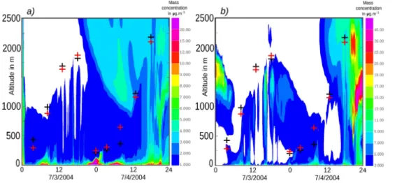
3.2.2 Evolution of aerosol mass concentrations

An other criteria of model evaluation is to examine the modeled aerosol mass concen-trations. Figure 5 shows the evolution of the measurements of (a) black carbon and (b) total aerosol mass concentrations (represented by black crosses) for the downtown site. The dashed red (blue) line shows the evolution of the modeled black carbon (total

20

aerosol) mass concentration for the grid point of the downtown-site, and the red (blue) contour filled by orange (light blue) denotes the minimum and maximum of the modeled concentrations at grid points located in the downtown Toulouse stations which are all located over a 4 by 4 km square centered on the downtown-site. The average values corresponding to this area are drawn in dashed black line.

25

(12)

ACPD

10, 29569–29598, 2010

Title Page

Tables Figures

◭ ◮

Back Close

Full Screen / Esc

Discussion

P

a

per

|

Dis

cussion

P

a

per

|

Discussion

P

a

per

|

Discussio

n

P

a

per

|

is high and even more pronounced for the black carbon mass concentrations. This can be explained by the direct link between black carbon concentrations and the traf-fic emissions. During the night between Saturday 3 July and Sunday 4 July, the ob-served and modeled black carbon concentrations increase, and this can be explained by an increase of tra_ffic on this week-end night. However, the black carbon

concen-5

trations seem to be overestimated by the simulation during the two days, when the observed concentrations are very low, below 1 µg m−3. Moreover the model results show high spatial variability as black carbon concentrations can reach 9 µg m−3 at 4 July 00:00 UTC at the downtown site, whereas some grid points in the 4 by 4 km area show concentrations below 1 µg m−3. Those temporal and spatial variabilities can also

10

be noticed on the total mass concentrations with a maximum value of 55 µg m−3 and minimum value of 6 µg m−3.

Figure 6 shows the evolution of (a) primary and (b) secondary aerosol mass con-centration profiles over the downtown-site during the 2-day simulation. The boundary layer height observed by balloon measurements is overlaid with black crosses, and the

15

height computed in the simulation is drawn with red crosses. Figure 6 confirms that the boundary layer height is acceptably well represented by the model. However, the height of the mixing boundary layer shows a consistent underestimation (with a diff er-ence between 50 and 200 meters), except on 4 July 08:00 UTC when simulations and observation show heights of 600 m and 300 m, respectively. Figure 6 highlights the

20

difference of vertical distributions between primary and secondary aerosols. Primary aerosols are mainly concentrated at surface, whereas secondary aerosols vertical dis-tribution is more chaotic. Figure 6 also shows the temporal and vertical variability between primary and secondary aerosols, and illustrate that primary aerosol are con-centrated when the emissions are the highest, i.e. when during episodes of high traffic:

25

(13)

ACPD

10, 29569–29598, 2010

Title Page

Tables Figures

◭ ◮

Back Close

Full Screen / Esc

Discussion

P

a

per

|

Dis

cussion

P

a

per

|

Discussion

P

a

per

|

Discussio

n

P

a

per

20:00 UTC. On 4 July 02:00 UTC, the observations show a similar peak of black car-bon resulting in a maximum of mass concentration of 4.5 µg m−3. While this peak is not represented by the simulation, we attribute this difference to observed and simulated meteorology; observations show a change in the wind field at 06:00 UTC (Fig. 4), while the model simulate this change at 02:00 UTC. Another peak of black carbon emission

5

is on 4 July 06:00 UTC with a resulting maximum of Black Carbon mass concentration of 4.5 µg m−3. This peak is correctly represented by the model, and probably results from morning traffic linked with a low mixing layer, as shown with black and red crosses on Fig. 6. We can also notice a mass of primary aerosols reaching Toulouse from 4 July at 10:00 UTC between 1200 and 200 m. Finally, at the end of 4 July, a highly

10

concentrated secondary aerosol air mass reaches Toulouse first 2000 m above the sur-face and followed by mixing throughout the column. The simulation shows that this air mass comes from the Mediterranean coast and is advected over Toulouse with high concentrations of nitrates.

4 Development of the two different pollutants dispersion regimes

15

While it is critical to know the dynamical situation for the understanding and forecasting of pollutant dispersion, it is natural to wonder if the model can reproduce complex situations as convective rolls.

4.1 Evolution of the dynamical parameter−_LHBL MO

Observations such as the wind direction or the potential temperature illustrate that the

20

dynamical situation over Toulouse is very different between the two days of simulation, as the potential temperature differs by 10 K between 3 and 4 July. To focus on those two different situations, Figure 7 represents the evolution of the parameter−HBL

L_MO, where

(14)

ACPD

10, 29569–29598, 2010

Title Page

Tables Figures

◭ ◮

Back Close

Full Screen / Esc

Discussion

P

a

per

|

Dis

cussion

P

a

per

|

Discussion

P

a

per

|

Discussio

n

P

a

per

|

The Monin-Obukhov length is a characteristic length of the stability of the boundary layer, and is expressed asL_MO=u∗

3_θρc

p

κ gH with u∗ the friction velocity, θ the potential

temperature,ρthe air density, cpthe air capacity,κ the Von Karmann constant,g the

gravity acceleration, andH the sensible heat flux. The evolution of the parameter−_LHBL

MO is deduced from observations at two sites (Fig. 7

5

in blue over the downtown site of Toulouse and in green over the Saint-Sardos site located 30 km northwest of Toulouse) and during the two days of the IOP (in continuous line for 3 July and in dashed line for the 4 July) Many experimental and modelling studies have characterized the behaviour of the boundary layer as a function of the parameter−_LHBL

MO. Grossman (1982) describes the function of the parameter value as

10

follows:

– −_LHBL MO

≤5.0: Only roll vortex motion

– −_LHBL

MO≤7.3: Rolls coexist with convective cells and are necessary for their mainte-nance; rolls dominant

– 7.3≤ −_LHBL

MO≤21.4: Rolls coexist with convective cells but are not necessary for

15

their maintenance; random cells dominant

– 21.4≤ −_LHBL

MO: Random cells only but the shear is important to cell structure and morphology

Those values are deduced from the BOMEX campaign over the ocean. Other stud-ies (Weckwerth, 1994; Moeng and Sullivan, 1994; Hartmann et al., 1997) suggested

20

other criteria, but the trend is always the same with higher values of−_LHBL

MO representing conditions where convective cells dominate. Although most of these studies show the limits of−_LHBL

MO between 10 and 30 for the separation between cells and rolls, Christian and Wakimoto (1989) observed rolls over Colorado with a value of 270 for−_LHBL

(15)

ACPD

10, 29569–29598, 2010

Title Page

Tables Figures

◭ ◮

Back Close

Full Screen / Esc

Discussion

P

a

per

|

Dis

cussion

P

a

per

|

Discussion

P

a

per

|

Discussio

n

P

a

per

Thus, Figure 7 shows that the dynamical structure over Toulouse area is different between the 2 days of simulation, and the parameter −_LHBL

MO shows values on 4 July lower than those on 3 July at the two observation sites. Moreover observations from the Toulouse site on 4 July (drawn in continuous blue line) has values of−HBL

L_MO most

often lower than 20, which is a commonly observed value for the rolls. Therefore, we

5

could expect the formation of rolls on 4 July.

As previously shown, the plume of particles is represented at the regional scale, by the formation of secondary aerosols in the plume of main cities such as Toulouse. However, with high resolution modelling, the distribution of aerosol particles shows a different shape. This differences are mainly due to effect of the resolution on the

10

turbulent scheme used in the 2nd and 3rd domains. To understand the importance of turbulence regime for the particle dispersion, we focus on the dynamical conditions during the two days of the IOP.

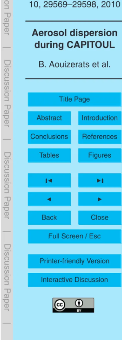
4.2 First day: classic plume of pollution with convective cells

Figure 8 shows a set of 4 instantaneous fields at 12:00 UTC on 3 July. First, the

15

horizontal cross section of the total aerosol mass concentration at 200m above ground level over the 2nd domain is shown in Fig. 8a. The concentrations present a classic plume pattern, with a local maximum of 6 µg m−3 assumed to be primary aerosols as shown in Fig. 3 over the urban area of Toulouse, and 10 µg m−3for aerosols, assumed to be secondary as shown in Fig. 3, 25 km southeast of Toulouse. The horizontal wind

20

vectors are overlaid with black arrows.

Figure 8b presents the same field over the 3rd domain. Unlike over the 2nd domain, the concentrations seem to be concentrated along rolls. Those concentrations show a factor three in and out of the roll (from 4 to 12 µg m−3).

Figure 8c shows the volume of primary aerosol mass concentration equals to

25

(16)

ACPD

10, 29569–29598, 2010

Title Page

Tables Figures

◭ ◮

Back Close

Full Screen / Esc

Discussion

P

a

per

|

Dis

cussion

P

a

per

|

Discussion

P

a

per

|

Discussio

n

P

a

per

|

are advected only along roll motion, the 3-D volume shows cell structures, which seem to concentrate a large amount of particles (eastern part of the Fig. 8c).

Figure 8d shows the vertical cross section of the red line in Figures 8b and 8c for the primary aerosol mass concentration. The convective cells show a mixing height of 1800 m with primary aerosol concentrations of about 6 µg m−3and wind speeds along

5

the vertical cross section higher than 30 m s−1. These wind speeds include a dilatation factor for the vertical wind component equals to 13. This suggest that for a vertical wind arrow along the cross section corresponding to a value of 26 m s−1, the corrected value is 2 m s−1.

Figure 8 illustrates results expected by the observations of the parameter−_LHBL MO, i.e.

10

coexisting cells and rolls. However, the model cannot reproduce those structures with a 2.5 km resolution. Only the 3rd domain with the 500 m resolution manages to reproduce this complex dynamical situation.

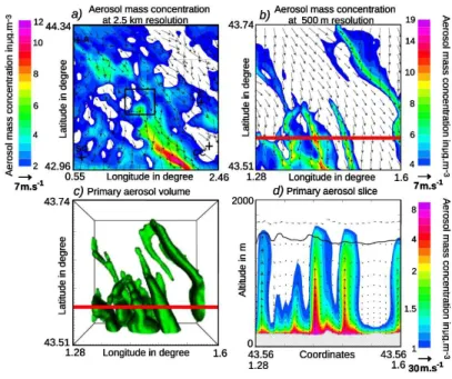
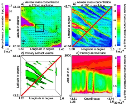
4.3 Second day: turbulent rolls as pollutants drivers

Figure 9 shows the same set of 4 instantaneous fields on 4 July at 12:00 UTC.

Fig-15

ure 9a also shows the horizontal cross section of the total aerosol mass concentration at 200m above ground level over the 2nd domain (as in Fig. 8a). The concentrations still present a classic plume pattern with the concentration of aerosols, assumed to be sec-ondary as shown in Fig. 3,higher than 12 µg m−3located 25 km northwest of Toulouse. The horizontal wind vectors are overlaid with black arrows. Figure 9b presents the

20

same field over the 3rd domain. The rolls are again modeled at 500-m resolution, and represent a more coherent structure. The difference between concentrations located in and out of the rolls is still higher than on 3 July, with values of 15 µg m−3and 4 µg m−3 only separated by only 3 km.

Figure 9c shows the volume of primary aerosol mass concentration equals to

25

(17)

ACPD

10, 29569–29598, 2010

Title Page

Tables Figures

◭ ◮

Back Close

Full Screen / Esc

Discussion

P

a

per

|

Dis

cussion

P

a

per

|

Discussion

P

a

per

|

Discussio

n

P

a

per

Figure 9d shows the vertical cross section (presented as a red line i Figures 9b and 9c) of the primary aerosol mass concentration. In this cross section, only rolls are present. The main differences between 3 July and 4 July is the vertical wind velocities, which are much smaller in the rolls on 4 July (≤0.5 m s−1) than within the convective cells on 3 July (≥2 m s−1). Consequently, the aerosol particles are less mixed within the

5

boundary layer on 4 July even though the potential temperature is 10 K warmer than 3 July. The boundary layer height on 4 July from 10:00 to 18:00 UTC is 250 m less than on 3 July. We can also notice the presence of an highly aerosol concentrated layer above the boundary layer.

Figure 9 illustrates results expected by the observations of the parameter−_LHBL MO, i.e.,

10

only convective rolls are present. However, even when only rolls are present, the model still cannot reproduce those structure with a resolution of 2.5 km. Only the 3rd domain with a resolution of 500 m manages to reproduce this complex dynamical situation.

5 Conclusions

To have a better understanding of the urban meteorological processes, necessary for

15

air quality monitoring, measurements acquired during the CAPITOUL field experiment allowed us to evaluate the performance of high resolution numerical simulations. One of the main sources of uncertainties in air quality forecasting results from representa-tion of the meteorological condirepresenta-tions. Yet the meteorological fields strongly depend on the resolution of the domains. In this study, the importance of the horizontal resolution

20

has been highlighted for adequate representation of the meteorological fields, and the link between the domain resolution and the kind of pollution investigated. While the 10 km resolution domain allows us to focus on pollution events and interaction cities on a regional scale, the 500-m resolution domain permits to investigate the role of boundary layer structure in determining the distribution of pollutant. Both dynamical

25

(18)

ACPD

10, 29569–29598, 2010

Title Page

Tables Figures

◭ ◮

Back Close

Full Screen / Esc

Discussion

P

a

per

|

Dis

cussion

P

a

per

|

Discussion

P

a

per

|

Discussio

n

P

a

per

|

these two days, the turbulent situation was different with convective rolls concentrating the major part of the aerosol particles. The impact of this roll structure is highlighted by a factor of 5 of the pollutant concentration that can be observed over distances shorter than 3 km. Consequently, this study illustrates the importance in reproducing such structures in case of local pollution event or chemical accident. The suggested high

5

sensitivity of roll structures to dynamical situation should be further investigated; in par-ticular, the feedbacks of aerosol particles on atmospheric dynamics through radiative forcing.

Acknowledgements. The authors are indebted to Valery Masson for the organization of the CAPITOUL experiment. They gratefully thank Meteo France for its support. Logistic help from

10

local agencies (La Poste, ORAMIP) is gratefully acknowledged. The authors would also like to thank G. Roberts for its valuable comments on this paper.

The publication of this article is financed by CNRS-INSU.

15

References

Aiken, A. C., de Foy, B., Wiedinmyer, C., DeCarlo, P., Ulbrich, I., Wehrli, M., Szidat, S., Prevot, A., Noda, J., Wacker, L., Volkamer, R., Fortner, E., Wang, J., Laskin, A., Shutthanandan, V., Zheng, J., Zhang, R., Paredes-Miranda, G., Arnott, W., Molina, L., Sosa, G., Querol, X., and Jimenez, J.: Mexico city aerosol analysis during MILAGRO using high resolution

20

(19)

ACPD

10, 29569–29598, 2010

Title Page

Tables Figures

◭ ◮

Back Close

Full Screen / Esc

Discussion

P

a

per

|

Dis

cussion

P

a

per

|

Discussion

P

a

per

|

Discussio

n

P

a

per

Baklanov, A., H ¨anninen, O., Slørdal, L. H., Kukkonen, J., Bjergene, N., Fay, B., Finardi, S., Hoe, S. C., Jantunen, M., Karppinen, A., Rasmussen, A., Skouloudis, A., Sokhi, R. S., Sørensen, J. H., and Ødegaard, V.: Integrated systems for forecasting urban meteorology, air pollution and population exposure, Atmos. Chem. Phys., 7, 855–874, doi:10.5194/acp-7-855-2007, 2007. 29570

5

Bessagnet, B., Menut, L., Curci, G., Hodzic, A., Guillaume, B., Liousse, C., Moukhtar, S., Pun, B., Seigneur, C., and Schulz, M.: Regional modeling of carbonaceous aerosols over Europe – Focus on Secondary Organic Aerosols, J. Atmos. Chem., in press, 2009. 29571

Bougeault, P. and Lacarrere, P.: Parametrization of orography-induced turbulence in a meso-beta model, Mon. Weather Rev., 117, 1872–1890, 1989. 29573

10

Brown, L.: Eco-Economy: Building an Economy for the Earth, New York & London: Earth Policy Institute & W.W. Norton & Company. 2001. 29570

Cachier, H., Aulagnier, F., Sarda, R., Gautier, F., Masclet, P., Besombes, J., Marchand, N., Despiau, S., Croci, D., Mallet, M., Laj, P., Marinoni, A., Deveau, P., Roger, J., Putaud, J., van Dingenen, R., Dell’Acqua, A., Viidanoja, J., dos Santos, M. M., Liousse, C., Cousin,

15

F., Rosset, R., Gardrat, E., and Galy-Lacaux, C.: Aerosol studies during the ESCOMPTE Experiment : an overview, Atmos. Res., 74, 547–563, 2005. 29574

Christian, T. and Wakimoto, R.: The relationship between radar reflectivities and clouds associ-ated with horizontal roll convection on 8 August 1982, Mon. Weather Rev., 117, 1530–1544, 1989. 29582

20

Cubison, M. J., Alfarra, M., Allan, J., Bower, K., Coe, H., McFiggans, G., Whitehead, J., Williams, P., Zhang, Q., Jimenez, J., Hopkins, J., and Lee, J.: The characterisation of pollu-tion aerosol in a changing photochemical environment, Atmos. Chem. Phys., 6, 5573–5588, doi:10.5194/acp-6-5573-2006, 2006. 29571

Fairall, C., Hare, J. E., Grachev, A. A., and Edson, J. B.: Bulk parameterization of air-sea fluxes:

25

Updates and verification for the COARE algorithm, J. Climate, 16, 571–591, 2003. 29573 Gomes, L., Mallet, M., Roger, J., and Dubuisson, P.: Effects of the physical and optical

proper-ties of urban aerosols measured during the CAPITOUL summer campaign on the local direct radiative forcing, Meteorol. Atmos. Phys., 108, 289–306, 2008. 29572

Gri_ffin, R., Dabdub, D., and Seinfeld, J.: Secondary organic aerosol. 1. Atmospheric chemical

30

mechanism for production of molecular constituents, J. Geophys. Res., 107(D17), 4332, doi:10.1029/2001JD000 541, 2002. 29573, 29574

(20)

ACPD

10, 29569–29598, 2010

Title Page

Tables Figures

◭ ◮

Back Close

Full Screen / Esc

Discussion

P

a

per

|

Dis

cussion

P

a

per

|

Discussion

P

a

per

|

Discussio

n

P

a

per

|

Urban Scale Modellinge, CAC: An Air Pollution Model from Regional to Urban Scale Mod-elling, edited by Baklanov, A., Mahura, A., and Sokhi, R., Copenhagen, Denmark, 128–134, 2007. 29571

Grossman, R.: An analysis of vertical velocity spectra obtained in the BOMEX fair-weather, trade-wind boundary layer, Bound.-Layer Meteorol., 23, 323–357, 1982. 29582

5

Hartmann, J., Kottmeier, C., and Raasch, S.: Roll vortices and boundary layer development during a cold air outbreak, Bound.-Layer Meteorol., 84, 45–65, 1997. 29582

Lafore, J., Stein, J., Asencio, N., Bougeault, P., Ducrocq, V., Duron, J., Fischer, C., Hereil, P., Mascart, P., Pinty, V. M. J., Redelsperger, J., Richard, E., and de Arellano, J. V.-G.: The Meso-NH atmospheric simulation system. PArt I: adiabatic formulation and control

simula-10

tions, Ann. Geophys., 16, 90–109, 1998,

http://www.ann-geophys.net/16/90/1998/. 29573

Lefvre, F., Brasseur, G., Folkins, I., Smith, A., and Simon, P.: Chemistry of the 1991–1992 stratospheric winter: three-dimensional model simulations, J. Geophys. Res., 99(D4), 8183– 8195, 1994. 29571

15

Masson, V.: A physically-based scheme for the urban energy balance in atmospheric models, Bound.-Layer Meteorol., 94, 357–397, 2000. 29573

Masson, V., Gomes, L., Pigeon, G., Liousse, K., Lagouarde, J.-P., Voogt, J., Salmond, J., Oke, T., Legain, D., Garrouste, O., and Tulet, P.: The Canopy and Aerosol Particles Interactions in TOulouse Urban Layer (CAPITOUL) experiment, Meteorol. Atmos. Phys., 102(3–4), 135–

20

157, doi:10.1007/s00703-008-0289-4, 2008. 29571, 29572, 29578

Matsui, H., Koike, M., Takegawa, N., Kondo, Y., Griffin, R. J., Miyazaki, Y., Yokouchi,

Y., and Ohara, T.: Secondary organic aerosol formation in urban air: Temporal varia-tions and possible contribuvaria-tions from unidentified hydrocarbons, J. Geophys. Res., 114, D04201,doi:10.1029/2008JD010164, 2009. 29575

25

Metzger, S., Dentener, F., Pandis, S., and Lelieveld, J.: Gas/aerosol partitioning: 1. A compu-tationally efficient model, J. Geophys. Res., 107, ACH16.1–ACH16.24, 2002. 29573

Moeng, C. and Sullivan, P.: A comparison of shear and boyancy driven planetary boundary layer flows, J. Atmos. Sci., 51, 999–1022, 1994. 29582

Noilhan, J. and Planton, S.: A simple parameterization of land surface processes for

meteoro-30

logical models, Mon. Weather Rev., 117, 536–549, 1989. 29573

(21)

ACPD

10, 29569–29598, 2010

Title Page

Tables Figures

◭ ◮

Back Close

Full Screen / Esc

Discussion

P

a

per

|

Dis

cussion

P

a

per

|

Discussion

P

a

per

|

Discussio

n

P

a

per

504, doi:10.1007/978-3-540-88351-7 37, 2009. 29574

Salgado, R. and Moigne, P. L.: Coupling of the FLake model to the Surfex externalized surface model, Boreal Environ. Res., 15(2), 2010. 29573

Smith, S. and Mueller, S. F.: Modeling natural emissions in the Community Multiscale Air Quality (CMAQ) Model – I: building an emissions data base, Atmos. Chem. Phys., 10, 4931–4952,

5

doi:10.5194/acp-10-4931-2010, 2010. 29571

Tulet, P., Crassier, V., Solmon, F., Guedalia, D., and Rosset, R.: Description of the

MESOscale NonHydrostatic Chemistry model and application to a transboundary pollution episode between northern France and southern England, J. Geophys. Res., 108(D1), 4021, doi:10.1029/2000JD000301, 2003. 29573

10

Tulet, P., Crassier, V., Cousin, F., Shure, K., and Rosset, R.: ORILAM, A three moment lognor-mal aerosol scheme for mesoscale atmospheric model. On-line coupling into the MesoNH-C model and validation on the ESMesoNH-COMPTE campaign, J. Geophys. Res., 110, D18201, doi:10.1029/2004JD005716, 2005. 29573

Tulet, P., Grini, A., Griffin, R., and Petitcol, S.: ORILAM-SOA: A computationally efficient model

15

for predicting secondary organic aerosols in 3D atmospheric models., J. Geophys. Res., 111, D23208, doi:10.1029/2006JD007152, 2006. 29573

Visschedijk, A., Zandveld, P., and van der Gon, H.: A High Resolution Gridded European Emission Database for the EU Integrated Project GEMS, Technical Report TNO, aR0233/B, TNO, Apeldoorn, 2007. 29575

20

(22)

ACPD

10, 29569–29598, 2010

Title Page

Tables Figures

◭ ◮

Back Close

Full Screen / Esc

Discussion

P

a

per

|

Dis

cussion

P

a

per

|

Discussion

P

a

per

|

Discussio

n

P

a

per

|

Fig. 1.The three nested domains color-coded for(a)elevation above sea level in meter,(b)and

(c)and black carbon emissions in ppb m s−1at 3 July 10:00 UTC. In(a)the arrows symbolize the two dominant wind regimes AW for the Autan wind and GW for the general wind. The black crosses over the 2nd domain (b) mark the main regional cities: A for Agen, SG for

Saint-Gaudens, CC for Carcassonne, and C for Castres. The crosses over the 3rd(c)domain denote

(23)

ACPD

10, 29569–29598, 2010

Title Page

Tables Figures

◭ ◮

Back Close

Full Screen / Esc

Discussion

P

a

per

|

Dis

cussion

P

a

per

|

Discussion

P

a

per

|

Discussio

n

P

a

per

Fig. 2. Aerosol mass concentrations in µg m−3

(color scale) over the 1st domain(a)on 3 July

10:00 UTC ,(b) on 4 July 00:00 UTC, (c) on 4 July 10:00 UTC with the wind vectors at the

(24)

ACPD

10, 29569–29598, 2010

Title Page

Tables Figures

◭ ◮

Back Close

Full Screen / Esc

Discussion

P

a

per

|

Dis

cussion

P

a

per

|

Discussion

P

a

per

|

Discussio

n

P

a

per

|

Fig. 3. Primary (left) and secondary (right) aerosol mass concentrations in µg m−3 over the

second domain(a)on 3 July 10:00 UTC,(b)on 4 July 00:00 UTC and(c)on 4 July 10:00 UTC

(25)

ACPD

10, 29569–29598, 2010

Title Page

Tables Figures

◭ ◮

Back Close

Full Screen / Esc

Discussion

P

a

per

|

Dis

cussion

P

a

per

|

Discussion

P

a

per

|

Discussio

n

P

a

per

(26)

ACPD

10, 29569–29598, 2010

Title Page

Tables Figures

◭ ◮

Back Close

Full Screen / Esc

Discussion

P

a

per

|

Dis

cussion

P

a

per

|

Discussion

P

a

per

|

Discussio

n

P

a

per

|

Fig. 5. (a)Black carbon and(b) total aerosol mass concentration in µg m−3

measured (black

crosses) and modeled at the downtown-site in dashed (a) red line and (b) blue lines. The

envelope which encompass all the downtown station measurements are in(a)orange and(b)

(27)

ACPD

10, 29569–29598, 2010

Title Page

Tables Figures

◭ ◮

Back Close

Full Screen / Esc

Discussion

P

a

per

|

Dis

cussion

P

a

per

|

Discussion

P

a

per

|

Discussio

n

P

a

per

(28)

ACPD

10, 29569–29598, 2010

Title Page

Tables Figures

◭ ◮

Back Close

Full Screen / Esc

Discussion

P

a

per

|

Dis

cussion

P

a

per

|

Discussion

P

a

per

|

Discussio

n

P

a

per

|

(29)

ACPD

10, 29569–29598, 2010

Title Page

Tables Figures

◭ ◮

Back Close

Full Screen / Esc

Discussion

P

a

per

|

Dis

cussion

P

a

per

|

Discussion

P

a

per

|

Discussio

n

P

a

per

Fig. 8. (a)aerosol mass concentration over the 2nd domain. (b)aerosol mass concentration over the 3rd domain.(c)volume of primary aerosol mass concentration equals to 1 µg m−3.(d)

(30)

ACPD

10, 29569–29598, 2010

Title Page

Tables Figures

◭ ◮

Back Close

Full Screen / Esc

Discussion

P

a

per

|

Dis

cussion

P

a

per

|

Discussion

P

a

per

|

Discussio

n

P

a

per

|

Fig. 9. (a)aerosol mass concentration over the 2nd domain. (b)aerosol mass concentration over the 3rd domain.(c)Volume of primary aerosol mass concentration equals to 1 µg m−3.(d)