Field determination of biomass burning emission ratios and factors via open-path FTIR spectroscopy and fire radiative power assessment: headfire, backfire and residual smouldering combustion in African savannahs

(1)

ACPD

11, 3529–3578, 2011

Field determination of biomass burning

emission ratios

M. J. Wooster et al.

Title Page

Abstract Introduction

Conclusions References

Tables Figures

◭ ◮

Back Close

Full Screen / Esc

Printer-friendly Version Interactive Discussion

Discussion

P

a

per

|

Dis

cussion

P

a

per

|

Discussion

P

a

per

|

Discussio

n

P

a

per

|

Atmos. Chem. Phys. Discuss., 11, 3529–3578, 2011 www.atmos-chem-phys-discuss.net/11/3529/2011/ doi:10.5194/acpd-11-3529-2011

Atmospheric Chemistry and Physics Discussions

This discussion paper is/has been under review for the journal Atmospheric Chemistry and Physics (ACP). Please refer to the corresponding final paper in ACP if available.

Field determination of biomass burning

emission ratios and factors via open-path

FTIR spectroscopy and fire radiative

power assessment: headfire, backfire and

residual smouldering combustion in

African savannahs

M. J. Wooster1,2, P. H. Freeborn1, S. Archibald3, C. Oppenheimer4,5,6, G. J. Roberts1,2, T. E. L. Smith1, N. Govender7, M. Burton8, and I. Palumbo9

1

King’s College London, Environmental Monitoring and Modelling Research Group, Department of Geography, Strand, London, WC2R 2LS, UK

2

NERC National Centre for Earth Observation, UK

3

Natural Resources and the Environment, CSIR, P.O. Box 395, Pretoria 0001, South Africa

4

Le Studium, Institute for Advanced Studies, Orl ´eans and Tours, France

5

Institut des Sciences de la Terre d’Orl éans, 1a rue de la F érollerie, Orl éans 45071, France

6

Department of Geography, University of Cambridge, Cambridge CB2 3EN, UK

(2)

ACPD

11, 3529–3578, 2011

emission ratios

Title Page

Tables Figures

◭ ◮

Back Close

Full Screen / Esc

Discussion

P

a

per

|

Dis

cussion

P

a

per

|

Discussion

P

a

per

|

Discussio

n

P

a

per

|

7

Scientific Services, Kruger National Park, Private Bag X402, Skukuza, 1350, South Africa

8

Istituto Nazionale di Geofisica e Vulcanologia, Via della Faggiola, 32-56126 Pisa, Italy

9

DG Joint Research Centre, Global Environment Monitoring Unit, Ispra, Italy

Received: 1 August 2010 – Accepted: 6 January 2011 – Published: 1 February 2011 Correspondence to: M. J. Wooster (martin.wooster@kcl.ac.uk)

(3)

ACPD

11, 3529–3578, 2011

emission ratios

Title Page

Tables Figures

◭ ◮

Back Close

Full Screen / Esc

Discussion

P

a

per

|

Dis

cussion

P

a

per

|

Discussion

P

a

per

|

Discussio

n

P

a

per

|

Abstract

Biomass burning emissions factors are vital to quantifying trace gases releases from vegetation fires. Here we evaluate emissions factors for a series of savannah fires in Kruger National Park (KNP), South Africa using ground-based open path Fourier transform infrared (FTIR) spectroscopy and an infrared lamp separated by 150–250 m 5

distance. Molecular abundances along the extended open path are retrieved using a spectral forward model coupled to a non-linear least squares fitting approach. We demonstrate derivation of trace gas column amounts for horizontal paths transecting the width of the advected plume, and find, for example, that CO mixing ratio changes of

∼0.001 µmol mol−1(∼10 ppbv) can be detected across the relatively long optical paths

10

used here. We focus analysis on five key compounds whose production is preferen-tial during the pyrolysis (CH2O), flaming (CO2) and smoldering (CO, CH4, NH3) fire phases. We demonstrate that well constrained emissions ratios for these gases to both CO₂ and CO can be derived for the backfire, headfire and residual smouldering combustion stages of these savannah fires, from which stage-specific emission factors 15

can then be calculated. Headfires and backfires in general show similar emission ratios and emission factors, but those of the residual smouldering combustion stage can di_ffer substantially (e.g., ERCH₄/CO₂ up to∼7 times higher than for the flaming stages). The timing of each fire stage was identified via airborne optical and thermal IR imagery and ground-observer reports, with the airborne IR imagery also used to derive estimates 20

of fire radiative energy, thus allowing the relative amount of fuel burned in each stage to be calculated and the “fire averaged” emission ratios and emission factors to be de-termined. The derived “fire averaged” emission ratios are dominated by the headfire contribution, since the vast majority of the fuel is burned in this stage. Our fire aver-aged emission ratios and factors for CO2 and CH4 agree with those from published 25

studies conducted in the same area using airborne plume sampling, and we concur with past suggestions that emission factors for formaldehyde in this environment ap-pear substantially underestimated in widely used databases. We also find the emission

(4)

ACPD

11, 3529–3578, 2011

emission ratios

Title Page

Tables Figures

◭ ◮

Back Close

Full Screen / Esc

Discussion

P

a

per

|

Dis

cussion

P

a

per

|

Discussion

P

a

per

|

Discussio

n

P

a

per

|

ratios and factors for CO and NH₃to be somewhat higher than most other estimates, however, we see no evidence to support suggestions of a major overestimation in the emission factor of ammonia. Our data also suggest that the contribution of burning animal (elephant) dung can be a significant factor in the emissions characteristics of certain KNP fires, and indicate some similarities between the time series of fire bright-5

ness temperature and modified combustion efficiency (MCE) that supports suggestions that EO-derived fire temperature estimates maybe useful when attempting to remotely classify fire activity into its different phases. We conclude that ground-based, extended open path FTIR spectroscopy is a practical and very effective means for determining emission ratios, emission factors and modified combustion efficiencies at open vegeta-10

tion fire plumes, allowing these to be probed at temporal and spatial scales di_fficult to explore using other ground-based approaches. Though we limited our study to five key emissions products, open path FTIR spectroscopy can detect dozens of other species, as has been demonstrated during previous closed-path FTIR airborne deployments in the same study area.

15

1 Introduction

Alongside the burning of coal, oil and natural gas, the open combustion of biomass in forest and grassland fires is one of the key pathways by which humans directly affect the atmosphere. The gases and particulates released in biomass burning plumes have substantial short- and long-term chemical, radiative and climatic impacts (Bowman et 20

al., 2009) and proper assessment of these effects generally requires spatio-temporally resolved data on the source emissions magnitude and makeup. This information is usually obtained via multiplication of the mass of dry fuel consumed in the fire [M, kg] by an emission factor [EF_x] representing the amount of chemical species (x) released per kg of dry fuel burned (Andreae and Merlet, 2001). In these calculations, the fuel 25

(5)

ACPD

11, 3529–3578, 2011

emission ratios

Title Page

Tables Figures

◭ ◮

Back Close

Full Screen / Esc

Discussion

P

a

per

|

Dis

cussion

P

a

per

|

Discussion

P

a

per

|

Discussio

n

P

a

per

|

(e.g., Korontzi et al., 2004; van der Werf et al., 2006). Satellite-derived Fire Radiative Power (FRP) observations also enable estimation of fuel consumption, being partic-ularly appropriate when fuel loads are very uncertain (e.g., Reid et al., 2009), where combustion rates rather than totals are required (e.g., Roberts et al., 2009), and/or where near real-time information is needed for operational forecast-type applications 5

(e.g., Kaiser et al., 2009; Xu et al., 2010). In all cases, emissions factors are a vital component of the calculation, and since uncertainties in EF_x propagate linearly onto uncertainties in the derived emissions there is a continued requirement for improved EF_x information and for relationships from which estimates of these maybe better con-strained (e.g., Korontzi et al., 2003). This need is increasingly heightened as satellite 10

products related to fuel consumption estimation become more mature (e.g. van der Werf et al., 2006; Roy et al., 2008; Freeborn et al., 2009; Giglio et al., 2009).

At present, the emissions factor for use at a particular fire is usually selected from a published database, commonly that of Andreae and Merlet (2001) and subsequent updates. The estimates of EF_x are derived using a variety of means, commonly via 15

smoke emission ratio measures (ER_x/y, the relative amounts of two smoke species (x) and (y)). As Keene et al. (2006) suggest, emissions ratios (ERs) and emissions factors (EFs) for many species typically show wide variations with the ratio of live to dead fuel, fuel component physical type, and fuel arrangement and moisture, in addition to am-bient environmental conditions and fuel elemental content (e.g., nitrogen and sulphur). 20

For some important species, it has been suggested that changes in fuel and environ-mental conditions may induce variations of 500% or more in emissions factors (e.g., Gri_ffith et al., 1991), but such variability is often not fully expressed in databases which may only report averages and which generally do not differentiate between different combustion styles (e.g., backfires and headfires; Smith and Wooster, 2005). Further-25

more, some databases may only include results from small-scale laboratory experi-ments, whist others focus on airborne “whole plume” sampling. Both approaches offer advantages, but whilst the former may not be fully representative of open vegetation fire conditions, the latter typically cannot be used to sample the individual fire phases

(6)

ACPD

11, 3529–3578, 2011

emission ratios

Title Page

Tables Figures

◭ ◮

Back Close

Full Screen / Esc

Discussion

P

a

per

|

Dis

cussion

P

a

per

|

Discussion

P

a

per

|

Discussio

n

P

a

per

|

or stages, and there can be problems in using airborne ER measurements to derive emissions factors and to sample the residual smouldering combustion (RSC) stage (Andreae and Merlet, 2001; Christian et al., 2007; Yokelson et al., 2003; Bertschi et al., 2003). These potential limitations suggest further methodological developments in biomass burning emissions measurements maybe warranted, something the current 5

work aims to contribute to. Furthermore, many of the controls on EFs also regulate combustion efficiency (the ratio of CO2 to total carbon released in the smoke), whose calculation is usually simplified to one based on CO₂and CO concentration measures alone (the modified combustion efficiency (MCE) of Ward and Radke, 1993). Since emissions ratios of many species are well correlated to MCE (Sinha et al., 2003a), 10

one goal in current biomass burning research is to identify methods for determining the most appropriate MCE, ER and EF measures for use in fires burning under par-ticular environmental conditions and fuel types. Such research will most likely require sampling the fuel, fire, meteorological and emissions characteristics of large numbers of open vegetation fires. Recently Fern ´andez-G ´omez et al. (2011) suggested open 15

path Fourier Transform Infra Red (FTIR) spectroscopy as a potential tool for providing emissions measurements at the site of field-scale open vegetation fires, though their proof-of-concept was confined to a small-scale laboratory setup. An objective of the current work is therefore to evaluate whether ground-based, open path FTIR spec-troscopy conducted at the site of real open vegetation fires can provide the necessary 20

information on “plume integrated” smoke chemistry that is commonly required in many biomass burning studies, and also to assess if the technique allows for the study of intra-fire as well as inter-fire emissions variability. We demonstrate the practicalities of deploying OP-FTIR in so-called “long-path” mode (Gosz et al., 1988), measuring smoke trace gas abundances over pathlengths of hundreds of meters, and we evaluate 25

(7)

ACPD

11, 3529–3578, 2011

emission ratios

Title Page

Tables Figures

◭ ◮

Back Close

Full Screen / Esc

Discussion

P

a

per

|

Dis

cussion

P

a

per

|

Discussion

P

a

per

|

Discussio

n

P

a

per

|

studied fires to be quantified. This allows ER_x/y and EF_x to be determined from the FTIR-derived smoke column abundances retrieved separately for each fire stage, and also through their combination to calculate “fire averaged” quantities. The study was conducted in the savannah environment of Southern Africa, whose fires are annually responsible for perhaps around one quarter of global fire fuel consumption (van der 5

Werf et al., 2003; Roberts et al., 2009; Archibald et al., 2010).

2 Background

2.1 Study of laboratory and open fire plumes

Smoke emission ratios, emissions factors and combustion efficiencies can be deduced from trace gas concentrations measured via a number of approaches. Delmas et 10

al. (1995), Goode et al. (2000), Andreae and Merlet (2001) and Koppmann et al. (2005) include detailed reviews, with laboratory combustion chamber measurements being probably the most common. Here fuel consumption and total gas flux can be accu-rately logged, enabling direct calculation of EF_x for the separate flaming and smoul-dering phases, and calculation of so-called “fire-averaged” values via a weighted mean 15

approach. However, fire characteristics in laboratory-scale experiments can di_ffer from natural behaviour, potentially resulting in EF biases (Delmas et al., 1995; Fern ´andez-G ´omez et al., 2011). Trace gas measurements for open vegetation fires are therefore greatly valued, but can be di_fficult to acquire due to fires hazardous, highly dynamic and sometimes unpredictable nature. Furthermore, in open fires all combustion phases 20

maybe occurring simultaneously, with emissions released into one or more “integrat-ing” plumes. Airborne campaigns sample such plumes and o_ffer many practical and scientific benefits (e.g., Yokelson et al., 1999, 2003; Sinha et al., 2003a, 2003b), but lo-gistics and costs can hinder deployments. Since the relative amount of fuel consumed in each phase of the fire is generally unknown when relying on aircraft observations, it 25

is also assumed that natural mixing provides the appropriate averaging (Andreae and

(8)

ACPD

11, 3529–3578, 2011

emission ratios

Title Page

Tables Figures

◭ ◮

Back Close

Full Screen / Esc

Discussion

P

a

per

|

Dis

cussion

P

a

per

|

Discussion

P

a

per

|

Discussio

n

P

a

per

|

Merlet, 2001). Ground sampling of plumes has most commonly involved canister or grab bag collection and subsequent laboratory analysis. Field-deployed spectroscopic methods potentially avoid the problem of within-canister chemical conversion or wall-loss (Goode et al., 2000; Yokelson et al., 2003), and an FTIR system allows a single instrument to provide the IR spectra from which many gases can be simultaneously 5

and continuously monitored at detection limits of∼5–20 parts per billion or better over ∼100 m pathlengths (Griffith et al., 1991; R. J. Yokelson et al., personal

communica-tion, 1996, 1999). This ability to target multiple gases simultaneously may be critical for discerning intra-fire emissions ratio variability.

2.2 FTIR smoke plume studies

10

FTIR-based vegetation fire smoke studies have usually deployed so-called closed-path/extractive techniques, or open path methods covering relatively short (<1–10 m) distances (e.g., Goode et al., 2000; Yokelson et al., 1996, 1999; Bertschi et al., 2003; Christian et al., 2007; Castro et al., 2007; Fern ´andez-G ´omez et al., 2011). Whilst these studies have been extremely productive, sample representativeness is still a concern, 15

and it can prove hazardous and difficult to sample areas of higher intensity combustion. An alternative strategy is offered by extended (long) open path (OP) geometries, us-ing an FTIR spectrometer and IR source separated by potentially hundreds of meters and positioned such that the advected plume passes through the optical path. Whilst commonly deployed in studies of ambient and polluted air, industrial and volcanic emis-20

sions (e.g., Gosz et al., 1998; Hren et al., 2000; Bacsik et al., 2006; Oppenheimer and Kyle, 2007) extended OP-FTIR seems not to have been exploited at sites of open veg-etation fires since the first demonstration by Griffith et al. (1991). Fern ´andez-G ´omez et al. (2011) suggest the time is right for a re-appraisal of the approach, and here we use an extended OP-FTIR setup to measure multiple gases emitted from African savannah 25

(9)

ACPD

11, 3529–3578, 2011

emission ratios

Title Page

Tables Figures

◭ ◮

Back Close

Full Screen / Esc

Discussion

P

a

per

|

Dis

cussion

P

a

per

|

Discussion

P

a

per

|

Discussio

n

P

a

per

|

3 Methodology

3.1 Study area

We analyse the smoke from four prescribed burns conducted in August 2007 – re-ferred to here as Fires 1 to 4. Fires were conducted in Kruger National Park (KNP), South Africa, whose recent fire history is detailed in Archibald et al. (2010). Fires were 5

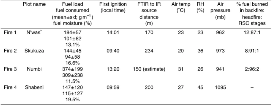
perimeter ignition events conducted towards the peak of the Southern Africa fire sea-son at the KNP long-term experimental burn plots, detailed in Govender et al. (2006). These 7 ha (380 m×180 m) plots were previously used for emissions studies by Ward

et al. (1996), and each had its fuel characteristics and consumption measured via in situ destructive sampling (Table 1). Each plot was first ignited with a backfire (in part to 10

create a larger fire break at the downwind side), followed by headfire ignition some min-utes later at the upwind side. Flaming combustion usually ceased when the headfire reached the downwind plot boundary and/or the area already burnt out by the backfire, typically around 30 min after ignition. On some plots substantial residual smoulder-ing combustion (RSC) continued for tens of minutes after all flamsmoulder-ing activity ceased. 15

Meteorological conditions were logged throughout each burn.

3.2 FTIR measurements

IR spectra were collected using an OP-FTIR Air Monitoring System (MIDAC Corpora-tion, Irvine CA), equipped with a 76 mm Newtonian telescope to deliver a∼9-mrad

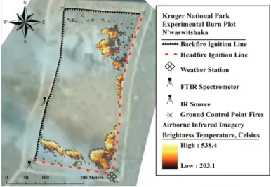
field-of-view and deployed neighbouring each burning plot as shown in Fig. 1. A Stirling-20

cycle cooled mercury-cadmium-telluride (MCT) detector sensitive over the SWIR to TIR spectral range was used to avoid the requirement for liquid nitrogen in the field. The cooled detector, instrument electronics and spectrometer mechanical assemblage were encased in a light, sheet metal casing (size=356×183×166 mm; mass∼9.5 kg)

powered by a 12 V battery and controlled by a laptop computer through a dedicated 25

PCMCIA interface. This detection system was tripod mounted at head height and

(10)

ACPD

11, 3529–3578, 2011

emission ratios

Title Page

Tables Figures

◭ ◮

Back Close

Full Screen / Esc

Discussion

P

a

per

|

Dis

cussion

P

a

per

|

Discussion

P

a

per

|

Discussio

n

P

a

per

|

targeted at a battery powered IR source comprising a tripod-mounted 1275◦

C silicon carbide glower located at the focus of a∼50 cm gold plated aluminium reflector. The

spectrometer and IR source were positioned slightly downwind of the plot, and sep-arated by ∼150–250 m such that the horizontally advected plume filled a significant

fraction of the intervening path (Fig. 2). Longer optical paths were theoretically pos-5

sible, but in practice were blocked by trees and undulating terrain. Nevertheless, the extended pathlengths achieved meant that the quantity of smoke being advected into the optical path was sufficient to completely obscure the IR source when viewed with the naked eye from the detector location (as demonstrated in Fig. 1). We recorded raw interferograms (IFGs) at the highest available spectral resolution (0.5 cm−1

), with 8 10

consecutive scans stacked to improve S/N resulting in an 8-s acquisition time step.

3.3 FRP measurements

During each fire, a GPS-equipped helicopter hovered some hundreds of meters above and slightly to the side of each plot, enabling aerial recording of each fire event over the entire plot area. An AGEMA-550 middle infrared (MIR) thermal imager was used 15

to record the fires radiant energy emission signature across a 320×240 pixel imaging

array. A narrowband filter centred at 3.9 µm was fitted to prevent detector saturation over high intensity fire pixels. Mean ground pixel size across the 40◦×30◦field-of-view

was 1.5–2.5 m, depending upon flying height, calculated using the viewing distance and angle from the helicopter to the plot as determined from the GPS records. Per-pixel 20

measures of FRP were calculated according to the MIR radiance method of Wooster et al. (2003). For each IR imaging frame, the FRP for each detected fire pixel was summed to provide an instantaneous plot-integrated time-stamped FRP measure. This time-series was generated at 5-s intervals for the entire fire duration. Full details of this processing approach are given in Wooster et al. (2005) and Freeborn et al. (2008). 25

(11)

ACPD

11, 3529–3578, 2011

emission ratios

Title Page

Tables Figures

◭ ◮

Back Close

Full Screen / Esc

Discussion

P

a

per

|

Dis

cussion

P

a

per

|

Discussion

P

a

per

|

Discussio

n

P

a

per

|

smoke plume, and to confirm the timing of the separate combustion stages reported by the ignition team. The backfire and headfire stages of each fire were identified based on the direction of travel of the flaming front in relation to the predominant wind direction, a somewhat similar approach to that previously used to distinguish these stages in satellite imagery (Smith and Wooster, 2005). The RSC stage was simply 5

identified as the period of smoke production after all flaming combustion had ceased.

3.4 Retrieval of trace gas abundances

The co-added IFGs were zero-filled by a factor of 2 and had a Mertz phase correc-tion and triangular apodizacorrec-tion funccorrec-tion applied prior to conversion to single beam (SB) spectra via a Fourier transform (Smith, 1996). This pre-processing was enacted in 10

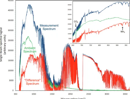
the AutoQuant Pro control and analysis software (MIDAC Corporation, Irvine, CA). Figure 3 shows an example of an SB measurement spectrum collected when view-ing the IR source horizontally through the smoke, together with a “ambient” spectrum collected without the IR source and which is used to ascertain the contribution of in-strument and ambient background emission to the measurement spectra (M ¨uller et al., 15

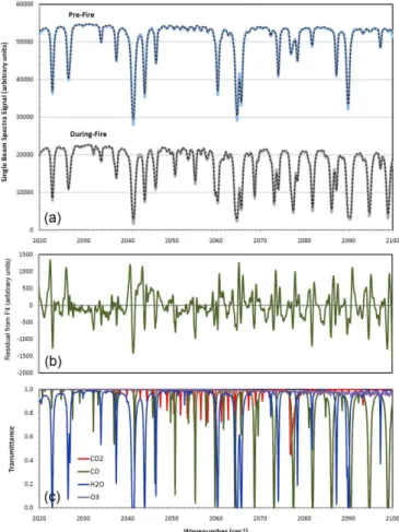
1999). Figure 4 shows examples of pre-fire and during-fire SB measurement spec-tra collected over the specspec-tral window used to retrieve the CO2 and CO (horizontal) column amounts, with the increased absorption features caused by elevated in-plume abundances clearly apparent.

Trace gases within the plume and the ambient atmosphere were identified directly 20

from their spectral signatures in the recorded SB spectra. Briz et al. (2007) provide a detailed review of the methods available to retrieve trace gas column abundances from OP-FTIR spectroscopy data, concluding that approaches based on spectral for-ward models maybe effective in removing the need for a clean “background” spec-trum and avoiding problems with non-linear departures from the Beer-Lambert Law 25

(Childers, 2001). We use such an approach, described in detail by Burton (1998) and Horrocks et al. (2001). The retrieval algorithm is a combination of the Atmospheric Ra-diation Reference Forward Model (RFM v4.0 available at www.atm.ox.ac.uk/RFM/;

(12)

ACPD

11, 3529–3578, 2011

emission ratios

Title Page

Tables Figures

◭ ◮

Back Close

Full Screen / Esc

Discussion

P

a

per

|

Dis

cussion

P

a

per

|

Discussion

P

a

per

|

Discussio

n

P

a

per

|

wards and Dudhia, 1996), the HITRAN 2008 (and updates) spectral database (a com-pilation of spectroscopic parameters for 42 atmospheric molecules; Rothman et al., 2009), the optimal estimation procedure of Rodgers et al. (1976), and the enhanced non-linear fitting procedure of Marquardt (1963). The importance of using an up-to-date version of HITRAN was indicated by the fact that testing with HITRAN 1996 pro-5

duced some emission ratios up to 20% lower than those obtained with the most recent database. These effects should be borne in mind when comparing results from current HITRAN-based FTIR studies to those from prior experiments using older databases.

The retrieval algorithm is parameterized with the atmospheric temperature, pressure, optical path length and the a priori column abundances of the target gases that have 10

absorption features within the spectral window of interest. The transmission of IR radi-ation along the open path is calculated, and a simulated SB spectrum produced. This output is compared to the measured SB spectrum, and a non-linear least squares fitting routine used to optimize the fit by adjusting the assumed trace gas abundances within the simulation. Being similar in design to the widely used SFIT code (Niple et al., 1980; 15

Benner et al., 1995) and the Multiple Atmospheric Layer Transmission model (MALT; Griffith, 1996), the Burton (1998) code has been used in many studies, in particular of volcanic plumes (e.g., Francis et al., 1998; Burton et al., 2000; Oppenheimer and Kyle, 2007). It has been evaluated by Horrocks et al. (2001) to have an absolute ac-curacy of better than 5%, with the uncertainty in the HITRAN spectral line parameters 20

determined to be of a similar magnitude. Yokelson et al. (1996) and Smith et al. (2011) calculated similar accuracies for MALT-based trace gas retrievals during closed-path FTIR studies of both real and simulated biomass burning emissions.

The focus of our work was retrieval of the primary carbonaceous species emitted preferentially during the flaming (CO2), smoldering (CO, CH4) and pyrolysis (CH2O) 25

(13)

ACPD

11, 3529–3578, 2011

emission ratios

Title Page

Tables Figures

◭ ◮

Back Close

Full Screen / Esc

Discussion

P

a

per

|

Dis

cussion

P

a

per

|

Discussion

P

a

per

|

Discussio

n

P

a

per

|

SB spectra, most commonly those measured during periods of higher trace gas col-umn amount. Ammonia, a nitrogenous species emitted primarily in the smouldering phase, was the most readily detected N species, in apparent agreement with Griffith et al. (1991) and Yokelson et al. (1997), and we therefore retrieved NH₃column amounts from all measured spectra. Table 2 lists the spectral windows used for retrieval of 5

each trace gas, where the trace gas(es) of interest possess significant but unsaturated absorption features and where there is limited interference from other species. The “ambient emission” spectrum in Fig. 3, collected without the IR source, confirms that in the higher wavenumber (i.e., shorter wavelength) spectral regions used to retrieve CO₂, CO, CH₄ and CH₂O the signal contribution from instrument self-emission and 10

other ambient temperature sources is minor. Our calculations confirm its e_ffect can be neglected in the retrieval of trace gas column amounts (M ¨uller et al., 1999). However, the lower wavenumber region used to retrieve NH3 lies in the peak spectral emission region for ambient temperature bodies, and Fig. 3 confirms a substantial “ambient” signal at these sub-1000 cm−1wavenumbers. This signal component needs to be re-15

moved from the measurement spectra prior to any trace gas retrieval, since it contains no information on smoke trace gas absorption. We therefore subtracted a relevant ambient SB spectrum from each measurement spectrum, making slight adjustments for MCT detector non-linearities according to M ¨uller et al. (1999) to ensure the resul-tant “di_fference” spectrum showed zero signal in spectral regions expected to be fully 20

opaque, such as the 668–670 cm−1CO2absorption band (Fig. 3 inset).

Figure 4 demonstrates the high quality of the match between our best-fit forward modeled spectral signal and the measured SB spectra, both prior to and during the fire (i.e., “clean air” and “smoke polluted air”). A full error analysis for the Burton (1998) retrieval approach can be found in Horrocks et al. (2001). The FTIR-derived ambient 25

CO₂mixing ratio of 413±6 µmol mol−1(mean±1 s d) calculated on a dry air basis before

Fire 1 from 5 min of 8 s temporal resolution spectrometer data compares reasonably well to the 417±1 µmol mol−1measure provided by a newly calibrated LICOR IR Gas

Analyser. The degree of agreement is of the same order to that found previously by

(14)

ACPD

11, 3529–3578, 2011

emission ratios

Title Page

Tables Figures

◭ ◮

Back Close

Full Screen / Esc

Discussion

P

a

per

|

Dis

cussion

P

a

per

|

Discussion

P

a

per

|

Discussio

n

P

a

per

|

Yokelson et al. (1997) using a similar forward modeling approach. Pre-fire retrievals for the other species examined here were also found to be reasonable.

3.5 Determination of derived trace gas plume metrics

Forward modeling of the measured IR spectra provides the total number of molecules of the target gas species (x) per unit area along the horizontal observation pathlength 5

(molecules cm−2

), here termed the “column amount”. This metric represents the in-tegration of the species abundance in molecules per unit volume along the optical pathlength (l, m). The optical pathlength between the IR source and spectrometer was carefully measured, but the helicopter video record confirms that for most of the fires’ duration only a fraction of the path (f) was filled by plume (see Fig. 2). Therefore 10

the retrieved column amount represents a mixture of ambient air and smoke in un-known relative quantities. Nevertheless, since for each fire the optical path (l) remains constant, the retrieved column amounts do represent the relative proportions of each trace gas present along the path and can thus be used to determine the smoke plume emission ratios, emissions factors and MCE, as detailed below.

15

3.5.1 Emission Ratios (ERs)

The smoke emission ratio [ERx/y] is commonly defined from the gradient of the linear

best fit to the excess abundance of trace gas species (x) when plotted against that of reference species (y) (Yokelson et al., 1999). CO₂is commonly the reference species for “flaming dominant” compounds, and CO for “smoldering dominant” (Andreae and 20

Merlet, 2001). Where ambient reference species concentrations are difficult to obtain, for example where the background air is suspected to already be fire-affected, Guyon et al. (2005) recommend using the gradient of the absolute gas mixing ratios rather than their excess abundances, an approach adopted by Keene et al. (2006). Further-more, since in our OP-FTIR approach the smoke plume typically only partly fills the 25

(15)

ACPD

11, 3529–3578, 2011

emission ratios

Title Page

Tables Figures

◭ ◮

Back Close

Full Screen / Esc

Discussion

P

a

per

|

Dis

cussion

P

a

per

|

Discussion

P

a

per

|

Discussio

n

P

a

per

|

x=l f[X_p]+l(1−f)[X

a] (1)

y =l f[Yp]+l(1−f)[Ya] (2)

where [Xp] and [Yp] are, respectively, the mean molecular volumetric abundances of species (x) and (y) in the pure plume, and [Xa] and [Ya] are the volumetric abun-dances of the same species in the pure ambient atmosphere (all expressed in units 5

of molecules cm−3); and (x) and (y) are, respectively, the total column amounts of these species measured along the optical path (in units of molecules cm−2

); l is the pathlength (here expressed in cm) andf the unitless fraction of the optical path taken up by the pure plume.

Subtracting pre-fire “ambient” abundances from those derived from the during-fire 10

measurements in order to calculate the excess trace gas amounts is therefore not fully correct, since only fraction (1−f) of the optical path contains “clean” air. Fortunately

Eqs. (1) and (2) can be combined to remove dependence on the unknown and variable f:

y= Yp −Y_a

Xp−Xa !

x−l

"

Xa

Yp−Ya Xp−Xa

!

−Y_a

#

(3) 15

Equation (3) is effectively the equation of a straight line (y=mx+c) obtained when the column amount of species (y) is plotted against that of species (x), where the gradient (m) is a function of the relative abundance of the two species in the “pure” plume and “pure” atmosphere:

m= Yp −Y

a

Xp−Xa !

(4) 20

Under the assumption that volumetric abundances of the target species in the pure “unmixed” plume are much greater than those in the pure ambient atmosphere (i.e., Yp≫Ya and Xp≫Xa) thenmapproaches that of the molar emissions ratio of the pure

(16)

ACPD

11, 3529–3578, 2011

emission ratios

Title Page

Tables Figures

◭ ◮

Back Close

Full Screen / Esc

Discussion

P

a

per

|

Dis

cussion

P

a

per

|

Discussion

P

a

per

|

Discussio

n

P

a

per

|

plume (i.e., ERx/y=Yp/Xp). Gases having both high in-plume abundances (CO2∼90% and CO∼6% on a dry air basis according to Andreae and Merlet, 2001) and relatively

low in-plume abundances (CH₄∼0.3% and NH

3∼0.04%) exist in amounts orders of magnitude greater than in the ambient atmosphere, making the gradient (m) equivalent to that of the pure plume ER to within 1%. Hence, as with volcanic plumes (e.g., Sawyer 5

et al., 2008), we can confidently proceed to calculate ERs directly from the retrieved total column amounts.

ER_x/y can vary substantially between different phases, resulting in divergent gradi-ents in the (x) vs. (y) column amount scatter plots (e.g., see examples in Fern ´andez-G ´omez et al., 2011) . Thus phase-specific emission ratios are often calculated, and to 10

calculate the “fire averaged” emission ratio, either the entire amount of species (x) and (y) released in each phase must be measured and ratioed, which is achievable in labo-ratory studies, but impossible for most field setups. Alternatively the weighted average of the instantaneous or phase-specific ER_x/y measures can be calculated using the relative amount of fuel consumed in the relevant time interval. Such fuel consumption 15

data are again relatively easily obtained during laboratory-scale measurements, but are usually unavailable in field situations. However, in the current study the Fire Radia-tive Energy (FRE) data derived from temporal integration of the helicopter-born FRP observations can provide this information. This is because FRE is linearly proportional to fuel consumption, irrespective of whether the fire activity is flaming or smoulder-20

ing, providing the emitter temperature exceeds∼700 K (Wooster et al., 2003, 2005).

It should be noted that whilst the FRE measurements are associated with combustion occurring across the entire plot, the trace gas abundances did not always encompass the full plume width due to the optical path not extending along the complete∼380 m

plot length. Nevertheless, careful inspection of the aerial video record suggests that 25

(17)

ACPD

11, 3529–3578, 2011

emission ratios

Title Page

Tables Figures

◭ ◮

Back Close

Full Screen / Esc

Discussion

P

a

per

|

Dis

cussion

P

a

per

|

Discussion

P

a

per

|

Discussio

n

P

a

per

|

3.5.2 Emission Factors (EFs)

Following Yokelson et al. (1999), Goode et al. (2000), Sinha et al. (2003a) and oth-ers, we calculate the emissions factor for species (x) using the carbon mass balance method of Ward and Radke (1993):

EF_x=Fc1000

MM_x MMcarbon

Cx

C_T (5)

5

Where EFx is the emissions factor for species x (g kg −1

), Fc is the mass fraction of carbon in the fuel (taken here as 0.5±0.05 to be compatible with the majority of other

studies; Ward et al., 1996), MM is the molecular mass of species x (g), 1000 g/kg is a unit conversion factor, MMcarbonis the molecular mass of carbon (12 g), andCx/CT is

the ratio of the number of moles of speciesxin the plume divided by the total number 10

of moles of carbon, calculated as: C_x

CT =

ER_x/_CO

2 n

P

j=1

(NC_jER_j/CO₂)

(6)

Where NC_j is the number of carbon atoms in compound j and the sum is over all carbonaceous species, including CO₂.

As is typical in past studies, not all carbon containing species were quantified in 15

our analysis. Delmas et al. (1995) and Keene et al. (2006) show that CO2 and CO account for the vast majority of the total carbon flux from open biomass burning, a me-dian of around 99% in the case of Southern African savannah fires. The majority of the remaining carbon is emitted as aerosols, and Yokelson et al. (1999) suggest that EFs are underestimated by only 1 or 2% when neglecting these particulates. The car-20

bonaceous gases studied here (CO2, CO, CH4and CH2O) therefore clearly represent almost the total mass of carbon released, and unmeasured trace gases and particu-lates are ignored, which infparticu-lates the derived EFs by a few percent at most (Yokelson et al., 1999; Andreae and Merlet, 2001; Goode et al., 2000).

(18)

ACPD

11, 3529–3578, 2011

emission ratios

Title Page

Tables Figures

◭ ◮

Back Close

Full Screen / Esc

Discussion

P

a

per

|

Dis

cussion

P

a

per

|

Discussion

P

a

per

|

Discussio

n

P

a

per

|

3.5.3 Modified Combustion Efficiency (MCE)

The MCE represents the molar ratio of carbon emitted in the form of CO2to that emitted as CO and CO₂(Ward and Radke, 1993):

MCE= ∆CO2

(∆CO2+ ∆CO)

(7)

where∆CO2 and ∆CO indicate the excess mixing ratio of those species (Ward and 5

Radke, 1993). Linear relationships between species EF_x and MCE were used by Goode et al. (2000) to propose a mechanism to estimate the EFs of unmeasured species in cases where CO and CO2 measures are available, thus highlighting the potential importance of the MCE measure. Our data in theory allow the MCE (and indeed also ERs) to be derived at a very high temporal resolution (i.e., from each SB 10

spectral measurement), though for this it is necessary to base the calculation on ex-cess trace gas abundances rather than the total trace gas column amounts. The MCE for each fire stage can be also be calculated via the relevant ER_CO_/_CO

2 measure using:

MCE= 1

(1+ERCO/CO₂)

(8)

In this work we simply use the MCE measures derived from Eq. (8) as an aid to the 15

interpretation of fire behaviour, rather than to derive other quantities or to separate the individual combustion phases or stages.

4 Results and discussion

4.1 Trace gas and FRP time series

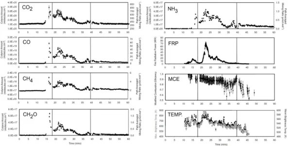
Figure 5 shows the time-series of trace gas column amounts, FRP, MCE and remotely 20

(19)

ACPD

11, 3529–3578, 2011

emission ratios

Title Page

Tables Figures

◭ ◮

Back Close

Full Screen / Esc

Discussion

P

a

per

|

Dis

cussion

P

a

per

|

Discussion

P

a

per

|

Discussio

n

P

a

per

|

shifted a little temporally as the smoke takes time to travel from the main source location (e.g., the fire front) into the OP-FTIR optical path, whereas the overhead AGMEA-550 instantaneously registers the fires thermal radiation release. This small temporal off -set has no direct impact on our analysis, since the FRP and trace gas abundances are never compared on an instantaneous basis. The peaks in the trace gas and FRP 5

records do, however, have different relative magnitudes since the proportion of the OP-FTIR optical path filled by plume varies over the fire’s lifetime (see Sect. 3.5). Records from the ignition team and study of the optical and thermal video records confirm that the initial, narrower pulse of plume and FRP seen in Fig. 5 (peaking at∼17 min) result

from the backfire activity alone, whilst the later, wider pulse (peaking at ∼23 min) is

10

dominated by the subsequently ignited headfire. The headfire of Fire 1 was recorded as having extinguished at the downwind end of the plot 39 min after the start of the record shown in Fig. 5, though some FRP and substantial smoke continued to be re-leased for many minutes thereafter and we take this as our RSC sample. Somewhat similar patterns are seen in the data for each of the four fires conducted, though no 15

FRP observations are available for Fire 4 due to difficulties with the AGEMA-550.

4.2 Emission ratios

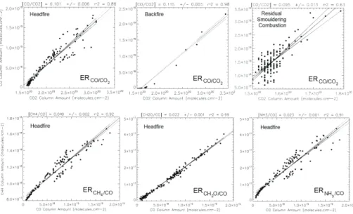
Molar emissions ratios were determined as described in Sect. 3.5.1. As an example, Fig. 6 shows a series of trace gas species column amounts plotted against those of CO2 and CO for examples of the three separate fire stages. The least squares lin-20

ear best-fits are shown in each case, with the gradient taken as the emissions ratio [ERX/CO₂ or ERX/CO] and the 95% confidence limits on the gradient providing an esti-mate of the emissions ratio uncertainty. Comparison of these ratios to those calculated via first converting the FTIR-determined column amounts to the equivalent excess mo-lar abundances (as per Sinha et al., 2003a) confirmed differences of less than 1%. 25

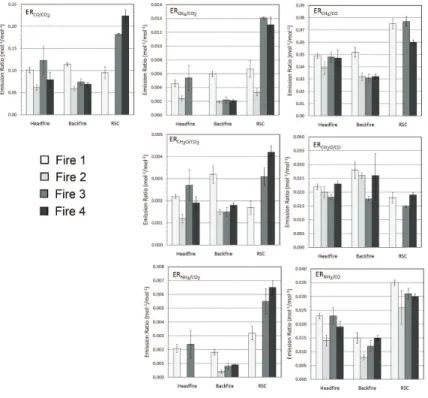
Emissions ratios of each targeted species to both CO2and CO were assessed in this way, and Table 3 details results for all fires, with a histogram of these data shown in Fig. 7 for easy intercomparison. As is commonly the case (Andreae and Merlet, 2001)

(20)

ACPD

11, 3529–3578, 2011

emission ratios

Title Page

Tables Figures

◭ ◮

Back Close

Full Screen / Esc

Discussion

P

a

per

|

Dis

cussion

P

a

per

|

Discussion

P

a

per

|

Discussio

n

P

a

per

|

for many gases there was usually a somewhat better correlation to CO than to CO₂ (expected due to their common preferential production during smouldering activity), but the ER_x/CO₂ ratio was nevertheless derived since it is required for later derivation of emissions factors (via Eqs. 5 and 6). Following Sinha et al. (2003a) we use the strength of the coefficient of determination (r2) between the abundance of a particular 5

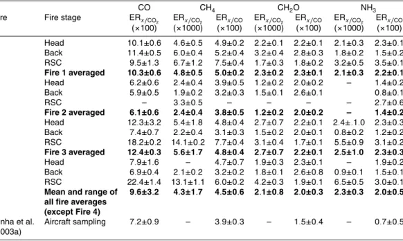
gas species and that of CO or CO2 to confirm the emissions ratio for that gas as well determined. Most had r2>0.7, and those species for which the coefficient of deter-mination fell below 0.4 are assumed to be poorly determined and are not shown. In particular the RSC Stage of Fire 2 generated low trace gas column amounts (three orders of magnitude lower than some other fires) from which meaningful ERs could not 10

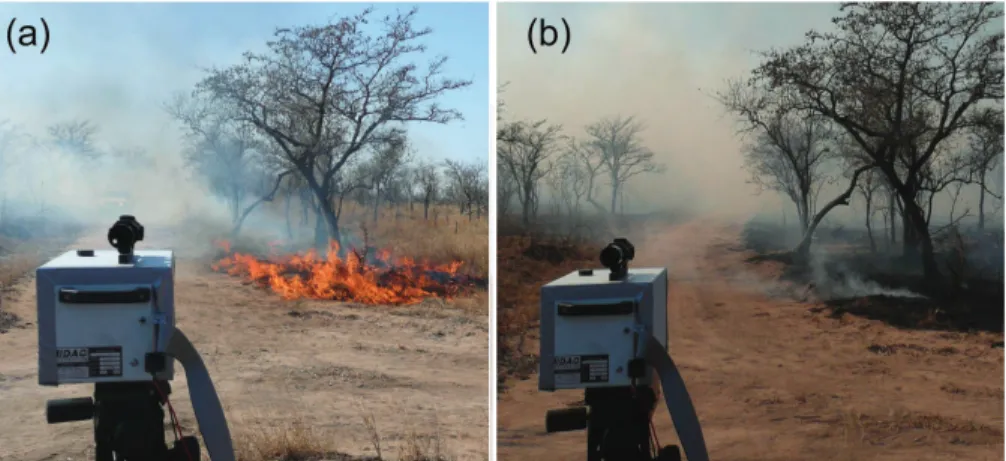
be calculated. This is confirmed by the photographs shown in Fig. 8, which demon-strate how Fire 2 failed to generate a significant “smoking zone” behind the advancing headfire. Lacaux et al. (1996) characterised a typical headfire plume as containing emissions from both the flaming front and a “smoking” zone located immediately be-hind, but since Fire 2 generated only a very weak smoking zone, emissions production 15

in the subsequent RSC stage would be expected to be similarly low.

Overall, our results confirm that in most cases emission ratios to CO₂(i.e., ER_x/_CO

2)

for CO, CH4 and NH3 are notably higher during the RSC stage as compared to the flaming stages, whereas those of CH2O are less so. Emission ratios to CO are also in general somewhat higher for CH₄ and NH₃ during the RSC stage than during the 20

flaming stages, but the reverse is true for CH2O. Results for Fire 1 appear to follow these trends less clearly than those of the other fires, for reasons discussed below. The contrasting relationships shown for formaldehyde are interpreted to result from its higher production during the pyrolysis phase, thus providing more limited opportunities for its creation during the RSC stage where flaming activity is absent (Koppmann et al., 25

2005).

(21)

ACPD

11, 3529–3578, 2011

emission ratios

Title Page

Tables Figures

◭ ◮

Back Close

Full Screen / Esc

Discussion

P

a

per

|

Dis

cussion

P

a

per

|

Discussion

P

a

per

|

Discussio

n

P

a

per

|

ERCO/CO₂ values determined for different savannah fires by Lacaux et al. (1996) var-ied over a (4.0–12.8)×10−2 range, rather similar to the (6.2–12.3)×10−2 range found

here. However, when Lacaux et al. (1996) weighted their separate ER measures for the headfire flaming and smoking zones by an estimate of the amounts of fuel be-lieved to have been consumed in each (an assumed ratio of 9:1, respectively) they 5

obtained lower ERCO/CO₂values (3.0-5.8)×10

−2

. The backfire ERCO/CO₂range of (3.4– 7.0)×10−2determined by Lacaux et al. (1996) is also lower than the (5.9–11.4)×10−2

range determined here. Lacaux et al. (1996) concluded that headfire and backfire ER_CO_/_CO

2 are quite comparable, a finding that our results generally confirm. Unlike

Cofer et al. (1996) who suggest ERCO/CO₂ of flaming and smouldering combustion for 10

KNP fires to be within a few percent of one another, our results suggest substantial dif-ferences can occur. Lacaux et al. (1996) determined smouldering stage ER_CO_/_CO

2 to

vary over a (12.1–20.8)×10−2range, similar to the (9.5–22.4)×10−2range found here

and certainly more different to the flaming stage ERCO/CO₂ than suggested by Cofer et al. (1996).

15

Our results for Fire 1 depart somewhat from those of the other fires, in particular in having a ERCO/CO₂ that is similar for all three fire stages (headfire, backfire and RSC). A possible cause maybe the large amount of (primarily elephant) dung present in the interior of the Fire 1 burn plot, which was not seen on any other plot and which contin-ued to burn for a long time after passage of the flaming front (Fig. 8c), thus contributing 20

substantially to smoking zone emissions in all three fire stages. Crockett and Engle (1999) show that burning of (North American Bison) dung ignited by grassfires can continue for very substantial periods after the flaming front has passed, and that the resultant combustion characteristics are very different to those of the underlying veg-etation fuel. Scholes et al. (1996) and Shea et al. (1996) both previously report dung 25

burning at some of the KNP burn plots, and though we did not measure EFs specifi-cally from burning dung, Keene et al. (2006) report that Southern African (cow) dung has an EF_CO around twice that of burning grasses, and an EF_CO

2 around half that of

(22)

ACPD

11, 3529–3578, 2011

emission ratios

Title Page

Tables Figures

◭ ◮

Back Close

Full Screen / Esc

Discussion

P

a

per

|

Dis

cussion

P

a

per

|

Discussion

P

a

per

|

Discussio

n

P

a

per

|

burning grass. Therefore, dung ERCO/CO₂ is close to four times that of grass, and this di_fference coupled with the extra fuel load provided by dung seems a possible cause of the similar ERCO/CO₂ measured across the three fire stages of Fire 1.

The fire averaged emissions ratios, calculated from the separate stage ERs weighted by the relevant FRE data, are also shown in Table 3. Even though the emissions ratio 5

characteristics of the RSC stage can be significantly different to those of the flaming stages, for all fires the vast majority of fuel consumption took place in the headfire and so the “fire averaged” ERs are dominated by the headfire contribution. This sug-gests that under conditions where FRE or other fuel consumption measurements are unavailable, including at unplanned wildfires, emissions ratio characterisation using 10

smoke emanating from the main fire front and neighbouring smoking zone is likely to be a relatively good representation of the “fire averaged” values, agreeing with the basic conclusions of Cofer et al. (1996).

Comparisons can be made between the ERs determined here and those from prior studies. It should be noted than many species transform as smoke ages, and thus the 15

measurement timing in relation to the causal fire should be carefully considered (Hobbs et al., 2003). Table 3 includes the relevant mean ER_x/_CO

2 values reported by Sinha et

al. (2003a) for non-aged fire smoke from similar KNP fires as studied here, but derived via gas chromatography and closed-path airborne FTIR spectroscopy. Comparison to the current results for CO, CH₄and CH₂O indicates overlap in the estimates derived via 20

the two approaches, despite the very different sampling and measurement approaches applied, further evidence for the validity of our extended open-path remote sensing approach. Our estimates of ER_NH

3/CO are, however, substantially greater than those

of Sinha et al. (2003a), and potential reasons for this are discussed in the following Section.

25

4.3 Emissions factors

(23)

ACPD

11, 3529–3578, 2011

emission ratios

Title Page

Tables Figures

◭ ◮

Back Close

Full Screen / Esc

Discussion

P

a

per

|

Dis

cussion

P

a

per

|

Discussion

P

a

per

|

Discussio

n

P

a

per

|

Uncertainties were calculated in quadrature from those associated with the trace gas ERs and the±10% uncertainty in the assumed fuel carbon content. Fire averaged EFs

for each species were again calculated by weighting the EFs calculated for each of the three fire stages by the relevant FRE measure. Table 4 also includes the EFs reported for Southern African savannah fires by Sinha et al. (2003a), which they calculated 5

from their measured ERs that are listed in Table 3. Also listed are EFs taken from the SAFARI-92 KNP airborne study of Cofer et al. (1996), EFs from the widely used database of Andreae and Merlet (2001) and updates, and from the SAFARI-92 and SAFARI-2000 campaigns (Ward et al., 1996; Keene et al., 2006, respectively). Our EFs for CO2are similar to those of all the past studies, and in particular are very close 10

to the values derived in the most recent study conducted in almost exactly the same KNP area (Sinha et al., 2003a). The same is true for CH4, but for CO our “fire averaged” mean EF is in general higher than the mean values determined in past works, though still within the range determined by Ward et al. (1996) and Keene et al. (2006).

In contrast to the relatively good agreement between our EFs and those presented 15

by Andreae and Merlet (2001) for the dominant carbonaceous species, we find the EF of formaldehyde to be significantly elevated (by a factor of∼4–8), though their more

recent update included in Table 4 lowers the difference somewhat. Our results there-fore confirm the findings of Sinha et al. (2003a) and Yokelson et al. (2003) of significant departures from literature values of savannah fire EF_CH

2O, a species directly involved

20

in the production of tropospheric ozone. However, unlike these prior works we do not find major differences between KNP NH3 emission factors and those presented by Andreae and Merlet (2001) and its updates, and indeed our results are closer to the values quoted in Andreae and Merlet than to those of Sinha et al. (2003a). We note that without appropriate subtraction of the ambient emission signal (which Fig. 3 25

confirms is highly significant at the lower wavenumbers used to retrieve ammonia) our NH3 column amounts and thus EFs would be underestimated by ∼60%. Thus we were careful to utilize the approach of M ¨uller et al. (1999) when retrieving NH3column amounts, and rather than ambient background influences the cause of the discrepancy

(24)

ACPD

11, 3529–3578, 2011

emission ratios

Title Page

Tables Figures

◭ ◮

Back Close

Full Screen / Esc

Discussion

P

a

per

|

Dis

cussion

P

a

per

|

Discussion

P

a

per

|

Discussio

n

P

a

per

|

in EF_NH

3 maybe the contrasting measurement methodologies used here and by Sinha

et al. (2003a) and Yokelson et al. (2003). In particular, Yokelson et al. (2003) identified NH3 to be the only targeted species whose concentration was noticeably affected by the brief residence time spent in the closed cell used to contain the sample. It was suggested that mean EFNH₃ underestimations of 5–20% may result, though underes-5

timations of up to 50% were apparently seen in pre-flight laboratory tests (Yokelson et al., 2003). Our open path method does not suffer from this effect, potentially ex-plaining at least some of the noted difference in EFNH₃. A further contributory factor may come from the work of Keene et al. (2006), who found fuel-specific EFNH₃ to differ substantially between the different KNP fuel components, most probably due to diff er-10

ing nitrogen contents. This makes each EF_NH

3 highly dependent upon the mix of fuels

consumed, and suggests potentially high variability across space and time.

4.4 MCE and fire pixel brightness temperature

Since flaming combustion occurs at a higher temperature than smouldering combus-tion (Lobart and Warnatz, 1993) it has been suggested that fire temperature estimates 15

derived from airborne or spaceborne Earth observation maybe useful in broadly clas-sifying combustion into predominately flaming (i.e., higher MCE) or smouldering (i.e., lower MCE) activity (e.g., Dennision et al., 2006; Zhukov et al., 2006). Since ERs and EFs can clearly vary substantially between these phases, such discrimination may in future be able to enhance emissions estimation procedures. Since both plume MCE 20

and fire pixel brightness temperature (BT) data are available for the headfire and RSC Stages of Fires 1 and 3 we have some opportunity to examine this potential. Our con-clusions must be limited however, since without multi-spectral airborne IR data we can examine pixel-integrated BTs only, which are lower than the fires true radiative tem-perature due to the area of combustion commonly underfilling the imager pixels. This 25

(25)

ACPD

11, 3529–3578, 2011

emission ratios

Title Page

Tables Figures

◭ ◮

Back Close

Full Screen / Esc

Discussion

P

a

per

|

Dis

cussion

P

a

per

|

Discussion

P

a

per

|

Discussio

n

P

a

per

|

and other fire processes, but nevertheless the final two panels of Fig. 5 do demonstrate that the Fire 1 MCE and BT data do show a degree of temporal similarity. MCE starts at almost 1.0 during the backfire, decreases into the headfire (mean±σof 0.86±0.06),

and falls further during the period of RSC towards the end of the burn (0.76±0.07),

indicating a transition from flaming-dominated to completely smouldering combustion. 5

Maximum BT also decreases over the same time interval (headfire 723±66 K vs. RSC

595±47 K) as does, albeit less significantly, mean BT (headfire 541±21 K vs. RSC

512±10 K). Data from Fire 3 confirms this pattern of decreasing MCE and BT as the

combustion moves from flaming to increased smouldering, albeit both the MCE and BT values of the different stages are closer than was seen at Fire 1 (MCE: headfire 10

0.89±0.05 vs. RSC 0.85±0.01; max BT: headfire 595±62 K vs. RSC 555±41 K; mean

BT: headfire 520±17 vs. RSC 512±18 K).

5 Summary and conclusions

A unique high temporal resolution trace gas and FRP dataset has been collected for a series of multi-hectare fires conducted in Kruger National Park, South Africa us-15

ing extended OP-FTIR spectroscopy operated over 150–250 m pathlengths. These measurements were supplemented by airborne optical and thermal imaging. Follow-ing an early demonstration by Griffith et al. (1991), extended OP-FTIR spectroscopy has been relatively little exploited for vegetation fire plume analysis, but reductions in size and cost, and increases in the performance and availability of Stirling-cooled 20

detector systems, have made such deployments increasingly practicable. Our OP-FTIR setup allowed multiple smoke chemical constituents to be probed simultaneously and at a very high temporal resolution across a large proportion (or even the totality) of the advected plume cross section, avoiding many limitations of point-sampling ap-proaches. Trace gas column amounts were derived from the single beam IR spectra 25

using a spectral forward model coupled to a non-linear least squares fitting approach, avoiding the need for experimentally determined reference spectra. The method is

(26)

ACPD

11, 3529–3578, 2011

emission ratios

Title Page

Tables Figures

◭ ◮

Back Close

Full Screen / Esc

Discussion

P

a

per

|

Dis

cussion

P

a

per

|

Discussion

P

a

per

|

Discussio

n

P

a

per

|

sufficiently sensitive to detect path-averaged CO mixing ratio variations of around 10 ppbv (0.001 µmol mol−1) across the 150–250 m optical paths used here. The re-trieved trace gas column amounts allow for the calculation of emissions ratios (ERs) and emissions factors (EFs) for each stage of the studied fires, and stage-specific fire radiative energy (FRE) measures calculated from airborne IR imagery allowed for the 5

determination of “fire averaged” ERs and EFs using a “weighted-mean” approach. The FRE data indicate that only a few percent of total fuel consumption actually occurs in the RSC stage, so even though ERs and EFs are substantially higher for many com-pounds in the RSC stage, sampling of headfire activity alone actually maybe sufficient for the general assessment of “fire averaged” ERs and EFs in the field, at least in this 10

savannah environment. There therefore appears to be only a limited requirement for concurrent airborne thermal imager observations in campaigns targeting the determi-nation of emissions ratios and emissions factors using OP-FTIR methods, at least in environments with relatively insignificant amounts of burning of organic litter and soil layers.

15

We focused on a set of key compounds related preferentially to the pyrolysis (CH2O), flaming (CO₂) and smoldering (CO, CH₄, NH₃) combustion phases. We find ERs for headfires and backfires to be similar, and generally rather different that those seen in the residual smouldering combustion (RSC) stage, apart from at one fire where burning elephant dung appears to have contributed substantially to the emissions characteris-20

tics. With CO2 as the reference species, ERs from the residual smouldering com-bustion stage are otherwise notably higher than for the flaming stages. Apart from for ammonia, our mean fire averaged ERs lie relatively close to those calculated previously by Sinha et al. (2003a) via airborne sampling in the same study area, though are gen-erally a little higher (by up to 33%; see last rows of Table 3). CO2and CH4 emissions 25

factors derived from the relevant emission ratios show good agreement with those of other studies, including Andreae and Merlet (2001) and subsequent updates. Our EF for carbon monoxide is, however, somewhat higher (by ∼45–85%) than the average