www.atmos-chem-phys.net/10/565/2010/ © Author(s) 2010. This work is distributed under the Creative Commons Attribution 3.0 License.
Chemistry
and Physics
Trace gas and particle emissions from domestic and industrial
biofuel use and garbage burning in central Mexico
T. J. Christian1, R. J. Yokelson1, B. C´ardenas2, L. T. Molina3,4, G. Engling5, and S.-C. Hsu5
1University of Montana, Department of Chemistry, Missoula, MT, USA
2National Center for Environmental Research and Training, National Institute of Ecology/SEMARNAT, Mexico, DF, Mexico 3Department of Earth, Atmospheric and Planetary Science, Massachusetts Institute of Technology, Cambridge, MA, USA 4Molina Center for Energy and Environment, La Jolla, CA, USA
5Research Center for Environmental Changes, Academia Sinica, Taipei, Taiwan, ROC, Taiwan Received: 1 April 2009 – Published in Atmos. Chem. Phys. Discuss.: 21 April 2009
Revised: 23 December 2009 – Accepted: 23 December 2009 – Published: 21 January 2010
Abstract. In central Mexico during the spring of 2007 we measured the initial emissions of 12 gases and the aerosol speciation for elemental and organic carbon (EC, OC), anhy-drosugars, Cl−, NO−
3, and 20 metals from 10 cooking fires, four garbage fires, three brick making kilns, three charcoal making kilns, and two crop residue fires. Global biofuel use has been estimated at over 2600 Tg/y. With several simple case studies we show that cooking fires can be a major, or the major, source of several gases and fine particles in devel-oping countries. Insulated cook stoves with chimneys were earlier shown to reduce indoor air pollution and the fuel use per cooking task. We confirm that they also reduce the emis-sions of VOC pollutants per mass of fuel burned by about half. We did not detect HCN emissions from cooking fires in Mexico or Africa. Thus, if regional source attribution is based on HCN emissions typical for other types of biomass burning (BB), then biofuel use and total BB will be under-estimated in much of the developing world. This is also sig-nificant because cooking fires are not detected from space. We estimate that∼2000 Tg/y of garbage are generated glob-ally and about half may be burned, making this a commonly overlooked major global source of emissions. We estimate a fine particle emission factor (EFPM2.5) for garbage burning
of∼10.5±8.8 g/kg, which is in reasonable agreement with very limited previous work. We observe large HCl emission factors in the range 2–10 g/kg. Consideration of the Cl con-tent of the global waste stream suggests that garbage burning
Correspondence to:R. J. Yokelson
(bob.yokelson@umontana.edu)
1 Introduction
In developed countries most of the urban combustion emis-sions are due to burning fossil fuels. Fossil fuel emisemis-sions are also a major fraction of the air pollution in the urban areas of developing countries. However, in the developing world, the urban areas are embedded within a region that fea-tures numerous, small-scale, loosely regulated combustion sources due to domestic and industrial use of biomass fuel (biofuel) and the burning of garbage and crop residues. The detailed chemistry of the emissions from these sources has not been available and the degree to which these emissions affect air chemistry in urban regions of the developing world has been difficult to assess. As an example, we note that Raga et al. (2001) reviewed 40 years of air quality measurements in Mexico City (MC) and concluded that more work was needed on source characterization of non fossil-fuel com-bustion sources before more effective air pollution mitigation strategies could be implemented. The 2003 MCMA (Mexico City Metropolitan Area) campaign (Molina et al., 2007) and the 2006 MILAGRO (Megacity Initiative: Local and Global Research Observations) campaign. Molina et al. (2008) fo-cused on fixed-point monitoring of the complex MCMA mix of pollutants at heavily instrumented ground stations and on airborne studies of the outflow from the MCMA region. Ex-plicit source characterization for biomass fires in the MCMA region was part of MILAGRO 2006, but only for landscape-scale open burning (e.g. forest fires in the mountains adjacent to MCMA, Yokelson et al., 2007).
Our 2007 ground-based MILAGRO campaign employed an approach that was complementary to most of the earlier work. With a highly mobile suite of instruments, we ac-tively located representative sources of biofuel and garbage burning on the periphery of the MCMA and throughout cen-tral Mexico and measured the initial trace gas and particle emissions directly within the visible effluent plumes of these sources. The results should help interpret the data from both the fixed monitoring stations in the MCMA (e.g.T0,T1,T2, etc.) and from aircraft in the outflow, (Molina et al., 2008). Our source characterization also has global significance due to the widespread occurrence of these sources throughout the developing world as summarized next.
Recent global estimates of annual biofuel consumption in-clude 2897 Tg dry matter (dm)/y (Andreae and Merlet, 2001) and 2457 Tg dm/y (Fernandes et al., 2007), making it the second largest type of global biomass burning after savanna fires. An estimated 80% of the biofuel is consumed for do-mestic cooking, heating, and lighting mostly in open cook-ing fires burncook-ing wood, agricultural waste, charcoal, or dung within homes (Dherani et al., 2008). The balance of the bio-fuel is consumed mostly by low-technology, largely unreg-ulated, micro-enterprises such as brick or tile making kilns, restaurants, tanneries, etc. While individual “informal firms” are small, their total number is very large, e.g.∼20 000 brick making kilns in Mexico (Blackman and Bannister, 1998).
Thus, this “informal sector” of the economy accounts for over 50% of non-agricultural employment and 25–75% of gross domestic product in both Latin America and Africa (Ranis and Stewart, 1994; Schneider and Enste, 2000). Bio-fuel use is thought to occur mainly in peri-urban and rural areas where biofuel is readily available although use of trans-ported charcoal is known to occur in cities (Bertschi et al., 2003). The quantification of biofuel use has been based on surveys of the rural population and there are not good esti-mates of how much may occur in urban areas.
McCulloch et al. (1999) calculated the 1990 garbage pro-duction from the 4.5 billion people included in the Reactive Chlorine Emissions Inventory as 1500 Tg. Scaling to the cur-rent global population of 6 billion suggests that 2000 Tg is an approximate, present global value. If half of this garbage is burned in open fires or incinerators (McCulloch et al., 1999) and it is 50% C, it would add 500 Tg of C to the atmosphere annually. This is about 7% of the C added by all fossil fuel burning (Forster et al., 2007). This crude estimate is fairly consistent with data from the remote Pacific in which 11±7% of the total identified organic mass in the ambient aerosol was phthalates, ostensibly from garbage burning (Table 6, Simoneit et al., 2004b). It is most economical to burn urban-generated garbage in, or near, the major population centers that produce it. In addition, an estimated 12–40% of house-holds in rural areas of the US burn trash in their backyards, (USEPA, 2006). Thus, most garbage burning occurs in close proximity to people, despite estimates that garbage burning is the major global source of some especially hazardous air toxics such as dioxins (Costner, 2005, 2006).
The burning of crop residue in fields is generally consid-ered to be the fourth largest type of global biomass burning with estimates including 540 Tg dm/y (Andreae and Merlet, 2001) and 475 Tg dm/y (Bond et al., 2004). Because cities are often located in prime agricultural regions, they may ex-pand into areas where crop residue burning is a major activity and is sometimes the dominant local source of air pollution, (Canc¸ado et al., 2006).
In this study we measured the initial emissions of 12 of the most abundant gases, and the aerosol speciation for el-emental and organic carbon (EC, OC), anhydrosugars, Cl−, NO−3, and 20 metals from domestic and industrial biofuel use, garbage burning, and crop residue fires. In the follow-ing sections the measurements are described in detail and the implications of selected results are discussed.
2 Experimental details
2.1 Source types and site descriptions
Table 1.Sampling source types and locations.
Type Location Date (2007) Lat Lon
Open cook San Pedro Benito Ju´arez, Atlixco, Puebla 18 Apr 18.95 −98.55
Open cook San Pedro Benito Ju´arez, Atlixco, Puebla 19 Apr 18.95 −98.55
Open cook San Juan Tumbio, Michoac´an 8 May 19.50 −101.77
Open cook San Juan Tumbio, Michoac´an 8 May 19.50 −101.77
Open cook Comachu´en, Michoac´an 9 May 19.57 −101.90
Open cook Comachu´en, Michoac´an 9 May 19.57 −101.90
Open cook Comachu´en, Michoac´an 9 May 19.57 −101.90
Open cook GIRA lab, Tzentzenguaro, Michoac´an 10 May 19.53 −101.64
Patsari cook GIRA lab, Tzentzenguaro, Michoac´an 10 May 19.53 −101.64
Patsari cook Rancho de ´Alvarez, Michoac´an 11 May 19.54 −101.51
Charcoal kiln San Gaspar de lo Bendito, Atlixco, Puebla 17 Apr 19.00 −98.54
Charcoal kilna Hueyitlapichco, Atlixco, Puebla 19 Apr 18.97 −98.56
Charcoal kilna Hueyitlapichco, Atlixco, Puebla 20 Apr 18.97 −98.56
Brick making kiln Teoloyucan, Edo. M´exico 24 Apr 19.77 −99.19
Brick making kiln Barrio M´exico 86, Edo. M´exico 27 Apr 19.41 −98.91
Brick making kiln Silao, Guanajuato 2 May 20.94 −101.42
Landfill Soyaniquilpan, Edo. M´exico 23 Apr 20.01 −99.49
Landfill Coyotepec, Edo. M´exico 24 Apr 19.81 −99.22
Landfill Tolcayuca, Hidalgo 25 Apr 19.97 −98.92
Landfill San Mart´ın de las Pir´amides, Edo. Mex. 26 Apr 19.70 −98.80
Barley stubble Rancho de Don Ignacio, Guanajuato 30 Apr 20.60 −101.22
Barley stubble Rancho de Don Ignacio, Guanajuato 1 May 20.60 −101.22
aTwo separate kilns at one location.
source types listed in Table 1 and shown in a map available as supplementary material (http://www.atmos-chem-phys. net/10/565/2010/acp-10-565-2010-supplement.pdf). The sources include eight indoor open wood cooking fires, two indoor wood cooking fires in Patsari stoves, three charcoal making kilns (from two sites), three brick making kilns, four garbage burns in peri-urban landfills, and two barley stubble field burns.
All but one of the open wood cooking fire measurements were conducted in rural and semi-rural homes during actual cooking episodes. The cooking fire in the laboratory of the Interdisciplinary Group on Appropriate Rural Technology (GIRA) was a simulation using an authentic open cook stove and typical fuel wood. For six of the eight homes in which we sampled, the kitchen was housed in a separate building. For the other two, the kitchen was part of the main dwelling with a wall separating it from the sleeping area. Ventilation in all cases was by passive draft through door and window openings, cracks in the walls between boards, and horizontal openings where roof meets wall. Six of the eight kitchens had a dirt floor, seven were constructed of wood and one of brick. A variety of biofuels were available to the home-owners, including wood, corn cobs, corn stalks, and char-coal. The primary fuel in all these homes, and the fuel used in all the fires we measured, was oak or pine collected lo-cally by hand. Cooking fires were built either directly on the
ground within a ring of three rocks, or on a mud and mor-tar, u-shaped, raised open stove. In one instance the “stove” was a dirt-filled metal bucket with rocks on top. In the homes that we visited a typical food preparation regimen began with a small, hot, flaming fire to quickly boil a pot of water, which is then loaded with beans and set off to the side to simmer. As the fire begins to die back, the cook begins making tor-tillas. Wood is fed gradually to the fire to maintain the right amount of heat and when the cooking ends the fire is gener-ally snuffed out to conserve fuel. A cooking session might last several hours depending on how much food is needed in the next few days. The sample lines of all the instruments were co-located at ∼1 m above the fire over the course of the cooking operation. The cook and her youngest children typically remain inside the kitchen for as long as it takes to prepare the food.
largest single cause of mortality globally in children under five (Smith et al., 2004; Dherani et al., 2008). It is also of interest that reactions on the chimney surface could modify the emissions (Christian et al., 2007). The chimney does not eliminate all the indoor pollutants because the fire box has an open front that can leak emissions into the room. Also, the chimney emissions may at times be recirculated into the kitchen from outdoors. We sequentially measured first the kitchen air above the stove, and then the chimney emissions from two different Patsari stoves in P´atzcuaro. One was lo-cated in a rural kitchen and the other was a newer model located in the GIRA lab’s simulated kitchen.
We sampled three charcoal making kilns in a forested area between MC and Puebla. An excavation∼5 m in diameter is dug by hand and kindling (dry needles, leaves, and twigs) is laid down. Oak logs are stacked in the center and a network of interlaced green oak branches is placed over the top. The excavated dirt is then packed on top to complete the earthen kiln, which has about a dozen vents around the circumfer-ence. A kiln of this design yields 200–250 kg of charcoal in about eight days. The supporting oak branches burn away slowly and the kiln must be rebuilt once or more during its lifetime to prevent it from collapsing and smothering the fire. The two kilns at the Hueyitlapichco site were constructed on consecutive days. We sampled them on their second and third day of operation on 19 April, and on their third and fourth day of operation on 20 April. At the San Gaspar site we sampled a single kiln on its fifth day of operation.
Brick making kilns in central Mexico are constructed from bricks. The fire bed and base walls are permanent and often built at the bottom of an excavation, which provides some in-sulation for the fire bed. There are several large, permanent mortar or concrete “crossbeams” above the fire bed. Green bricks are stacked to a height of several meters on the cross-beams (spaced to allow even heat circulation). Brick walls and a roof are then built up around the whole assembly. A fire is lit and fuel is shoveled or thrown in until the desired temperature is reached. Fuel is then added, as needed, to maintain that temperature around the clock for 1–2 days. At varying times each kiln operator uses mortar to seal the walls and most of the roof. Some owners allow the kiln to venti-late freely through the walls and roof for a day before sealing with mortar, claiming this gives a more uniform bake. Others seal the walls and roof before ignition. Kilns number 1 and 2 were burning fuel that was mostly wood waste products that had been hauled onto the site by dump truck. About 90% of this fuel was sawdust by volume. The remainder was di-vided fairly evenly between wood scraps, plywood, and par-ticle board. A small fraction (less than 1%) was paper and cardboard. Brick kiln number 3 was using only scrap lum-ber while we made measurements. We were unable to visit a fourth kiln near Silao that was reportedly burning used motor oil for fuel and a fifth kiln near Salamanca that was burning domestic waste scavenged from a nearby landfill. The raw material for bricks is soil carved by hand from the ground
in the vicinity of the kiln. The soil is mixed with water and manure or other organic waste and stomped barefoot to form a thick paste. The paste is then pressed into a mold and over-turned one by one into rows to dry in the sun. Once they are dry enough to handle, the green bricks are stacked (in the shade if possible) and covered to prevent too rapid drying and cracking. Two of the brick kilns were sized to fire 10– 12 000 bricks at a time; the third (brick kiln 2) was about three times larger. Kilns of this design are typical for Latin America and Africa, while more efficient designs – and coal fuel – are more common in Asia.
All four garbage burning fires were in the municipal land-fills of peri-urban communities north of Mexico City. Only one landfill (Coyotepec, garbage fire 2) was burning when we arrived. At the other three sites we ignited relatively small, representative sections of refuse under the direction of local authorities. The landfills held typical household and light in-dustrial refuse. Plastic was by far the most abundant material present. The following list is an approximate accounting of the composition of the waste stream for these landfills, in roughly diminishing order:
– plastic: bottles, bags, buckets, containers, toys, wrap-pers, Styrofoam
– paper: newspaper, magazines, cardboard boxes, food containers
– organic: fruit, vegetables (food waste)
– textile/synthetic fiber: cotton/nylon clothing, scraps
– rubber/leather: neoprene (in one case), sandals, shoes, scraps
– glass: bottles, jars
– vegetation: garden waste, brush, grass
– metal: soup cans, buckets, oil filters, aluminum foil
– ceramic: cups, dishes, cookware
– other waste materials
0.0 0.4 0.8 1.2 1.6
0 20 40 60 80 100
ΔCO ppm
Δ
CΗ
3
Ο
Η
ppm
NLLS SS Linear (all)
ER (slope) = 0.014 r2 = 0.98
Fig. 1.An example of the determination of the fire-integrated emis-sion ratio for an open wood cooking fire by plotting the excess mix-ing ratios of methanol versus those of CO. The excess methanol is shown as determined by both nonlinear least squares synthetic cali-bration (NLLS) and spectral subtraction (SS).
The agricultural waste burns took place in two adja-cent, ∼2 ha barley fields northwest of Salamanca. The fields had been mechanically harvested so all that re-mained were standing stalks (stubble, ∼15 cm) and a mat of broken stalks and chaff, all of it tinder dry. Photographs of many of the field sites described above can be found at http://www.cas.umt.edu/chemistry/faculty/ yokelson/galleries/album Mex/index.html.
2.2 Instrumentation
The primary instrument for measuring trace gas emissions was our mobile, rolling cart-based Fourier transform in-frared spectrometer (Fig. 2, Christian et al., 2007). It is rugged, easily transported, optionally self-powered, and can be wheeled to remote sampling sites. The optical bench is isolated from the chassis with wire rope shock absorbers (Aeroflex) and holds a MIDAC 2500 spectrometer, White cell (Infrared Analysis, path length 9 m), MCT detector (Graseby), and transfer and focusing optics (Janos Technol-ogy). Continuous temperature (Minco) and pressure (MKS) sensors are mounted inside the cell. Other onboard fea-tures include a laptop computer, A/D and AC/DC convert-ers, and a 73 amp hour 12 V battery. Sample air is drawn into the cell by an onboard DC pump through several me-ters of 0.635 m o.d. corrugated Teflon tubing. Each sam-ple was held in the cell for one minute using manual Teflon valves while IR spectra were co-added to increase the signal to noise ratio. We used nonlinear least squares, synthetic cal-ibration (Griffith, 2002) to retrieve excess mixing ratios from the spectra for water (H2O), carbon dioxide (CO2), carbon monoxide (CO), methanol (CH3OH), methane (CH4), ethy-lene (C2H4), propyethy-lene (C3H6), acetyethy-lene (C2H2), formalde-hyde (HCHO), and hydrogen chloride (HCl). We used spec-tral subtraction (Yokelson et al., 1997) to retrieve excess
mix-y = -79.699x + 79.063
R2
= 0.53
0 2 4 6 8 10 12
0.90 0.91 0.92 0.93 0.94 0.95 0.96 0.97 0.98
MCE
EF
C
H4
(g
/k
g
)
Current Study Andreae and Merlet (2001) Johnson et al (2008) Zhang et al (2000) Bertschi et al (2003) Brocard et al (1998) Linear (All)
Fig. 2.Variation of the methane emission factor with MCE for open wood cooking fires.
ing ratios for CH3OH, C2H4, C3H6, C2H2, ammonia (NH3), formic acid (HCOOH, also denoted HFo), and acetic acid (CH3COOH, also HAc). At a path length of 9 m the detec-tion limit for most gases was∼50–200 ppb while typical an-alyte mixing ratios were in the thousands of ppb or larger. The above gases accounted for all the quantifiable features in the IR spectra. The typical uncertainty for mixing ratios was±10% (1σ). For CO2, CO, and CH4, the uncertainties were 3–5%. More complete descriptions of the system and spectral analyses are given in Christian et al. (2007).
After the campaign we checked for changes in analyte concentrations that might occur during the one-minute stor-age period in the FTIR cell due to adsorption or other rea-sons (Yokelson et al., 2003). The average NH3concentration in the cell during one minute of signal averaging (the typical sampling time used in Mexico) was about 71% of its initial level. The average HCl was∼93% of its initial level for the same interval. The ammonia and HCl results reported here have been adjusted upward to account for these cell losses.
ions were determined with ion chromatography (Hsu et al., 2008b). In brief, a Dionex DX120 ion chromatograph was equipped with a conductivity detector and AS4A and CS12A columns for anion and cation separation, respectively. The eluents used for the respective ion separations were 1.7 mM NaHCO3and 1.8 mM Na2CO3at a flow rate of 1.5 mL/min for anions and 20 mM CH4O3S for cations at a flow rate of 1.0 mL/min. We analyzed the quartz filters for trace elements using inductively coupled plasma-mass spectrometry (ICP-MS) (Hsu et al., 2008a, 2010).
We did not sample particles with Teflon filters, which are used for gravimetric determination of total PM2.5.
How-ever, we did deploy an integrating nephelometer (Radiance Research M903) that measured particle light-scattering at 530 nm and 1 Hz. The nephelometer was calibrated with par-ticle free zero air and CO2 before and after the campaign. The M903 nephelometer response was attenuated at the high-est concentrations we encountered in Mexico. Thus, we ap-plied a correction factor to those high values based on direct comparison in laboratory smoke between the M903 and a TSI 3563 nephelometer, which does have a sufficiently large linear range. The M903 nephelometer output (bscat, m−1) has been compared directly to gravimetric PM2.5 determina-tions on cooking fires in both Honduras (Roden et al., 2006) and Mexico (Brauer et al., 1996). For dry, fine particles the conversion factor depends mostly on the EC/OC ratio of the particles. Our average EC/OC ratio (0.284) for cooking fires was very close to that reported by Roden et al. (2006) for their cooking fires (0.267). Thus, we used the average of the two conversion factors from the other cooking fire studies to convert light-scattering data from our cooking fires to an estimated total PM2.5as follows:
bscat(530nm,273K,1atm)×552000±75000 (1)
=PM2.5(µg/m3,273K,1atm)
(The conversion factor is equivalent to a mass scattering effi-ciency of 1.8). This approach probably gives an uncertainty in our average PM2.5for cooking fires of about 20–40%.
The light scattering by the particles from the other com-bustion types could be very different so we did not estimate a total PM2.5for these sources from the nephelometer data. However, we do report the mass sum of the particle con-stituents on the quartz filters. In this sum, we multiply the OC by a conservative factor of 1.4 to account for non-carbon organic mass (Aiken et al., 2008). The species measured include most of the major particulate components with the exception of sulfate and ammonium, which accounted for only a few percent of particle mass in other Mexican biomass burning particles (Yokelson et al., 2009). Thus, the sum of detected species is likely not more than 10–30% lower than the total PM2.5.
We also deployed a CO2instrument (LICOR LI-7000) that was calibrated both before and after the campaign (negligi-ble drift) with NIST-tracea(negligi-ble standards spanning the CO2
range encountered in the field. The CO2, nephelometer, and filter sampling systems shared a single inlet (conductive sil-icon tubing) that was often co-located with the FTIR sample line. In the cases where the FTIR mobility allowed sampling of the emissions at more points than the other instruments, the accurate determination of CO2by both the LICOR and the FTIR allowed coupling the two data sets. CO2was also used to correlate the particle measurements to the trace gases measured by FTIR as described in detail elsewhere (Yokel-son et al., 2009; Yokel(Yokel-son et al., 2007).
2.3 Calculation of emission ratios and emission factors
An emission ratio (ER) is defined as the initial molar excess mixing ratio (EMR) of one species divided by that of an-other species, most commonly CO or CO2. EMR is simply the molar amount of a species above the background level and is designated with the Greek capital delta – e.g.1CO,
1CH4,1X, etc. Modified combustion efficiency (MCE) is defined as the ratio1CO2/(1CO2+1CO) and is useful for estimating the relative amounts of flaming and smoldering combustion during a fire, with high MCE corresponding to more flaming (Ward and Radke, 1993). To estimate the fire-average ER for a species “X” we plot1X for all the sam-ples of the fire versus the simultaneously measured1CO (or
1CO2) and fit a least squares line with the intercept forced to zero. The slope is taken as the best estimate of the ER as explained in more detail in Yokelson et al. (1999). Figure 1 is an example of this type of plot showing the CH3OH/CO ER derived from 10 FTIR samples obtained over the course of a wood cooking fire.
An emission factor for any species “X” (EFX) is the mass of species X emitted per unit mass of dry fuel burned (g com-pound per kg dry fuel). EF can be derived from a set of molar ER to CO2using the carbon mass balance method, which as-sumes that all of the burned carbon is volatilized and that all of the major carbon-containing species have been mea-sured. It is also necessary to measure or estimate the carbon content of the fuel. For the fires using biomass fuel we as-sumed a dry, ash-free carbon content of 50% by mass (Susott et al., 1996). For the garbage fires, which contained only some biomass, we estimated the relative abundance of the materials present from photographs. We then calculated the overall carbon fraction based on those proportions and car-bon content estimates for each type of material (IPCC, 2006; USEPA, 2007). Table 2 shows that this procedure resulted in an overall carbon fraction of 40% for the landfill materi-als. The EF calculations for a charcoal kiln are complex be-cause the fuel carbon fraction increases with time. We used a procedure identical to that described in detail by Bertschi et al. (2003).
EFPM2.5 for the cooking fires were calculated by multiplying the fire-integrated PM2.5 to CO2 mass ra-tio (gPM2.5/gCO2 as measured by the nephelometer and
Table 2.Estimate of the carbon content of Mexican peri-urban land-fills.
Category Relative proportion Estimated Carbon by volumea mass fractionb fractionc
plastic 0.65 0.30 0.74
paper 0.10 0.15 0.46
organic (food waste) 0.05 0.05 0.38 textile/synthetic fiber 0.05 0.05 0.60
rubber/leather 0.05 0.05 0.76
glass 0.02 0.05
vegetation 0.01 0.05 0.50
metal 0.01 0.05
ceramic 0.01 0.05
other 0.05 0.20
net 1.00 1.00 40%
aVisual estimate of relative volumes of the most prominent waste
materials from four Mexican landfills. b Rough estimate of rel-ative mass for each material type. c Combined estimates from IPCC (2006) Table 2.4 and USEPA (2007) Annex 3 Tables A-125 to A-130.
FTIR). A similar method was applied to individual particle species based on net mass loading of fire-integrated filters, volumetric flow, and EFCO2.
3 Results and discussion
3.1 Cooking fires
Trace gas ER and EF and particle EF based on light scat-tering for our cooking fires are given in Table 3. The first 10 columns of data are the eight open wood cooking fires plus a column each for the average and standard deviation. The next three columns are the EF and average for the two Patsari stoves as sampled in the kitchen. The last three columns are the analogous data from the outdoor chimney exhaust of the same two Patsari stoves. The EF for individ-ual particle species measured on the quartz filters are given for all the fires in Table 4. Open wood cooking fires are the main global type of biofuel use and we get an idea of the global variability in this source by comparing EF from selected studies for some of the more commonly measured emissions (CO2, CO, CH4, and PM).
Figure 2 shows EFCH4 versus MCE (a function of CO and CO2) for those studies, including this one, where CO, CO2, and CH4 data were all available. A range of MCE from about 0.90 to 0.98 (avg 0.946) occurs naturally for in-dividual fires in these studies. This leads to about a factor of 10 variation in EFCH4for individual fires, but the study-average values agree reasonably well with each other. Some notes about the studies included in Fig. 2 follow. The John-son et al. (2008) study was conducted in the same villages in Michoac´an where the majority of our cooking fires were sampled. The authors sampled eight open cooking fires and
y = -15.168x + 20.286 R2
= 0.0403
0 2 4 6 8 10 12 14 16 18 20
0.86 0.88 0.90 0.92 0.94 0.96 0.98
MCE
E
FPM
(
g
/k
g
)
Current Study
Andreae and Merlet (2001)
Johnson et al (2008)
Zhang et al (2000)
Roden et al (2009)
Roden et al (2006)
Linear (All)
Fig. 3.Variation of the particle emission factor with MCE for open wood cooking fires. (This work and Andreae and Merlet 2001 – PM2.5, Roden et al. (2006) – PM4, all others TPM).
13 Patsari stoves and reported fire-integrated trace gas emis-sion factors based on gas chromatographic analysis of smoke collected in Tedlar bags over the course of each fire. Zhang et al. (2000) set up a simulated kitchen in China and, us-ing similar samplus-ing methods as Johnson et al., reported fire-integrated emissions from a few open stove types with var-ious common fuels. The Zhang et al. (2000) data in Fig. 2 include only their wood and brush fuel types. Bertschi et al. (2003) reported the average EF for 3 open wood cook-ing fires in a village in Zambia. Brocard et al. (1996) re-ported the average EF for 43 open wood cooking fires on the Ivory Coast. The Andreae and Merlet (2001) data point is a widely-used global estimate derived from the literature. The Bertschi et al. (2003) EFCH4 appears higher than the trend and the Brocard et al. (1996) EFCH4 lower, but these data are consistent with a tendency toward greater variability as the relative amount of smoldering emissions increases in biomass burning fires (Christian et al., 2007; Yokelson et al., 2008).
Table 3. Normalized emission ratios (ER, mol/mol) and emission factors (EF, g/kg dry fuel) for 8 open wood cooking fires and 2 Patsari stoves in central Mexico.
Open cooka Open cook Patsarib Patsari chimneyc
ER avg stdev ER avg ER avg
fire 1 fire 2 fire 3 fire 4 fire 5 fire 6 fire 7 fire 8 fire 1 fire 2 fire 1 fire 2 MCE 0.956 0.919 0.962 0.949 0.933 0.967 0.951 0.959 0.949 0.016 0.952 0.963 0.957 0.966 0.973 0.970
1CO/1CO2 0.046 0.088 0.039 0.053 0.072 0.034 0.051 0.043 0.054 0.018 0.050 0.038 0.044 0.035 0.028 0.031
1CH4/1CO 0.074 0.092 0.133 0.123 0.103 0.121 0.073 0.100 0.102 0.022 0.124 0.151 0.137 0.086 0.061 0.073 1MeOH/1CO 0.002 0.012 0.015 0.019 0.020 0.010 0.014 0.013 0.013 0.006 0.005 0.016 0.010 0.004 0.016 0.010
1NH3/1CO 0.016 0.004 0.037 0.012 0.015 0.006 0.008 0.010 0.013 0.010 0.003 0.003 0.001 0.001 0.001 1C2H4/1CO 0.009 0.015 0.013 0.005 0.022 0.012 0.015 0.013 0.005 0.029 0.030 0.030 0.010 0.017 0.013
1C2H2/1CO 0.003 0.005 0.007 0.006 0.0004 0.011 0.004 0.010 0.006 0.003 0.038 0.052 0.045 0.008 0.009 0.009
1C3H6/1CO 0.002 0.0001 0.001 0.003 0.003 0.002 0.001 0.001 0.001
1HAc/1CO 0.017 0.012 0.012 0.014 0.028 0.008 0.006 0.014 0.014 0.007 0.010 0.010 0.005 0.005
1HFo/1CO 0.002 0.003 0.001 0.002 0.001 0.0001 0.0001
1HCHO/1CO 0.006 0.012 0.013 0.011 0.006 0.012 0.013 0.010 0.010 0.003 0.003 0.013 0.008 0.004 0.017 0.011
EF avg stdev EF avg EF avg
CO2 1743 1660 1749 1721 1687 1760 1731 1742 1724 34 1722 1743 1732 1764 1777 1770 CO 51.5 93.5 43.5 58.4 77.7 38.2 56.2 47.9 58.4 18.5 55.2 42.7 48.9 39.2 31.2 35.2 CH4 2.18 4.90 3.30 4.12 4.59 2.63 2.35 2.72 3.35 1.06 3.92 3.67 3.80 1.92 1.09 1.50 MeOH 0.10 1.32 0.74 1.29 1.75 0.43 0.90 0.70 0.91 0.53 0.32 0.76 0.54 0.19 0.58 0.38 NH3 0.51 0.20 0.97 0.41 0.70 0.15 0.26 0.29 0.44 0.28 0.11 0.11 0.03 0.03 0.03
C2H4 0.87 0.65 0.78 0.40 0.82 0.68 0.70 0.70 0.16 1.62 1.30 1.46 0.40 0.52 0.46
C2H2 0.12 0.42 0.26 0.31 0.03 0.37 0.21 0.43 0.27 0.14 1.93 2.04 1.98 0.28 0.27 0.28
C3H6 0.31 0.01 0.08 0.28 0.21 0.18 0.13 0.03 0.03
HAc 1.86 2.40 1.15 1.72 4.71 0.65 0.67 1.44 1.82 1.31 1.21 1.21 0.34 0.34
HFo 0.34 0.29 0.11 0.25 0.12 0.01 0.01
HCHO 0.31 1.22 0.63 0.67 0.52 0.49 0.79 0.53 0.64 0.27 0.18 0.60 0.39 0.17 0.57 0.37 NMOC 2.39 6.88 3.43 4.77 7.42 2.85 3.82 4.13 4.46 1.82 5.25 4.71 4.98 1.08 2.29 1.68
PMd2.5 4.94 7.87 8.28 5.82 6.73 1.61
a161 background and indoor sample measurements of nascent smoke from open wood cooking fires in 7 kitchens (fires 1–7) and the GIRA
lab (fire 8). b14 background and indoor sample measurements directly above the fire box of the Patsari stove in the GIRA lab (fire 1) and 1 kitchen (fire 2). c26 outdoor background and sample measurements at the chimney outlet of the same 2 Patsari stoves. dPM2.5
measurements were continuous at a sampling frequency of 1–2 Hz MeOH – methanol; HAc – acetic acid; HFo – formic acid; NMOC – the sum of non-methane organic compounds measured by FTIR.
average MCE (0.928) than implied in Fig. 2. If we assume a global average MCE in the range∼0.93–0.94, then the trend-lines imply global average EF for open wood cooking fires of 4.5±1.4 g/kg for CH4and 6.1±2.7 g/kg for PM. A larger uncertainty in global average EF would result by considering more of the less common fuels (agricultural waste, dung, etc) and stove types.
For compounds that are major open cooking fire emis-sions, but difficult to measure by non-spectroscopic meth-ods (CH3COOH, NH3, HCHO, CH3OH, HCOOH), we can compare our current EF from Mexico only to those obtained by open-path FTIR on African open wood cooking fires by Bertschi et al. (2003). The Bertschi et al. (2003) EF were measured at a lower average MCE (0.91) than the average MCE for our fires in Mexico (0.95) and thus, not surprisingly the EF for the smoldering compounds (most of the gases measured excluding CO2and NOx) in Bertschi et al. are
gen-erally about 2–4 times higher. Averaging the results from these two FTIR-based studies is consistent with the average MCE for cooking fires of∼0.93 derived above.
Table 4.Emission factors (EF, g/kg fuel) for individual particle speciesa.
Open Open Open Open Open Brick Brick Charcoal Charcoal Stubble
cook cook cook cook cook Garbage Garbage Garbage kiln kiln kiln kiln burn
(fire 2) (fire 3) (fire 4) (fire 5) (fire 6) (fire 2) (fire 3) (fire 4) (fire 1) (fire 2) (day 3) (day 4) (fire 1)
TOT (Thermal Optical Transmission)
OC 3.77 1.39 2.46 1.43 1.19 10.9 2.13 2.78 0.073 0.283 0.382 1.10 5.92
EC 0.355 0.480 0.667 0.205 0.674 0.381 0.924 0.634 0.596 1.50 0.007 0.031 0.055
EC/OC 0.094 0.345 0.271 0.143 0.568 0.035 0.434 0.228 8.15 5.29 0.018 0.028 0.009
HPAEC (High Performance Anion Exchange Chromatography)
Levoglucosan 0.901 0.124 0.202 0.111 0.110 0.346 0.290 0.102 0.0004 0.002 0.008 0.119 0.712
Mannosan 0.387 0.010 0.013 0.017 0.033 0.026 0.011 0.004 0.0004 0.001 0.007 0.015
Galactosan 0.180 0.004 0.006 0.008 0.008 0.007 0.001 0.001 0.006 0.028
IC (Ion Chromatography)
K+ 0.0212 0.0296 0.0415 0.0234 0.0151 0.0352 0.0163 0.0129 0.0053 0.0052 0.0060 0.0030 0.2799
Ca2+ 0.0056 0.0144 0.0013 0.0001 0.0013 0.0011 0.0004 0.0001 0.0014
Cl− 0.0088 0.0109 0.0066 0.0038 0.0063 1.03 0.17 0.20 0.5085 0.0538 0.0024 0.0706 0.7207
NO−3 0.0078 0.0074 0.0115 0.0034 0.0033 0.0004 0.0017 0.0007 0.0065
ICP-MS (Inductively Coupled Plasma Mass Spectroscopy)
Fe 0.00859
Na 0.06937 0.01848 0.02067 0.00797 0.12498
Mg 0.01038 0.02676 0.00778 0.00232 0.09713 0.01160
K 0.03843 0.07388 0.06657 0.02309 0.03202 0.67046
Ca 0.02657 0.09759 0.02257 0.02244 0.00486 0.32613 0.03058 0.00709
Sr 0.00036 0.00110 0.00024 0.00008 0.00280 0.00031 0.00007 0.00010
Ti 0.00108 0.00223 0.00452 0.00065
Mn 0.00063 0.00016
Co 0.00004 0.00006 0.00002 0.00006 0.00011
Ni 0.00057
Cu 0.00040 0.00042 0.00035 0.00213 0.00035 0.00074 0.00465 0.00017 0.00043 0.00096
Zn 0.00078 0.00081 0.00052 0.00098 0.00172 0.00066 0.00112
Cd 0.00002 0.00001 0.00027 0.00059 0.00053 0.00002
Sn 0.00002 0.00199 0.00345 0.00410 0.00003 0.00006 0.00009
Sb 0.00001 0.00007 0.00001 0.00001 0.00000 0.00212 0.01872 0.01154 0.00002 0.00004 0.000005 0.00003
Pb 0.00003 0.00400 0.00780 0.00460 0.00026 0.00023
V 0.00008 0.00012 0.00002 0.00003 0.00020 0.00001 0.00002 0.00004 0.00003 0.00010 0.00005 0.00014
Cr 0.00156 0.00350
As 0.00004 0.00007 0.00010 0.00004 0.000002 0.00287 0.00003 0.00029 0.00002 0.00003 0.00005 0.00023 0.00033
Rb 0.00022 0.00027 0.00031 0.00013 0.00007 0.00021 0.00003 0.00004 0.00002 0.00003 0.00002 0.00009 0.00037
Sumb 5.75 2.69 4.27 2.27 2.39 17.22 4.17 4.82 1.24 1.96 0.56 1.65 10.14
aData set is limited to those fires for which we collected quartz filters.bSum of masses, excluding anhydrosugars, with OC multiplied by
1.4 to account for non-carbon organic mass.
and smoldering (Yokelson et al., 2008) and is not partic-ularly “sticky”. Overall, while only a fraction of the total NMOC emitted could be measured (Yokelson et al., 2008), the sum of the EFNMOC that were measured in this study from the chimney was∼38% of the analogous sum from the open fires. We were unable to measure particle EF from the Patsari chimney. Johnson et al. (2008) also compared EF for open fires to EF for Patsari stoves in their Table 1 (bot-tom 3 rows). Their data show an increase in MCE from 0.92 (open) to 0.98 (Patsari). They also reported a large reduc-tion in the EF for CO, CH4, and PM, which was variable depending on the type of Patsari stove sampled. Based on the above, it appears that improved stoves could reduce both fuel consumption (by about half, Masera et al., 2005) and the amount of many pollutants emitted per unit mass of fuel con-sumed (by at least half). The homes that we sampled in were
well-ventilated, but some scavenging of reactive species may occur on the walls. There have been no attempts to measure the extent of this to our knowledge.
pollution will be underestimated if it is based on an HCN/CO ER appropriate for landscape-scale burning (Yokelson et al., 2007).
Acetonitrile is another useful biomass burning tracer (de Gouw et al., 2001), but cooking fire measurements for this species have not been attempted yet. However, since ace-tonitrile emissions from other types of biomass burning are usually less than half the HCN emissions (Yokelson et al., 2009), they may also be unusually small from cooking fires. Methyl chloride (CH3Cl) has also been linked to biomass burning (Lobert et al., 1991), but its emissions are proba-bly much smaller from cooking fires than for other types of biomass burning since wood has much lower chlorine con-tent than other components of vegetation (Table 4, Lobert et al., 1999). Levoglucosan and K (in fine particles) are also used as biomass burning indicators and they were observed in “normal” amounts in the particles from our cooking fires (Table 4) compared to other types of biomass burning. How-ever, as discussed in more detail in Sect. 3.2, levoglucosan and K were also present in similar amounts in the fine par-ticles from garbage burning. Thus, in areas such as cen-tral Mexico where garbage burning is common it could con-tribute a significant fraction of the aerosol levoglucosan or K. The lack of a straightforward chemical tracer for cooking fires is especially significant since these fires will also not be detected from space as hotspots or burned area. In addi-tion, the CO could be underestimated by MOPITT due to the low injection altitude for cooking fire smoke (Emmons et al., 2004) and the short (one-month) lifetime for CO in the trop-ics. Thus, biomass burning estimates based on HCN or ace-tonitrile likely underestimate cooking fires (and total biomass burning), while estimates based on levoglucosan or K could be subject to “interference” from garbage burning in parts of the developing world. In summary, while survey-based re-search clearly indicates that biofuel use is the second-largest global type of biomass burning, there is not a simple chem-ical tracer to confirm this or to independently determine the amount of biofuel use embedded in urban areas of the devel-oping world.
3.2 Garbage burning
Our ER and EF for trace gases emitted by garbage burn-ing are shown for individual fires in the left half of Table 5. Garbage fire 2 had already progressed to mostly smoldering combustion when we arrived. At the other three fires we sam-pled mostly flaming. Since we don’t know the real overall ratio of flaming to smoldering combustion for landfill fires we just calculated the straight average and the standard devi-ation for all four fires. For the trace gas EF this is equivalent to assuming that∼75% of the fuel is consumed by flaming combustion and the remainder by smoldering. The EF are computed assuming the waste in these landfills was 40% C by mass. If the %C is higher or lower the real EF would be higher or lower in direct proportion. It is important to note,
however, that the ER to CO or CO2are independent of any assumptions about the composition of the fuel. The EF for particle species are included in Table 4. Since we only have filter data for two flaming and one smoldering garbage fire, an average of the filter results is equivalent to assuming that two-thirds of the fuel was consumed by flaming.
We could not find any published, peer-reviewed, direct emissions measurements from open burning in landfills to compare our results to. Data from airborne and ground-based measurements of aerosols over the east Asian Pacific as part of ACE-Asia (Simoneit et al., 2004a, 2004b) revealed signif-icant levels of phthalates and n-alkanes in the aerosols. The presence of these compounds was attributed to refuse burn-ing. A follow up study confirmed these compounds as ma-jor organic constituents in both solvent extracts of common plastics and the aerosols generated by burning the same plas-tics in the laboratory (Simoneit et al., 2005). This indicated their potential usefulness as tracers. However, these are high molecular weight, semi- or non-volatile compounds whose relationship to volatile gaseous emissions is not known.
The comparison of the garbage burning emissions to biomass burning emissions is interesting. The average ethy-lene molar ER to CO for garbage burning (1C2H4/1CO, 0.044) is 3–4 times higher than for our open wood cooking fires (0.013, Table 3) or forest fires near Mexico City (0.011, Yokelson et al., 2007) and is likely a result of burning a high proportion of ethylene-based plastic polymer fuels.
HCl is not commonly detected from biomass burning (Lobert et al., 1999), but the EFHCl in the garbage burn-ing emissions ranged from 1.65 to 9.8 g/kg, a range simi-lar to that for CH4in biomass burning emissions. Lemieux et al. (2000) reported a strong dependence on polyvinyl chloride (PVC) content for HCl emissions from simulations of domestic waste burning in barrels. Their EFHCl was 2.40 g/kg (n=2) for waste containing 4.5% PVC by mass, and 0.28 g/kg (n=2) for waste with only 0.2% PVC. There was no mention of precautions taken to avoid passivation losses on sample lines, etc. (e.g. Yokelson et al., 2003). In the current study, significant additional chlorine was present in the particles; EF for soluble Cl−alone ranged from∼0.2 to 1.03 g/kg fuel (Table 4). Studies of landfills in the Euro-pean Union found that the chlorine content of solid waste was about 9 g/kg (Mersiowsky et al., 1999) and that essentially all the chlorine was present as polyvinyl chloride (Costner, 2005), which is 57% Cl by mass. We found that burning “pure” PVC in our laboratory produced HCl/CO in molar ratios ranging from 5:1 to 10:1. Thus, the observed molar ER for HCl/CO in the MCMA landfill fires (0.037–0.19) are consistent with the burning materials we sampled containing
∼0.4-4% PVC. Our results also suggest that the majority of the chlorine in burning PVC is emitted as HCl.
Even though the average EC/OC ratio for garbage burn-ing (0.232,n=3) is close to that for the cooking fires (0.284,
Table 5.Normalized emission ratios (ER, mol/mol) and emission factors (EF, g/kg dry fuel)afor 4 garbage fires, 3 brick-making kilns, and 2 barley stubble burns in central Mexico.
Garbage burningb Brick kilnsc Stubble burnsd
ER avg stdev ER avg stdev ER avg
fire 1 fire 2 fire 3 fire 4 fire 1 fire 2 fire 3 fire 1 fire 2 MCE 0.964 0.911 0.958 0.968 0.950 0.026 0.952 0.974 0.978 0.968 0.014 0.910 0.882 0.896
1CO/1CO2 0.038 0.098 0.044 0.033 0.053 0.030 0.050 0.027 0.023 0.033 0.015 0.099 0.134 0.116
1CH4/1CO 0.060 0.228 0.099 0.067 0.114 0.078 0.068 0.098 0.077 0.081 0.016 0.089 0.087 0.088
1MeOH/1CO 0.008 0.031 0.009 0.008 0.014 0.011 0.022 0.013 0.018 0.032 0.016 0.024
1NH3/1CO 0.023 0.052 0.017 0.031 0.019 0.001 0.0004 0.001 0.001 0.0003 0.025 0.035 0.030
1C2H4/1CO 0.024 0.060 0.057 0.033 0.044 0.018 0.005 0.011 0.014 0.010 0.005 0.015 0.018 0.017
1C2H2/1CO 0.004 0.010 0.015 0.007 0.009 0.004 0.0004 0.003 0.007 0.004 0.003 0.002 0.003 0.002
1C3H6/1CO 0.007 0.028 0.017 0.008 0.015 0.010 0.003 0.004 0.004 0.005 0.005
1HAc/1CO 0.008 0.044 0.011 0.012 0.019 0.017 0.002 0.002 0.042 0.022 0.032
1HFo/1CO 0.011 0.002 0.011 0.008 0.008 0.004 0.0004 0.0004 0.0005 0.0004 0.0001 0.004 0.005 0.004
1HCHO/1CO 0.015 0.006 0.016 0.024 0.015 0.008 0.001 0.002 0.001 0.001 0.0001 0.023 0.017 0.020
1HCl/1CO 0.037 0.194 0.078 0.103 0.081
EF avg stdev EF avg stdev EF avg
CO2 1404 1270 1385 1409 1367 65 1736 1780 1787 1768 28 1628 1577 1602
CO 33.8 79.1 38.7 29.6 45.3 22.8 55.7 30.2 25.7 37.2 16.2 102 135 118 CH4 1.16 10.3 2.18 1.14 3.70 4.44 2.16 1.69 1.13 1.66 0.51 5.17 6.73 5.95
MeOH 0.31 2.81 0.40 0.26 0.94 1.25 1.42 0.39 0.90 3.70 2.45 3.08 NH3 0.46 2.52 0.39 1.12 1.21 0.03 0.01 0.01 0.02 0.01 1.54 2.83 2.18 C2H4 0.82 4.75 2.20 0.99 2.19 1.82 0.26 0.32 0.37 0.32 0.05 1.51 2.48 2.00 C2H2 0.14 0.72 0.53 0.20 0.40 0.28 0.02 0.09 0.16 0.09 0.07 0.17 0.32 0.25 C3H6 0.36 3.34 0.97 0.36 1.26 1.42 0.28 0.15 0.22 0.77 0.77
HAc 0.58 7.40 0.92 0.78 2.42 3.32 0.21 0.21 9.15 6.49 7.82
HFo 0.11 0.30 0.71 0.40 0.38 0.25 0.03 0.02 0.02 0.02 0.01 0.60 1.10 0.85 HCHO 0.56 0.48 0.68 0.76 0.62 0.13 0.08 0.05 0.04 0.05 0.02 2.48 2.47 2.48
HCl 1.65 9.8 3.02 4.82 4.36
NMOC 2.86 19.8 6.39 3.75 8.20 7.88 2.30 0.48 1.13 1.30 0.92 18.40 15.31 16.85 aSee Sect. 2.4 for details specific to EF calculations for garbage burning.b72 spot measurements from garbage burning in 4 landfills.c77
spot measurements from 3 brick making kilns.d23 spot measurements from 2 barley stubble field burns. MeOH – methanol; HAc – acetic acid; HFo – formic acid; NMOC – the sum of non-methane organic compounds measured by FTIR.
particle mass compared to summing the particle species data. Preliminary work in our lab suggests this could be due to a shift to larger particles in the emissions from burning plastics. We can roughly estimate the EFPM2.5 for garbage burning from the particle species data. The sum of the measured particle components averaged 8.74±7.35 g/kg, which, after allowing for unmeasured species, suggests that the EFPM2.5is about 10.5±8.8 g/kg. The average EFPM2.5 reported by Lemieux et al. (2000) for burning recycled and non-recycled waste in barrels was 11.3±7.5. The USEPA recommended EFPM for open burning of municipal waste is 8 g/kg (AP-42, USEPA, 1995) based on two laboratory studies from the 1960s (Feldstein et al., 1963; Gerstle and Kemnitz, 1967). This may be low since EFPM is typically
∼20% larger than EFPM2.5for combustion sources. We note that the AP-42 recommendations for CO (42 g/kg) and CH4 (6.5 g/kg) are reasonably close to our values of 45.3±22.8 and 3.7±4.4, respectively. AP-42 also recommends values for SO2(0.5 g/kg) and NOx(3 g/kg).
The EF for EC, OC, levoglucosan, and K for garbage burn-ing had a similar range to the EF for these species for the cooking fires. Levoglucosan is produced from the pyrolysis
of cellulose and the landfills contain a lower fraction of cel-lulose than biomass. However, the levoglucosan emissions per unit mass of paper burned can be considerably higher than those from burning some types of biomass (Table 1, Si-moneit et al., 1999). In our data, the average levoglucosan EF from garbage burning is 85% of the EF for cooking fires, which would make it difficult to use levoglucosan to distin-guish between these two sources. The other sugars analyzed in this work (mannosan and galactosan) showed more poten-tial promise in this respect as their EF were∼90% lower for garbage burning than for cooking fires. Finally, the garbage burning EF for mannosan was only ∼12% lower than the single mannosan EF measurement for crop residue burn-ing. This tentatively leaves galactosan as the most promis-ing sugar of those we analyzed to indicate general biomass burning in the presence of garbage burning.
Sb (555.7), Pb (211.7), Sn (181.9), Cl− (63.7), Cd (33.57),
As (20.9), Ca (5.1), and Mg (4.6). We note, however, that the soluble chloride in the one sample of crop residue burning smoke was actually higher than the average value for garbage burning. This could reflect the use of chlorine-containing agricultural chemicals (Sect. 3.4). In examining the ratio of the average EF for garbage burning to the average EF for crop residue burning the most elevated metals are antimony and tin (Sb 309.4, Sn 33.6). Thus, initially Sb emerges as a promising tracer for garbage burning.
Both Sb and PM2.5were measured in the MCMA ambient air atT0andT1during MILAGRO (Querol et al., 2008). The mean mass ratio for Sb/PM2.5for the March 2006 campaign at these sites was 0.000315. Our mean EF for Sb in PM2.5 from pure garbage burning smoke was 0.011±0.008 g/kg. Our estimate of the average EFPM2.5 for garbage burning is 10.5±8.8 g/kg, implying a Sb/PM2.5 mean mass ratio of
∼0.0011 for this source. Comparison of the mean mass ra-tios of Sb/PM2.5for pure garbage burning and ambient air implies that garbage burning could account for up to about 28% of the PM2.5 in the MCMA. However, we note that this estimate has high uncertainty and that Sb in the MCMA particulate could also result from other sources; especially metal production and processing (Reff et al., 2009). How-ever, our initial upper limit suggests that garbage burning deserves more attention as a potentially significant contrib-utor to the particle burden of the MCMA airshed. A more rigorous source attribution for garbage burning based on fine particle metal content would require a more complex multi-element approach. The main uses of antimony are as a flame retardant for textiles and in lead alloys used in batteries. An-timony trioxide is a catalyst that is often used in the produc-tion of polyethylene terephthalate (PET) and that remains in the material. PET is the main material in soft drink bottles, polyester fiber for textiles, Dacron, and Mylar. The smoke particles from the dump with the highest percentage of tex-tiles (Table 4, garbage fire 3) did have the highest mass per-centage of Sb. We noted earlier that at least some of the PET materials (soft drink bottles) were being recycled rather than burned.
3.3 Industrial biofuel use: brick and charcoal making kilns
3.3.1 Brick making kilns
The particle and trace gas emissions data for brick kilns are in Tables 4 and 5, respectively. The brick kilns we sampled burned mostly biomass fuels and the identities of the emit-ted NMOC were similar to those from biomass burning. The brick kiln EF were much reduced, likely due to the high MCE and to scavenging by the kiln walls and/or the bricks them-selves. It is hard to say how well the emissions from these kilns represent brick making kilns in general because infor-mal industries like brick kilns often burn a combination of
biofuel, garbage, painted boards, tires, used motor oil, etc. Though our kilns burned mostly biofuel they emitted a much blacker smoke than any other biomass burning we have ob-served (EC/OC 6.72, n=2). All the photographs of brick making kilns we took and could locate elsewhere showed very black smoke emissions. The high EFCl−, but low Sb and other metals for brick kiln 1 suggests that crop waste may have been a fuel component during our measurements or during past uses of the kiln. The elevated Pb from both kilns 1 and 2 may be due to burning painted boards from de-molished buildings. Painted boards were identified as a con-troversial fuel used in some Mexican brick kilns in a report to the USEPA by James Anderson of Arizona State University (http://www.epa.gov/Border2012/).
The EFPM2.5 must be quite low from our brick kilns as the sum of the species on the two kiln filters was 1.24 and 1.96 g/kg, respectively. Some of the particles being pro-duced in the fire-box may be deposited on the bricks and kiln walls. Despite the low particle emission factors for these kilns, brick making kilns are known to cause locally severe air quality impacts in Mexico as documented by Anderson, who reported PM10in homes and an elementary school near brick kilns well above 1000 µg/m3. Blackman et al. (2006) reported that the 330 brick making kilns in Ciudad Juarez (population 1.2 million) produced 16% of the PM and 43% of the SO2in the urban airshed. A large reduction in the total emissions from brick kilns is possible at the regional-national scale by switching to more fuel efficient designs such as the vertical shaft brick kiln (http://www.vsbkindia.org/faq.htm). To our knowledge, there are no other published data on trace gas and particle emissions for brick making kilns that use wood or cellulose-based waste products as the primary fuel. An inventory of China’s CO emissions was constructed following the Transport and Chemical Evolution over the Pa-cific (TRACE-P) campaign of 2001 (Streets et al., 2003). Those data were recently reevaluated to include a much larger contribution from coal-fired brick kilns (Streets et al., 2006). In a modeling study of aerosol over south Asia, a lack of seasonal variability for Kathmandu was credited to the ex-clusion of brick kiln emissions from the model (Adhikary et al., 2007). Nepalese kilns are also fueled primarily by coal.
Table 6. Comparison of normalized emission ratios (ER, mol/mol) and emission factors (EF, g/kg dry fuel)afor 3 charcoal kilns in central Mexico with a charcoal kiln in Zambia.
Current studyb Zambiac Current/
ER avg stdev avg stdev Zambia
day 2 day 3 day 4 day 5
MCE 0.818 0.800 0.829 0.809 0.814 0.012 0.783 0.042 1.04
1CO/1CO2 0.223 0.250 0.207 0.236 0.229 0.018 0.280 0.071 0.82
1CH4/1CO 0.151 0.160 0.273 0.336 0.230 0.090 0.242 0.073 0.95
1MeOH/1CO 0.155 0.210 0.308 0.142 0.204 0.075 0.111 0.070 1.84
1NH3/1CO 0.0032 0.0024 0.0032 0.000 0.002 0.001 0.006 0.002 0.38
1C2H4/1CO 0.007 0.006 0.010 0.015 0.009 0.004 0.013 0.002 0.72
1C2H2/1CO 0.0005 0.0008 0.0007
1C3H6/1CO 0.006 0.004 0.010 0.008 0.007 0.003 0.010 0.005 0.68
1HAc/1CO 0.109 0.164 0.341 0.119 0.183 0.108 0.043 0.031 4.26
1HFo/1CO 0.002 0.003 0.002 0.003 0.001 0.82
EF avg stdev avg
CO2 612 577 558 582 582 23 542 1.07
CO 87.0 91.7 73.3 87.4 84.9 8.0 96.8 0.88
CH4 7.52 8.37 11.46 16.77 11.0 4.19 13.4 0.82
MeOH 15.4 22.0 25.8 14.2 19.4 5.48 12.3 1.58
NH3 0.17 0.14 0.14 0.02 0.12 0.07 0.37 0.31
C2H4 0.60 0.55 0.74 1.28 0.79 0.33 1.31 0.60
C2H2 0.04 0.06 0.05
C3H6 0.73 0.48 1.08 1.10 0.85 0.30 1.50 0.56
HAc 20.3 32.1 53.6 22.3 32.1 15.2 8.92 3.60
HFo 0.34 0.32 0.33 0.02 0.45 0.73
HCHO 1.06
NMOC 37.1 55.5 81.6 38.9 53.3 20.6 32.8 1.62
aSee Sect. 2.3 for details specific to EF calculations for charcoal kilns.b36 spot measurements from 3 charcoal kilns.c3∼1 h measurements
over the course of 4 days from a charcoal kiln in Zambia (Bertschi et al., 2003). MeOH – methanol; HAc – acetic acid; HFo – formic acid; NMOC – the sum of non-methane organic compounds measured by FTIR.
3.3.2 Charcoal making kilns
The particle and trace gas emissions data for the charcoal making kilns are in Tables 4 and 6, respectively. As noted by Christian et al. (2007) the chemistry of the kiln emissions changes over the course of the approximately one-week pro-duction cycle. Specifically the molar ratio of total (measur-able) VOC to CO increases by about a factor of 8 over this time. Thus, it is most meaningful to compare measurements from the same point in the production cycle, which we have done in Fig. 4. The pattern of increasing total1VOC/1CO for Mexico is fairly similar to the trend measured on charcoal kilns in Brazil (Christian et al., 2007) and Africa (Bertschi et al., 2003).
Table 6 also includes a simple comparison between the av-erage of the charcoal making EF measured on days 3–5 in Mexico and the average EF for days 1–4 from a Zambian charcoal kiln (Bertschi et al., 2003). The Mexico MCE is slightly higher than the Zambian MCE, but the Mexican EF for acetic acid was 360% higher. Andreae and Merlet (2001)
y = 0.0276x2 + 0.097x
R2 = 0.72
0.0 0.5 1.0 1.5 2.0
0 1 2 3 4 5
Days since ignition
Δ
VOC/
Δ
CO
6 Africa
Brazil Mexico
recommended an EFTPM for charcoal making of 4.0 g/kg. The sums of the EF for our PM2.5species in the two kiln fil-ters were below that at 0.56 and 1.65 g/kg, respectively (Ta-ble 4). While a thick white smoke emanates from the vents in the kiln walls, much of the particulate matter produced in-side probably remains embedded in the dirt walls while most of the gases are vented.
3.4 Crop residue burning
Our emissions data for crop residue fires are in Tables 4 and 5 in the columns labeled “stubble burns”. Yokelson et al. (2009) reported airborne EF measurements for six crop residue fires in the Yucatan peninsula. Since air-borne platforms tend to sample smoke with a higher flam-ing/smoldering ratio than ground-based platforms, we expect that the airborne samples will have a higher MCE and lower EF for smoldering compounds and PM2.5. This pattern is
observed. The airborne average MCE was 0.934, while the ground-based average MCE was 0.896. The airborne aver-age EF for smoldering compounds (excluding formic acid) and PM2.5were 65±12% of the average EF measured from the ground. The formic acid average EF was higher for the fires sampled from the air, possibly due to fuel differences. The type of crop residue burning could not be identified from the air. In the future, after analyzing additional airborne sam-ples of crop residue fires from our flights in Mexico, we plan to recommend EF weighted by the relative fuel consumption for flaming and smoldering combustion.
Table 4 includes a very low EC/OC ratio for the one filter sample of stubble burning smoke. K and Na were very high on this filter and are known to catalytically lower the com-bustion temperature of black carbon during thermal evolu-tion carbon analysis methods (Martins et al., 1998; Novakov and Corrigan, 1995). Straw seems to have a characteristic high levoglucosan/mannosan ratio (e.g. 40 for rice straw). The ratio (47) in our stubble burning smoke is in good agree-ment with literature data (Engling et al., 2009 and references therein). The stubble burn filter had a high chloride content and a Cl−/K+ratio (2.6) that agree well with measurements of aerosol from burning rice straw (Engling et al., 2009). The high particle chloride for crop residue burning may be linked to the use of agricultural chemicals. Typical exam-ples of these products include the herbicide 2,4-D dimethy-lamine salt (26.6% Cl by mass), the fungicide chlorthalonil (1,3-dicyanotetrachlorobenzene, 53% Cl), and the pesticide Lindane (or Kwell, hexachlorocyclohexane, 73% Cl). Two fires were sampled by the NCAR C-130 during MILAGRO in fuels that could not be identified from the air (fires #1 and #3 sampled on 23 March 2006, Yokelson et al., 2009). The particles emitted by these fires were high in both Cl− and NO−3 so they could have been crop residue fires. Fire plays a role in redistributing agricultural chemicals from their orig-inal point of application and they then build up in fire-free areas such as the Arctic (Becker et al., 2009).
0 25 50 75 100 M e tha ne E tha ne M e tha no l A cet y len e Ph en o l A mmon ia A cet ic A cid P r op yl e n e Fu ra n F o r m a lde hy de T o ta l N M OC E thy le ne CO P M 2. 5 Fo rm ic A cid C ar b on D ioxi d e NO x ( a s NO )
Cooking fires Savanna fires
P ercen t con tri b u ti o n : d ry s eas on
Fig. 5. Percentage of total dry season pyrogenic emissions due to cooking fires or savanna fires in a mostly rural developing country (see Sect. 4.1). If the dry season percentage attributed to cooking fires for a species extends above the 33% line indicated, the total annual emissions of that species will be greater from cooking fires.
4 Implications
In this section we discuss the impact of the sources sampled in this work at various scales. For cooking fires we start with national scale assessments for two different scenarios: a mostly rural developing country (Zambia) and a mostly ur-ban developing country (Mexico).
4.1 Cooking fires compared to open burning in a mostly rural developing country
Table 7.Comparison of cooking fire and urban emissions for Mexico.
PM2.5 NMOC CO NOx CH4 NH3
Biofuel emission factor (g/kg) 6.73a 54b 58.4a 2.04c 3.35a 0.44a
Annual national biofuel emissions (Tg) 0.46 3.67 3.97 0.14 0.23 0.03
Annual MCMA emissions (Tg) 0.0066 0.53 1.79 0.18 0.24 0.018
Ratio: national biofuels/MCMA 69.11 6.90 2.22 0.77 0.97 1.71
National urban emissions (Tg) 0.025 1.98 6.68 0.67 0.88 0.065
National biofuel/National urban 18.53 1.85 0.59 0.21 0.26 0.46
aThis work.bYokelson et al. (2008).cBertschi et al. (2003).
emissions. By doubling the emissions of those 11 species to account for year round use, they now constitute at least 50% – or 2 parts in 4 – of the total annual emissions.
4.2 Cooking fires compared to urban emissions in a mostly urban developing country
Mexico’s total population of 100 million is 75% urban. Mex-ico City (population 20 million, ∼double the entire coun-try of Zambia) is the second largest Megacity on earth and an acknowledged major source of pollutants. Mexico has experienced strong rural to urban migration and is consid-erably more developed than Zambia. We roughly estimate annual biofuel use in Mexico using three tables in Yevich and Logan (2003). From their Table 12 Mexico accounts for 13% of biofuel use in Latin America on an energy ba-sis. From their Table 13 the annual biofuel consumption for Latin America is 358 Tg. And from their Table 16 they esti-mate a 20% increase in biofuel use every 10 years. We ap-plied this increase to the values from the other tables, which were based on 1988 data. In this way we arrive at 68 Tg/y of biofuel consumption for Mexico, which is mainly cook-ing fires. We are unsure to what extent this estimate may or may not include potentially substantial industrial biofuel use. We obtained speciated annual emissions for the Mexico City Metropolitan Area (MCMA) from the 2004 MCMA emis-sions inventory (http://www.sma.df.gob.mx/sma/index.php? opcion=26{\&}id=392). We multiply the MCMA emissions by 75/20 to roughly estimate total annual urban emissions for Mexico. Since both urban and cooking emissions are year round we do not separately calculate dry season emissions because the ratio between the sources would not change. Ta-ble 7 summarizes this simple comparison and suggests that
∼2 times more NMOC are generated from cooking fires than from urban areas. In addition, PM2.5 is estimated to be al-most 20 times greater from cooking fires than from urban areas on a national basis. Even if we allowed for a higher degree of secondary aerosol formation in fossil fuel emis-sions, which may not be the case, the cooking fires clearly dominate. These estimates are highly uncertain, but indicate that a switch to cleaner burning, more fuel-efficient stoves (Sect. 3.1) could provide a significant reduction of emissions on the national scale.
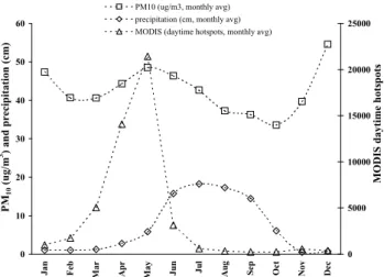
Though biofuel use is thought to occur mainly in rural ar-eas, it is possible that a significant amount of biofuel use also occurs in urban areas. Marley et al. (2009) reported that 70% of the carbon in the ambient MCMA aerosol was modern and ascribed this to open biomass burning and garbage burning. Garbage burning consumes some modern carbon, but also a large amount of plastics derived from fossil fuels. Some studies suggest a higher proportion of food waste for Mexi-can dumps than we estimated (Buenrostro and Bocco, 2003; Ojeda-Benitez et al., 2003; De la Rosa et al., 2009), which, if true, would not affect our %C, but could increase the frac-tion of modern carbon. However, indicafrac-tions are that much of the food waste may decompose before burning (Bernache-P´erez et al., 2001). If open burning was the dominant par-ticle source in the MCMA and ventilation rates were sim-ilar year round, the PM10levels should peak in March-May when nearly all the open biomass burning occurs. Instead the PM10data show at best a weak increase in PM10during these months (Fig. 6) indicating that a different, year round source of modern carbon could be “embedded” in the urban area. Possibilities include cooking fires and industrial biofuel use in addition to garbage burning.
4.3 Garbage burning impacts on the local-global atmosphere
We start this section by noting that the prevalence of open burning of garbage may be greater than commonly supposed even in developed countries. As noted earlier, it has been estimated that 12–40% of rural households in the US burn garbage in their backyards (USEPA, 2006). In the US, dump and landfill fires are reported at a rate of 8400 fires per year (TriData Corp., 2002). UK landfill operators surveyed by Bates (2004) estimated that, at any one time, deep seated fires are occurring at about 80 percent of landfills.
0 10 20 30 40 50 60
Jan Feb Ma
r
Apr Ma
y
Ju
n
Ju
l
Aug Se
p
Oct No
v
De
c 0
5000 10000 15000 20000 25000 PM10 (ug/m3, monthly avg)
precipitation (cm, monthly avg) MODIS (daytime hotspots, monthly avg)
PM
10
(
u
g/m
3) an
d
p
reci
p
it
a
ti
on
(
cm
)
M
O
D
IS daytime
hots
pots
Fig. 6.Time series of monthly average PM10(Pedregal RAMA
sta-tion 2003–2008 average, www.sma.df.gob.mx/simat/cambia base. htm); MODIS daytime hotspots for Mexico (2003-2008 aver-age, www.conabio.gob.mx); and monthly average precipitation for MCMA (see Sect. 4.2).
global source at 7.6 Tg/yr. Recent HCl profiles in the ma-rine boundary layer (Kim et al., 2008) may indicate that the sea salt dechlorination HCl source was over estimated. Our measurements indicate that the garbage burning HCl source may have been underestimated. In general, Keene et al. (1999) found that additional HCl sources totaling to 42 Tg/yr were needed to balance the HCl budget. With the above in mind, we propose that garbage burning may be a considerably more important tropospheric source of HCl than previously assumed. We also note that many of the other main HCl sources, such as sea salt and volcanoes, can often be associated with a humid environment and rapid removal of HCl (Tabazadeh and Turco, 1993). In dry environments, such as central Mexico where we measured water mixing ra-tios as low as 890 ppm, a larger fraction of freshly emitted HCl might react with OH to release Cl atoms. The latter would then react with NMOC. In any case, the HCl from garbage burning in dryer areas could have a longer lifetime and higher relative importance than the same amount of HCl emitted in wetter areas.
We examined data obtained by other MILAGRO investi-gators for possible evidence of garbage burning. A particles-into-liquid-sampler (PILS) deployed by Georgia Tech at the MILAGRO T1 ground station north of Mexico City during March 2006 observed chloride (up to 6 µg/m3)for most of the month, with an average of 0.5 µg/m3compared to 33 µg/m3 total PM2.5 (Greg Huey, personal communication, 2009). This translates to a mass ratio of 0.015. The average mass ra-tio of Cl−to the sum of particle species in our nascent smoke from garbage burning (Table 4) was 0.047±0.011. Thus, the PILS data suggests an approximate upper limit for the con-tribution of garbage burning to the PM2.5in the MC airshed that is similar to that from the Sb data (∼1/3). As with Sb
there are other Cl sources that could lower the garbage burn-ing contribution such as agricultural fires, brick makburn-ing kilns (Table 4) and volcanoes (e.g. Burton et al., 2007). We note that 3 of the 4 landfills we sampled are within ∼35 km to the west, north, and east of the T1 site (Table 1). We also note that EFCl−for brick kiln 1 was high and that this kiln is only ∼20 km west of T1. In addition, brick kiln 1 was one of many brick kilns in the region. Reff et al. (2009) list a number of source profiles with high Cl−/PM2.5 ratios in-cluding solid waste combustion, agricultural burning, vari-ous types of metallurgy, and other (less common?) industrial processes. Moffet et al. (2008) assigned much of the particu-late Cl−in the MCMA to waste incineration based partly on a lack of correlation between particle Cl−and SO2, which is often produced by metallurgy and partly on a similarity of the ambient profile to the profile for waste incineration, which is known to occur in northern Mexico City.
We also looked for evidence of chlorine atom chemistry in the hydrocarbon ratios measured by whole air sampling. A plot of i-butane versus n-butane for 62 canister samples collected from both airborne and ground based sampling lo-cations in and around MCMA gave an average i-butane/n-butane ratio of 0.33 (r2=1.00, Don Blake, Barbara Barlett, personal communication, 2009). This is consistent with min-imal chlorine atom oxidation of alkanes in the air sampled (Kim et al., 2008).
We make two other general points about garbage burning. More work is needed to measure other chlorinated emissions from burning refuse, including CH3Cl, which is also a pro-posed biomass burning tracer (Lobert et al., 1991). Sec-ondly, PVC (the primary source of HCl in garbage burn-ing emissions) is also the most important predictor of dioxin emissions from the open burning of domestic waste (Neu-rath, 2004), so removing PVC from the waste before burning should have multiple benefits.
5 Conclusions