Improving Sharpe Ratios and Stability of Portfolios by Using a Clustering Technique

Improving Sharpe Ratios and Stability of

Portfolios by Using a Clustering Technique

Jin Zhang

Dietmar Maringer

Abstract—This paper proposes a method which combines a clustering technique with asset alloca-tion methods, to improve portfolio Sharpe ratios and weights stability. The portfolio weights are com-puted based on cluster members and cluster port-folios, which are decided by an optimal cluster pat-tern. The optimized cluster pattern tells the belong-ing of assets to particular clusters, which is identified by using a population-based method, i.e. the Differ-ential Evolution, subject to maximizing the Sharpe ratio of terminal portfolios. We employ two differ-ent asset allocation methodologies, i.e. the mean-variance Markowitz allocation and the parameter-free equal weights allocation, with the Financial Times and Stock Exchange market and Dow Jones Industrial Average market data, to study the clustering impact on Sharpe ratio and weights instability of the terminal portfolios. As experimental results suggest that, the terminal portfolios from the clustered markets have higher Sharpe ratios than that without clustering. Furthermore, as a side effect of the clustering, the terminal portfolio weights become more stable than that in the non-clustered markets. Portfolio man-agers may cluster their assets with the Sharpe ratio criterion before distributing asset weights to improve portfolio weights stability and risk-adjusted returns.

Keywords: Clustering Optimization, Asset Allocation, Sharpe Ratio, Portfolio Stability, Differential Evolu-tion

1

Introduction

At the Markowitz efficient frontier, an efficient portfolio yields higher return than other portfolios given a same risk level. However, two elements in the Markowitz anal-ysis, i.e. the assets expected returns and covariance can hardly be predicted precisely using historical data, due to errors from estimation procedure and noise in finan-cial data itself. Furthermore, the investors who man-age large portfolios containing hundreds of assets, tends to face the ‘information deficit’ problem when historical

∗_{Centre for Computational Finance and Economic Agents,}

Uni-versity of Essex, United Kingdom. Email:[email protected]. The author gratefully acknowledges the financial support from the EU Commission through MRTNCT2006034270 COMISEF for attend-ing this conference.

†_{Faculty of Economics and Business Administration, University}

of Basel, Switzerland. Email:[email protected]

data has limited observations leading insufficient degrees of freedom in estimating the two elements. The litera-ture suggests several approaches to reduce or avoid the error and noise impact on portfolios. For example, to re-duce the error impact on the output stability after the variance-covariance matrix inversion, Harris and Yilmaz [1] combine the return-based and range-based measures of volatility to improve the estimator of multivariate con-ditional variance-covariance matrix. Some investors just ignore the mean and variance measures and turn in favor of the equally weighted investment strategy, or the so-called 1/N rule. For example, Windcliff and Boyle [2] pro-pose that 1/N rule should be optimal in a simple market where the assets are indistinguishable and uncorrelated. Benartzi and Thaler [3] discuses the 1/N puzzle in the context of asset allocation decision in a contribution sav-ing plan. In the research by DeMiguelet al. [4], the 1/N strategy is found outperforming other thirteen allocation models in terms of the Sharpe ratio, certainty-equivalent return and turnover. This paper proposes a method that introduces clustering to asset allocation procedure, to re-duce the negative impacts from the estimation errors and noise on the constructed portfolios.

portfolio. The terminal asset weights are decided by two parts, the cluster portfolio weights and cluster member weights. Three asset allocation methods are employed for the clustering study: the so-called naive 1/N allocation, the Markowitz minimum variance portfolio (MVP) allo-cation and the modified Tobin tangency portfolio alloca-tion. A population-based evolutionary method, the Dif-ferential Evolution (DE) is employed to tackle the clus-tering problem.

The paper is organized as follows. Section 2 introduces the clustering optimization problem, the data for empir-ical experiments, and the heuristic approach to solve the complex clustering optimization problem. Section 3 pro-vides experimental results and discussions, and Section 4 draws the concluding remarks.

2

The Asset Allocation Model

2.1

The Optimization Problem

The optimization problem is to identify an optimal clus-tering pattern setC, which is an union of optimal subsets

C1,C2, ...,CG. The terminal portfolio computed based on

the optimal pattern yields higher in-sample Sharpe ratio than that are computed by using other patterns with a same cluster number G. The optimization objective of the clustering problem can be expressed as follows:

max C SR=

¯

rp−r¯f

σp

, (1)

where SR represents the Sharpe ratio, C is the optimal partition set, ¯rp is the average return of the portfolio, ¯rf

is an estimate of the risk-free return, andσpis a measure

of the portfolio risk over the evaluation period.

When we apply clustering techniques to segment equity markets, there are several clustering constraints must be satisfied. G is the number of subsets in cluster set C

with a value range 1 ≤ G ≤ N, and N is the number of market assets. When Gis set at 1 orN, we have the non-clustered market. The union of segmented markets contains all market assets, and there is no intersection between two different clusters. If we denoteCgas theg-th

subset of assets andMas market assets, the constraints can be expressed as:

[

C=M, (2)

Cg∩ Cj =∅, ∀g6=j. (3)

To avoid the cases that one single cluster contains too many assets or an empty cluster exists, we impose cardi-nality constraints to cluster size, which are related to the cluster number G; if we let ˜Nmin

and ˜Nmax

denote the minimum and maximum asset number in a cluster, the

constrains are described as follows:

˜

Nmin

≤

N

X

s=1

Is∈C_g ≤N˜

max

∀g∈G, (4)

where Is∈C_g = (

1 ifs∈ Cg,

0 otherwise, (5)

with (

˜

Nmin

=⌈N 2G⌉,

˜

Nmax

=⌈3N 2G⌉.

(6)

When we apply asset allocations to construct portfolios, we impose weight constraints to the cluster members and cluster portfolios: the sum of cluster member weights in a cluster, and the sum of cluster portfolio weights should be equal to 1, respectively. In addition to that, depending on the asset allocation allowing short sales or not, we have positive or negative weights constraints. If we let

wg denote the weight of gth cluster portfolio, and wg,s

denote the weight of cluster member sin clusterCg, the

constraints are described as follows:

G

X

g=1

wg= 1, and

X

s∈C_g

wg,s= 1, (7)

with either

wg≥0, wg,s

(

≥0 ∀s, g:s∈ Cg

= 0 otherwise , (8)

or

−∞< wg<+∞, wg,s

(

∈(−∞,+∞) ∀s, g:s∈ Cg

= 0 otherwise . (9)

The terminal weight of an assetsis denoted byw_es, which

is the product of the cluster portfolio weight wg and the

cluster member weightwg,s,

e

ws=wg·wg,s ∀g:s∈ Cg. (10)

Thus the reward rp and risk σp of the portfolio can be

described as:

rp= G

X

g=1

wgrg= G

X

g=1

wg

X

s∈Cg

wg,srs= N

X

s=1

e

wsrs, (11)

σp=

v u u t

N

X

s=1 N

X

k=1

e

wswekσs,k. (12)

whererg is the return of cluster portfolio,

rg=

X

s∈Cg

wg,srs, (13)

andσs,kis the covariance between asset sandk.

2.2

Asset Allocation Methods

This subsection introduces three asset allocation methods which include the naive 1/N equal weights approach and two methods from the Markowitz mean-variance frame-work, to compute the cluster members weights wg,s and

cluster portfolio weightswg, respectively.

2.2.1 The 1/N˜ Allocation

We denote the equal weights allocation as 1/N˜ in this paper, to distinguish it from the traditional 1/N strat-egy. In the 1/N˜ allocating procedure, the cluster port-folio weights are decided by the cluster number G, and cluster member weights in a cluster are decided by the cluster size, i.e. the number of assets in the cluster. One should note that the cluster number G is manually as-signed, whereas the cluster size depends on the optimized pattern. Therefore, the cluster portfolio weights wg are

given by 1 over the cluster numberG, and cluster mem-ber weightswg,sin the subsetCg are computed by taking

1 over the number of cluster members♯{Cg}respectively,

wg=

1

G, (14)

wg,s=

1

♯{Cg}

= _PN 1

s=1Is∈Cg

. (15)

2.2.2 The Markowitz MVP Allocation

The MVP portfolio is the safest portfolio yielding the minimum variance at the Markowitz efficient frontier. We use quadratic programming to compute the cluster mem-ber weights, as well as the cluster portfolio weights:

max

w

λr′_{w−(1−λ)w}′_{Σw, (16)}

where w _{is either the cluster portfolio weights vector or}

cluster member weights vector, depending on whether the

r_{represents the expected return vector of cluster}

portfo-lios or cluster members, andΣis the variance-covariance matrix describing the correlation of cluster portfolios or cluster members. The λis set at 0 for a minimum vari-ance portfolio. The MVP allocation is a special portfolio at the Markowitz efficient frontier, which can be used as a proxy of other efficient portfolios, the cluster effect on the MVP is same as on the portfolios which locate on the efficient frontier. By setting the λ at a value range 0< λ <1, we have other efficient portfolios at the fron-tier.

2.2.3 The Modified Tobin Tangency Allocation

The third asset allocation is an extension from the To-bin’s original framework, which has an analytical solution

when short sales is allowed and a market safe rate is avail-able. In this study, the terminal portfolio is a tangency portfolio based on the cluster tangency portfolio returns, which are constructed using the assets returns in each cluster as inputs of the tangency allocation. The tan-gency allocation is also employed to construct the termi-nal portfolio based on the cluster portfolios return. The weights distribution from the tangency portfolio alloca-tion is described as follows:

A₌

· _r′

I′

¸

Σ−1£

r I ¤_≡

·

a b b c

¸

, (17)

w₌Σ−1£ _{r I} ¤ " 1

b−rf·c

−rs

b−rf·c

#

, (18)

whereI_{is the unity vector,rf is the risk-free rate.} r

rep-resents a vector of the expected returns of either cluster portfolios or cluster members,Σ is a variance-covariance matrix describing the correlation of cluster portfolios or cluster members, and correspondingly thew_{is the vector}

representing either cluster portfolio weightswgor cluster

member weightswg,s.

2.3

Optimization method

Most of the heuristic algorithms provide a way to con-struct possible solutions and find a best solution based on an evolutionary concept. The algorithms generate new solutions by recombining or modifying existing solutions, then select better solutions comparing with their prede-cessors given a function that measures how good each solution is. Heuristic methods have been applied by Gilli et al. [8], Gilli and Winker [9] to solve optimization prob-lems in finance and econometrics. Maringer [10] discusses constrained index tracking problems under investor loss aversion behavior.

Storn and Price [11] propose the Differential Evolution algorithm which is originally designed for the problems with continuous solution space. Here we propose an ap-plication of the algorithm to the clustering problem by using a variant of the original DE, which takes the advan-tage of diversity from noise to escape from local optima convergence and avoid premature convergence. Let the row vectors v_{p, p= 1...P denoted as solutions, for each}

current solutionp, a new solutionv_{cis generated by}

ran-domly choosing three different members from the current population (p1 6=p2 6=p3 6=p) with linear combination

their corresponding solution vectors in probability (π1),

otherwise the new solution inherits the originalpth solu-tion with probability 1−π1. In the standard DE, only the

population sizeP, the scaling factorFand the cross-over probability π1 need to be considered. The extra noise is

generated by adding normally distributed random num-ber vectors with the mean value being zero, to F value and the difference of two solution vectors1

, respectively.

The noise vectorsz1andz2have the property: they are random variables being zero in two probability π2 and

π3, otherwise following normally distribution N(0, σ12)

andN(0, σ2

2) respectively. Thus the modified linear

com-bination of the cross-over procedure is decried as follows:

vc[i] :=

½

vp[i] with probabiltiy 1−π1, or

vp1[i] + (F+z1[i])·(vp2[i]−vp3[i] +z2[i]),

(19) where π1 is the cross-over probability. We translate

the solutions to cluster sets by rounding them to the nearest integers, which tell the belonging of each asset. After the linear combination, the algorithm updates the elitist by using the solution with higher fitness, which is defined as the Sharpe ratio value in this paper. Whether a replacement of the solution of v_{p with}v_{c will process}

is decided from running a comparison, i.e. if the fitness value of v_{c is better than the one of} v_{p, the solution} v_{p is replaced by} v_{c, and the updated} v_{p exists in the}

current population. The process is repeated until a halting criterion met. The DE optimization procedure is described using the following pseudo code.

Algorithm 2.1: SR maximization(v_p)

1: randomly initialize population of vectorsv_p, p= 1...P;

2: while do

3: {generate new solutionsv′ p:}

4: for allcurrent solutionsv_{p, p=1...P} do

5: randomly pickp16=p26=p36=p;

6: vc[i]←vp1[i] + (F+z1[i])·

(vp2[i]−vp3[i] +z2[i]) at probabilityπ1;

7: orvc[i]←vp[i] at probability 1−π1;

8: interpretv_{cinto clustering partition;}

9: apply asset allocations to compute portfolio return andSR;

10: end for;

11: {select new population:}

12: for allcurrent solutions v_{p,p= 1...P} do

13: if Fitness(v_c)>Fitness(v_p)then; 14: v_{p ←}v_{c ;}

15: end if;

16: end for;

17: untilhalting criterion met.

2.4

Data and Implementation

We downloaded the adjusted daily prices of FTSE 100 stocks in the period from January 2005 to December 2006, and the prices of DJIA 65 stocks in the period from January 2003 to December 2004 from Yahoo.com. We computed the asset returns by taking log return of the daily price series. The in-sample experiments and out-of-sample experiments employ the first year and second year

data respectively. All experiments were performed on Matlab version 2007b and a Pentium 4 machine. Based on preliminary tests, the technical parameters of DE al-gorithm are set as follows. Population size is set at 100, although a general rule of thumb advises that the popu-lation size should be at least three times the number of variables, i.e. the size should be over 300. Instead of us-ing such a large population, we set the iteration number at a higher level, says 100 thousands times. The weight-ing factor F is set at 0.7, the crossover probability π1

is 50 percent. The parameters for generating the arti-ficial noise z1 and z2 are listed as follows: π2 = 70%,

π3= 30%,σ 2

1 = 0.1 andσ 2

2 = 0.03.

Portfolio stability issue has been widely discussed in the literature. The portfolio stability issue in this paper refer-ring how assets weights in a portfolio are sensitive to the errors in parameters inputs of an allocation. We use an instability measure which is proposed by Farrelly [12] to study weights changes due to estimation errors and noise subject to portfolio rebalance and transactions, which is defined as follows:

I= PN

i=1|wei,o−wˆi,e|

2 , (20)

wherew_ei,ostands for the asset weights in a portfolio that

is constructed based on the ‘true’ asset information, while ˆ

wi,e are the asset weights of the portfolio that are

com-puted by using the estimates containing errors and noise. In the instability experiments, we use the in-sample as-set returns as ‘the true’ asas-set information, and artificially generate the asset returns containing errors and noise by adding noise disturbances to assets which are randomly selected each time. We randomly choose 20% of the mar-ket assets each time, and set the noise expected value at 0, standard deviation at 0.5% in the experiment. We compute the instabilityI each time and take the average as the final instability after 10,000 times, while setting the cluster numberG at five different values, to tell the clustering impact on weights instability.

Since Sharpe ratio is widely used as a measure of portfo-lio performance, we use it to evaluate risk-adjusted return performance of the terminal portfolios over the both in-sample and out-of-in-sample period. The risk-free returnrf

is set at 0 because the experiments employ daily returns. Furthermore, we employ the two sample Kolmogorov-Smirnov (KS) test to statistically judge whether the ter-minal portfolio return distributions over the in-sample and out-of-sample period will be affected by the cluster-ing.

3

Computational Results

1 3 5 7 9 0.04

0.045 0.05 0.055 0.06

MVP Allocation

1 3 5 7 9

0.5 1 1.5 2

Modified Tobin Allocation

Total Cluster Number

Instability

Figure 1: Clustering Impact on Portfolio Weights Insta-bility, FTSE Market

1 3 5 7 9

0.06 0.08 0.1 0.12

MVP Allocation

1 3 5 7 9

0 20 40 60

Total Cluster Number

Instability

Modified Tobin Allocation

Figure 2: Clustering Impact on Portfolio Weights Insta-bility, DJIA Market

3.1

Portfolio Instability

Figure 1 and Figure 2 show the instability I which is computed from the simulated FTSE and DJIA returns containing the errors and noise in five cluster number cases, i.e. theGvalue being 1, 3, 5, 7 and 9. We studied the weights instability of portfolios from the MVP alloca-tion and Tobin tangency allocaalloca-tion using the FTSE and DJIA data respectively. We did not include the 1/N˜ allo-cation in this experiment since the alloallo-cation distributes weights independently of return means and variances. As the figure shows that, the instabilityI turns lower while we set the cluster numberGat larger values in the Tobin allocation case, and the weights instability from the MVP allocation is decreased further while the cluster number

G turns higher. The above evidences support that the portfolio weights from the clustered markets are less sen-sitive to the changes, or to the estimation errors and noise in the input parameters than that from the non-clustered markets.

3.2

Sharpe Ratios and Return Distribution

The second and third column in Table 1 provide the in-sample and out-of-in-sample Sharpe ratios, which are com-puted from the terminal portfolios returns based on the FTSE data using the three asset allocations. In the cases of using the 1/N˜ and MVP allocation, we find that the

Table 1: Sharpe Ratios and p-values, FTSE Market

SR(I) SR(O) p-values 1/N˜

G=1 0.159 0.077 0.095

G=3 0.207 0.079 0.053

G=5 0.213 0.078 0.041

G=7 0.214 0.075 0.041

G=9 0.220 0.079 0.032

MVP

G=1 0.155 0.083 0.008

G=3 0.207 0.085 0.008

G=5 0.230 0.082 0.006

G=7 0.239 0.081 0.012

G=9 0.245 0.076 0.012

Tobin

G=1 0.622 0.073 0

G=3 0.610 0.064 0.001

G=5 0.610 0.082 0.002

G=7 0.611 0.088 0.001

G=9 0.612 0.066 0.001

out-of-sample Sharpe ratios are increased by 0.25% when the cluster number is set at 3 respectively. In the mod-ified Tobin allocation case, the out-of-sample Sharpe ra-tio is increased by 20% when the cluster number G is set at 7. The fourth column in Table 1 provides the p-values from the K-S test. According to the p-values, the test rejects the hypothesis that the in-sample returns and out-of-sample returns follow a same distribution at a 10% confidence level. Surprisingly, the non-clustered cases from the three allocations have the p-values less than 10%, which indicates a structural break happened in the FTSE market between 2005 and 2006. To reconcile that the clustering improves the Sharpe ratio of terminal portfolios, we shall provide the experimental results using a different market data in different periods.

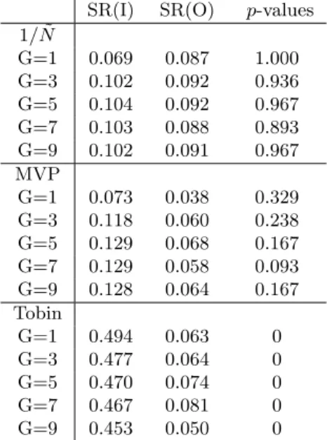
Table 2: Sharpe Ratios and p-values, DJIA Market

SR(I) SR(O) p-values 1/N˜

G=1 0.069 0.087 1.000

G=3 0.102 0.092 0.936

G=5 0.104 0.092 0.967

G=7 0.103 0.088 0.893

G=9 0.102 0.091 0.967

MVP

G=1 0.073 0.038 0.329

G=3 0.118 0.060 0.238

G=5 0.129 0.068 0.167

G=7 0.129 0.058 0.093

G=9 0.128 0.064 0.167

Tobin

G=1 0.494 0.063 0

G=3 0.477 0.064 0

G=5 0.470 0.074 0

G=7 0.467 0.081 0

G=9 0.453 0.050 0

4

Conclusion

This paper presents a new asset allocation model that combines a clustering technique with asset allocation methods to improve portfolio Sharpe ratios and portfolio weights stability. Using the Differential Evolution algo-rithm, we identify optimal clustering patterns in different cluster number cases, which contribute to higher Sharpe ratios and lower portfolio instability than that of port-folios from the non-clustered markets over the both in-sample and out-of-in-sample period. Market practitioners may cluster assets before they distribute portfolio weights when they have desires to improve portfolio weights sta-bility and risk-adjusted returns. In future research, we shall discuss the Differential Evolution stability and ef-ficiency, in the comparison with that of other evolution-ary methods, such as Threshold Accepting and Simulated Annealing while tackling the clustering problem, since the Differential Evolution is originally designed for problems with continuous solution space rather than the discrete solution space.

References

[1] Harris, Richard DF., Yilmaz, Fatih., “Estimation of the Conditional Variance - Covariance Matrix of Re-turns Using the Intraday Range”, Working papers, XFi Centre for Finance and Investment, 2007

[2] Windcliff, Heath. Boyle, Phelim P., “The 1/N Pen-sion Investment Puzzle”,North American Actuarial Journal, V8, pp. 32–45, 2004

[3] Benartzi, Shlomo. Thaler, Richard H., “Naive di-versification strategies in defined contribution

sav-ing plans”, The American Economic Review, V91, pp. 79–98, 2001

[4] DeMiguel, Victor. Garlappi, Lorenzo. Uppal, Ra-man., “Optimal versus Naive Diversification: How Inefficient Is the 1/N Portfolio Strategy?”, Review of Financial Studies, Forthcoming

[5] Pattarin, Francesco. Paterlinib, Sandra. Minervac, Tommaso., “Clustering financial time series: an ap-plication to mutual funds style analysis”, Computa-tional Statistics & Data Analysis,V47, pp. 353–372, 2004

[6] Lisi, Francesco. Corazza, Marco., “Clustering Finan-cial Data for Mutual Fund Management”, in Math-ematical and Statistical Methods in Insurance and Finance, Chapter 20, pp. 157–164, Springer, 2008

[7] Brucker, Peter., “On the complexity of cluster-ing problems”, in Optimization and Operations Re-search, Chapter 2, pp. 45–54, Springer, 1977

[8] Gilli, Manfred., Maringer, Dietmar., Winker, Peter., “Applications of Heuristics in Finance”, inHandbook on Information Technology in Finance, Chapter 26, pp. 635–653, Springer, 2008

[9] Gilli, Manfred., Winker, Peter., “A Review of Heuristic Optimization Methods in Econometrics”, Working papers, Swiss Finance Institute Research Paper Series, No. 8 –12, 2008

[10] Maringer, Dietmar., “Constrained Index Tracking under Loss Aversion Using Differential Evolution”, in Natural Computing in Computational Finance, Chapter 2, pp. 7–24, Springer, 2008

[11] Storn, R., Price, K., “Differential evolution – a simple and efficient heuristic for global optimiza-tionover continuous spaces”, Journal of Global Op-timization,V11, pp. 341–359, 1997