Fast and robust optimization approaches for pedestrian detection

VICTOR HUGO CUNHA DE MELO

FAST AND ROBUST OPTIMIZATION APPROACHES

FOR PEDESTRIAN DETECTION

Dissertação apresentada ao Programa de Pós-Graduação em Ciência da Com-putação do Instituto de Ciências Exatas da Universidade Federal de Minas Gerais como requisito parcial para a obtenção do grau de Mestre em Ciência da Com-putação.

O

: W

R

S

C

: D

M

VICTOR HUGO CUNHA DE MELO

FAST AND ROBUST OPTIMIZATION APPROACHES

FOR PEDESTRIAN DETECTION

Dissertation presented to the Graduate Program in Computer Science of the Uni-versidade Federal de Minas Gerais in par-tial fulfillment of the requirements for the degree of Master in Computer Science.

A

: W

R

S

C

-A

: D

M

c

2014, Victor Hugo Cunha de Melo. Todos os direitos reservados.

Melo, Victor Hugo Cunha de

M528f Fast and Robust Optimization Approaches for Pedestrian Detection / Victor Hugo Cunha de Melo. — Belo Horizonte, 2014

xxvi, 62 f. : il. ; 29cm

Dissertação (mestrado) — Universidade Federal de Minas Gerais

Orientador: William Robson Schwartz Coorientador: David Menotti

1. Computação Teses. 2. Visão por Computador -Teses. 3. Filtragem Aleatória. 4. Partial Least Squares. 5. Variable Importance on Projection. 6. Detecção de Pedestres. I Orientador. II Coorientador. Título.

Acknowledgments

First and foremost, I would like to express my gratitude to my advisor William Schwartz. From the beginning, William has always been there to listen and to ad-vise me. William’s enthusiasm, knowledge, and patience has always been a great inspiration to me. He has patiently helped me in refining my inarticulate ideas, teaching me what questions should be asked and how to express in scientific com-munication. He has been a great advisor, a mentor, and a friend. I have learned a lot under his guidance.

A special thanks goes to my coadvisor, David Menotti, who has always been an inspiration to me. David has always been a friend, supporting me and pushing me since my undergraduation. During this Master’s, David provided insightful thoughts, helping me everytime I thought I had reached a dead end. Thank you for inspiring me the interest for computer science and computer vision, and to pursue the academic career.

I would like to thank the Master’s thesis committee, Cláudio Rosito, Jefferson Santos, and Mario Campos. Thank you for carefully reviewing the text and for your insights on how this work could be improved.

During this Master’s, I have counted on the assistance of several friends. Thank you to my colleague Samir. Without him, this work would not be possi-ble. To my long time friends, Antonio Carlos and Suellen, who always supported me. To the SSIG group: Artur, Cássio, César, Cristiane, Jéssica, Ricardo, and all the members who were part of it, for the insightful discussions and the fun moments. To the friends I made in Verlab: Balbino, Cláudio, Douglas, Drews, Elerson, Erick-son, Fernando, and Vinicius, thank you for presenting me a whole new world and for making my transition more smoothly. To the PPGCC secretariat, who always at-tended me kindly and patiently. Finally, I would like to specially thank my roomate, Fernando, for being a great friend and making everything more amusing.

Minas Gerais Research Foundation - FAPEMIG (APQ-01294-12), and I would like to express my gratitude to them.

In conclusion, I would like to thank my parents Sebastião Porfírio and Ana Vera, my first advisors. Thank you for being the best parents that I could ever have. My brother Caio Hess, my first friend and colleague, thank you for always support-ing me. And my final words go to my love, Mariana. Mariana probably suffered the most, watching closely my sleepless nights, patiently skipping weekends and vacations. She was also there to share with me the good moments, making this ride more joyful. I cannot express how grateful I am for everything you did for me.

Abstract

The large number of surveillance cameras available nowadays in strategic points of major cities provides a safe environment. However, the huge amount of data provided by the cameras prevents its manual processing, requiring the application of automated methods. Among such methods, pedestrian detection plays an im-portant role in reducing the amount of data by locating only the regions of interest for further processing regarding activities being performed by agents in the scene. However, the currently available methods are unable to process such large amount of data in real time. Therefore, there is a need for the development of optimization techniques. Towards accomplishing the goal of reducing costs for pedestrian detec-tion, we propose in this work two optimization approaches. The first approach con-sists of a cascade of rejection based on Partial Least Squares (PLS) combined with the propagation of latent variables through the stages. Our results show that the method reduces the computational cost by increasing the number of rejected back-ground samples in earlier stages of the cascade. Our second approach proposes a novel optimization that performs a random filtering in the image to select a small number of detection windows, allowing a reduction in the computational cost. Our results show that accurate results can be achieved even when a large number of detection windows are discarded.

Resumo

O grande número de câmeras de vigilância hoje em dia disponíveis em pontos es-tratégicos das principais cidades fornece um ambiente seguro. No entanto, a enorme quantidade de dados geradas por estas câmeras impede o processamento manual, exigindo a aplicação de métodos automatizados. Entre estes métodos, a detecção de pedestres desempenha um papel importante na redução da quantidade de da-dos por localizar apenas as regiões de interesse para o tratamento posterior sobre as atividades a serem realizadas pelos agentes na cena. No entanto, os métodos de detecção de pedestres disponíveis atualmente são incapazes de processar tal quanti-dade de dados em tempo real. Portanto, é necessário utilizar técnicas de otimização para permitir a detecção em tempo real, mesmo quando grandes volumes de dados têm de ser processados. Para cumprir a meta de redução de custos para a detecção de pedestres, este trabalho propõe duas abordagens de otimização. A primeira abordagem consiste em uma cascata de rejeição baseada no método Partial Least Squares(PLS) e no método deVariable Importance in Projection(VIP), combinada com a propagação de variáveis latentes através dos estágios. Os resultados mostram que o método reduz o custo computacional, aumentando o número de amostras perten-centes ao fundo rejeitadas nos estágios iniciais da cascata. A segunda abordagem consiste em uma otimização baseada em uma filtragem aleatória na imagem para descartar um grande número de janelas de detecção rapidamente, permitindo uma redução do custo computacional. A avaliação experimental demonstra que pode ser obtido uma grande acurácia, mesmo quando um grande número de janelas de detecção é descartado.

List of Figures

1.1 Panoptes: an example of a smart surveillance system. . . 2

1.2 Example of holistic and part-based methods. . . 4

1.3 Looking at people and applications [Schwartz, 2012a]. . . 5

1.4 Example of car with a pedestrian protection system. . . 6

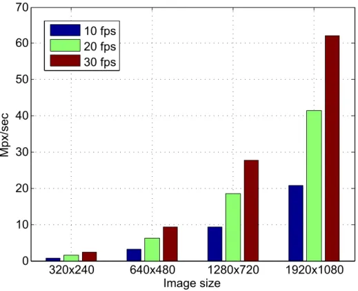
1.5 Amount of data recorded by a single camera at different frame rates and resolutions. . . 7

2.1 Illustration of HOG computation. . . 10

2.2 Example of a deep learning model. Source: Ouyang and Wang [2013]. . . 12

2.3 Part-based pedestrian model and detections. . . 14

2.4 Scheme of a general pedestrian detector. We propose optimizations re-lated to both steps of detection window generation and classification. . . 16

2.5 Example of a cascade of rejection. The i-th stage is composed of an en-semble of weak classifiers, creating a strong classifierH_i. Along with the ensemble, a stage has a thresholdθito reject or propagate a window. . . 18

2.6 Example of a GPU’s architecture and feature extraction. . . 20

2.7 An example of saliency detector. From left to right, the original image; the saliency map; and candidate regions in the saliency map. . . 22

3.1 Fluxogram describing the general steps of the optimization methodology proposed in this work. The balloon represents our proposed approach, divided into two smaller steps, namely, random filtering combined with location regression (Section 3.2), and the PLS Cascade (Section 3.3). . . . 27

3.2 Sliding window algorithm. A detection window scans the input image in all possible locations. . . 28

3.4 Mean number of detection windows covering a pedestrian in the INRIA dataset as a function of the percentage of randomly selected windows. As standard approach to determine whether a pedestrian is covered by a detection window [Dollar et al., 2012], we consider that a window A covers a ground-truth windowBwhen their intersection divided by their union (Jaccard coefficient) is greater than 0.5. . . 31 3.5 Examples of sample generation used in the learning phase of the location

regression. . . 33 3.6 Real example of performing location regression to adjust the detection

window location. . . 34 3.7 Overall layout of the proposed PLS cascade using Partial Least Squares

with latent variable propagation and Variable Importance on Projection (VIP) for feature ranking. . . 35 3.8 Testing phase. The detection window is evaluated through each stage

of the cascade. If the score of a detection window is higher than the rejection thresholdθi, it triggers the classifier of the next stage; otherwise,

it is rejected. This procedure repeats until the test sample reaches the last stage. When computing the regression, PLS gerenates a set of latent variablesT_i, which are propagated to the subsequent stages. . . 36 4.1 Positive training samples for the INRIA Person data set, normalized to

64×128 pixels. . . 40 4.2 Achievable recall as a function of the number of selected windows,

eval-uated on the INRIA data set (RF: random filtering). . . 42 4.3 Achievable recall as a function of the number of selected windows,

eval-uated on the INRIA data set (RF: random filtering, LR: location regression). 43 4.4 Variance of the random filtering and location regression. . . 44 4.5 Horizontal prediction of location regression when a detection window

moves away from a pedestrian. x-axis represents the horizontal move-ment, while they-axis presents the absolute error regarding the ground-truth. . . 45 4.6 Vertical prediction of location regression when a detection window

moves away from a pedestrian. x-axis represents the vertical movement, while they-axis presents the absolute error regarding the ground-truth. . 45 4.7 Recall achieved at 1 FPPI when the selected detection windows are

pre-sented to the PLS detector. The PLS detector is shown as line because it is executed with 100% of the detection windows (without filtering). . . . 46

4.8 Histogram of the distribution of the pedestrian according to the image coordinates in thexandyaxes. . . 48 4.9 Cumulative rate of discarded samples as a function of the stages,

re-ported for different setups and methods. The setup referred to as PLS cascade is composed of VIP once and incremental propagation of latent variables. . . 50 4.10 Results achieved with different setups and methods, reported in a

detec-tion error tradeoff plot. . . 51 4.11 Percentage of projections performed by each method, normalized by the

List of Tables

List of Abbreviations

PLS Partial Least Squares

PCA Principal Component Analysis

FPS frames per second

FPPW False Positives Per Window

FPPI False Positives Per Image

PPS Pedestrian Protection Systems

SVM Support Vector Machines

VIP Variable Importance on Projection

HOG Histograms of Oriented Gradients

ADAS Advanced Driver Assistance Systems

DET Detection Error Tradeoff

RF Random Filtering

Contents

Acknowledgments ix

Abstract xiii

Resumo xv

List of Figures xvii

List of Tables xxi

List of Abbreviations xxiii

1 Introduction 1

1.1 Motivation . . . 3 1.2 Dissertation’s Goal . . . 6 1.3 Contributions . . . 7 1.4 Dissertation Organization . . . 8

2 Related Work 9

2.1 Pedestrian Detection Approaches . . . 9 2.1.1 Holistic-Based Detectors . . . 9 2.1.2 Part-Based Detectors . . . 13 2.2 Computational Cost Issues . . . 15 2.3 Optimization Approaches . . . 16 2.3.1 Cascade of Rejection . . . 17 2.3.2 Parallelization and GPUs . . . 19 2.3.3 Region of Interest Filtering . . . 21

3 Methodology 25

3.2 Random Filtering and Location Regression . . . 28 3.2.1 Random Filtering . . . 28 3.2.2 Location Regression . . . 31 3.3 Partial Least Squares Cascade . . . 33 3.3.1 Partial Least Squares Analysis . . . 34 3.3.2 PLS Cascade . . . 37

4 Experimental Results 39

4.1 Data Sets . . . 39 4.2 Random Filtering and Location Regression . . . 40 4.2.1 Experimental Setup . . . 41 4.2.2 Ground-truth Comparison . . . 42 4.2.3 Location Regression . . . 43 4.2.4 Pedestrian Detector . . . 44 4.2.5 Computational Cost . . . 47 4.2.6 Pedestrians’ Distribution . . . 47 4.3 PLS Cascade . . . 48 4.3.1 Experimental Setup . . . 49 4.3.2 Baseline Cascade . . . 49 4.3.3 Application of the VIP . . . 49 4.3.4 Propagation of Latent Variables . . . 50 4.3.5 Comparisons . . . 51 4.4 Discussion and Remarks . . . 53

5 Conclusions 55

5.1 Future Works . . . 55

Bibliography 57

Chapter 1

Introduction

V

suffered a huge growth due to the dropping prices of the cameras and the in-creasing network connectivity [Porikli et al., 2013]. Nowadays, we have a grow-ing availability of visual data captured by surveillance cameras, which provides safer environments for people whom attend monitored environments. However, the large number of cameras to be monitored and consequently the large number of im-ages that must be interpreted, precludes an effective manual processing and require a significant number of people dedicated to analyzing visual data. The ubiquity of video surveillance is advantageous for protection, but it is harder to monitor.

Although the large amount of visual data may provide more secure environ-ments, their analysis becomes challenging when performed manually. In addition, most of the data do not present interesting events from the surveillance standpoint, turning it into a repetitive and monotonous task for humans. Hence, automatic un-derstanding and interpretation of activities performed by humans in videos show great interest because such information can assist the decision making process of security agents.

Most surveillance systems usually employ human operators to monitor activ-ities of interest. However, human operators are more susceptible to fatigue after a certain time of video monitoring. Hampapur et al. [2003] show that after 20 minutes of watching and evaluating monitor screens, the operator’s focus weakens to well bellow acceptable levels. In addition, we cannot forget that operators are not always well-intentioned, such as recently happened on Araraquara (Brazil) in which the op-erators were using the surveillance cameras to inappropriately look at women1. On the other hand, smart surveillance tries to minimize these problems and can be used

2 CHAPTER 1. INTRODUCTION

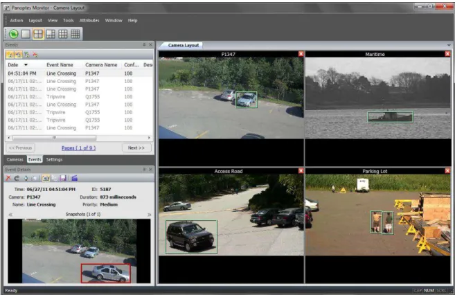
Figure 1.1. Panoptes: an example of a smart surveillance system, developed by intuVision. Source: http://www.intuvisiontech.com/products/panoptes. php.

to assist the operators, showing only relevant content instead of the full video.

Smart surveillance is defined by the employment of automatic video analy-sis technologies in video surveillance applications [Hampapur et al., 2003]. Smart surveillance systems can be designed to small processing tasks, such as detection of unusual events, or to more complex ones, such as semantic understanding of the activies happening on a video. In addition, it may be used to assist surveil-lance operators to maintain their focus only on important events. For instance, Fig-ure 1.1 depicts an operating smart surveillance system, detecting pedestrians who are crossing dangerous regions, cars in parking lots, and ships. Regardless the range of operation of those systems, the first step is to detect the pedestrians’ position in an image, since they are the most important agents in the scene.

1.1. MOTIVATION 3

used to take preventive decisions to maintain the well being of people.

This work focuses on pedestrian detection, a subproblem of human detection. The term pedestrian detection differs from human detection in the range of poses a person may assume. We can distinguish them as the following. Human detection is more broad, including people in any pose, while pedestrian detection is restricted to bodies close to an upright position. Dalal and Triggs [2005] define pedestrian detection as “the detection of mostly visible people in more or less upright poses, usually standing.” For now on, we will only refer to pedestrian detection throughout this work. We focus on pedestrian detection because, besides of capturing the most important poses in video footages, pedestrians are the main agents interacting with the environment in surveillance videos. Hence, we define pedestrian detection as the following:

Definition 1.1 (Pedestrian Detection). Given an input image, a sequence or a video footage, the Pedestrian Detection problem consists of locating the position of all persons close to an upright pose, covering their exactly height and weight.

Pedestrian detection methods can be divided into two categories: holistic and part-based methods [Schwartz et al., 2009]. Holistic methods statistically analyze a detection window combined with the feature extraction to classify whether this win-dow contains a pedestrian or not (see Figure 1.2(a) for an example). On the other hand, part-based methodsconsist of a generative process where detected parts of the human body are combined based on a prior human model (Figure 1.2(b)).

Several challenges are faced by the pedestrian detection problem [Geronimo et al., 2010]. Among them, there are changes in appearance due to different types of clothing, illumination changes and pose variations, low quality of the data acquired, and the small size of the pedestrian, which makes the detection process harder. In addition, a large number of applications require a high performance and reliable detection results, outlining the need for efficient and accurate pedestrian detection approaches.

1.1

Motivation

4 CHAPTER 1. INTRODUCTION

(a) (b)

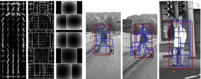
Figure 1.2. Example of holistic and part-based methods. (a) Holistic method. Source: Dalal and Triggs [2005]; (b) Part-based method. Source: Lin and Davis [2008].

tasks depend upon. Hence, pedestrian detection must be fast enough, otherwise the tasks depending on it will be executed after the events of interest have already happened and then being useless to take preventive actions. In addition, it must be accurate since the high-level tasks depends upon the data provided by detection (e.g., if poorly locations are used for action recognition, one might miss an action).

Real-time applications require accurate and fast answers regarding the pres-ence of a pedestrian to take preventive actions. The automotive industry and the scientific community, for example, are currently researching intelligent systems inte-grated into the vehicle aimed at anticipating accidents to avoid or lessen its severity. These systems are called Advanced Driver Assistance Systems (ADAS) [Geronimo et al., 2010], in which Pedestrian Protection Systems (PPS) play an important role. The goal of a PPS is to detect the presence of pedestrians in a specific region around the vehicle, as illustrated in Figure 1.4, in such way that the driver can be notified about this presence or an automatic preventive action is taken to stop the vehicle.

1.1. MOTIVATION 5

Feature Extraction

Background Subtraction

Pedestrian Detection

Pose Estimation

Tracking

Face

Recognition Reidentification

Action Recognition

Scene Description Video

Activity Recognition

Figure 1.3. Looking at people and applications [Schwartz, 2012a]. Background subtraction is shaded because it is optional to the execution of the other tasks.

rate. Nevertheless, the majority of pedestrian detection methods are not fast enough for these applications [Dollar et al., 2012]. Therefore, it is desirable the development of methods to significantly reduce the computational cost. One way of achieving that is to focus on optimization approaches.

GPU-6 CHAPTER 1. INTRODUCTION

Figure 1.4. Example of car with a pedestrian protection system. Source: http: //www.caradvice.com.au/.

such approaches still are not enough to achieve real time processing in most cases.

1.2

Dissertation’s Goal

In this work we study the pedestrian detection problem, focusing at reducing its computational cost. The problem we are tackling can be defined in the following question:

Dissertation’s Problem. How to reduce the computational cost of pedestrian detection methods while keeping a high accuracy?

1.3. CONTRIBUTIONS 7

323x243 643x483 1283x723 1923x1383 3

13 23 33 43 53 63 73

Image size

Mpx/

sec

13 fps 23 fps 33 fps

Figure 1.5.Amount of data recorded by a single camera at different frame rates and resolutions.

In our second approach, described in Section 3.3, we reduce the computational cost of the PLS Detector [Schwartz et al., 2009] by applying the Partial Least Squares (PLS) [Rosipal and Kramer, 2006] in a rejection cascade framework to reduce the number of projections and the amount of feature descriptors extracted (responsi-ble for the majority of the computational cost). Varia(responsi-ble Importance on Projection (VIP) [Wold et al., 1993] is applied to rank features according to their discriminative power, allowing the rejection of more samples in earlier stages of the cascade which effectively reduces the number of projections and extracted feature descriptors. In addition, this work also proposes the propagation of latent variables, estimated by PLS, from one stage to another, aiming at achieving high accuracy. The cascade resulting from the methodology described in this work is referred to asPLS Cascade.

1.3

Contributions

8 CHAPTER 1. INTRODUCTION

pedestrian detector;

• The application of Variable Importance on Projection (VIP) for feature ordering for fast training cascades of rejection;

• A new filtering approach, which can be applied on any sliding window based detector;

During the development of this work, we were awarded as one of the best works at the Seminar Week of the Graduation Program in Computer Science at Uni-versidade Federal de Minas Gerais. In addition, we have produced some technical papers which have been submitted for publication. The following list provides ref-erences to these documents.

• Melo, V., Leão, S., Campos, M., Menotti, D., and Schwartz, W. (2013). Fast pedestrian detection based on a Partial Least Squares Cascade. In IEEE International Conference on Image Processing.

• Melo, V., Leão, S., and Schwartz, W. (2013). Pedestrian Detection Optimization Based on Random Filtering. In Workshop of Works in Progress (WIP) at Confer-ence on Graphics, Patterns and Images (SIBGRAPI).

• Melo, V., Leão, S., Menotti, D., and Schwartz, W. (accepted). An Optimized Sliding Window Approach to Pedestrian Detection. In International Conference on Pattern Recognition.

1.4

Dissertation Organization

Chapter 2

Related Work

Several pedestrian detection approaches have been proposed in the past years. In this chapter, we review mainly works that focus on reducing the computational cost and improving the detection rate. Initially, Section 2.1 addresses the main pedestrian detection methods and the state-of-the-art solutions in the literature. Section 2.2 de-scribes the computational cost issue of pedestrian detection. Section 2.3 reviews different approaches employed for reducing the computational cost, including cas-cade of rejection and region of interest filtering, subjects directly related to our two solutions proposed in this work.

2.1

Pedestrian Detection Approaches

We present in this section the state-of-the-art on pedestrian detection methods based on Computer Vision. These methods may be divided into two classes, holistic and part-based [Schwartz et al., 2009]. We focus mainly on monocular detectors rather than stereo ones once stereo pairs of cameras are not always available, e.g, in surveil-lance systems.

2.1.1

Holistic-Based Detectors

dis-10 CHAPTER2. RELATEDWORK

Figure 2.1.Illustration of HOG computation.

criminative information due to the large size of whole body, when compared to the sizes of the parts [Schwartz et al., 2011].

Among these methods, Dalal and Triggs [2005] contributed with a remarkable work for allowing a large improvement on pedestrian detection and other object de-tectors as well. They proposed a new detector based on a novel feature descriptor1 called Histograms of Oriented Gradients (HOG) which was able to achieve better results than the top performers at that time, such as detectors based onwavelets [Vi-ola et al., 2003] and PCA-SIFT [Ke and Sukthankar, 2004]. The HOG is extracted from a detection window divided into cells of size 8×8. Each group of 2×2 cells is integrated into a block in a sliding fashion, making a dense grid of overlapping blocks [Zhu et al., 2006]. Next, the algorithm computes a histogram of oriented gra-dients for each cell, followed by a L2-norm with an optional clipping. Each block contains the concatenation of all its cells. We give details about this procedure on Figure 2.1. The HOG can be optimized by applying integral images [Viola and Jones, 2001], in which each histogram bin corresponds to an integral image. The HOG de-scriptor still is one of the most used and has inspired several others [Wang et al., 2009; Prisacariu and Reid, 2009; Dollár et al., 2009].

Based on integral images, Dollár et al. [2009] proposed linear and non-linear transformations to compute multiple registered image channels, called Integral Channel Features. Authors employed these descriptors into their CHNFTRS

2.1. PEDESTRIANDETECTIONAPPROACHES 11

tor. Using 6 orientation bins, 1 gradient magnitude, and 3 LUV color channels are enough to reach state-of-the-art results. In Dollár et al. [2010], it is proposed a fea-ture extraction that exploits the interpolation of feafea-tures in different image scales, significantly reducing the cost and producing faster detectors when coupled with cascade classifiers. The Integral Channel Featurehas demonstrated to be one of the fastest, yet simpler, feature descriptor, being used by several works. Our proposed approaches can also benefit from this feature descriptor since they are independent of the feature descriptors used.

Schwartz et al. [2009] noticed that using HOG by itself may lead to false posi-tives due to the spatial distribution of edge orientations. Thus, objects with a similar spatial distribution to pedestrians, such as trees and light poles, may be misclassi-fied as pedestrians. They observed that this problem can be avoided if one considers other important sources of information that inherently belong to pedestrians and do not belong to these false positives. The authors explored this insight proposing the use of information to complement the one extracted by HOG, such as cloth-ing homogeneity and skin color. This information set increases the feature space, making the problem intractable by conventional machine learning techniques, such as Support Vector Machines (SVM). Hence, Schwartz et al. applied the supervised statistical approach called Partial Least Squares (PLS) to project the feature vectors onto a smaller subspace, allowing the use of SVM and quadratic classifiers. Along with the detector, the authors also proposed the use of Variable Importance on Pro-jection, a feature selection tool based on PLS. The VIP provides a score for each feature, allowing to rank them according to their discriminative power in the PLS model [Schwartz et al., 2009]. This is important for our work because we employ it on the training phase of the cascade, allowing to considerably reduce the training computational cost and reduce a high number of detection windows on the early stages of the cascade.

Benenson et al. [2012b] proposed a monocular and, optionally, stereo detector with four incremental approaches. Their method is able to reach 50 FPS on a monoc-ular system and 135 FPS on its stereo form. The authors use CHNFTRS[Dollár et al.,

12 CHAPTER2. RELATEDWORK

Figure 2.2.Example of a deep learning model. Source: Ouyang and Wang [2013].

the search area, the authors employ depth information extracted by an estimation of stixels[Benenson et al., 2011] andground-plane.

Marin et al. [2013] proposed a combination of multiple local experts by means of a Random Forest ensemble. Each tree of the forest corresponds to a local expert, classifiers trained for feature vectors extracted from the same rectangular area across several windows. Their method works with rich block-based descriptors which are reused by the different experts of the ensemble. To obtain complementary and dis-criminant local experts, the authors employ a feature selection based on a random principle. They extractKrectangular areas with random values of width and height, and then the most discriminant ones are selected. They also show how to integrate the ensemble with a soft-cascade, in which the initial layer is compound of a number of trees and each following layer has an additional tree.

2.1. PEDESTRIANDETECTIONAPPROACHES 13

2.1.2

Part-Based Detectors

Besides holistic detectors, another approach to perform detection consists of mod-eling the pedestrians’ constituents into a part-based fashion. In general, part-based detectors consists of a bottom-up approach that first detects the parts of a pedestrian until it gradually matches the whole pedestrian’s body. They can be combined with a holistic detector, which is referred asrootwithin this context [Felzenszwalb et al., 2010b]. The body parts might be either real, such as head, torso, arms, and legs, or only body-inspired, in which the detection window is virtually splitted into regions corresponding to body parts. In addition, they can be assumed at fixed locations or searched in a range of allowed locations. The latter method, known as deformable, allows the detection of unseen poses during the training phase and the removal of misclassified parts [Geronimo and López, 2013].

Part-based detectors show better performance on high-resolution images and are more suitable to handle conditions such as pose variation and partial occlu-sions [Dollar et al., 2012]. However, they are harder to train because they often make use of latent information, which is hard to retrieve because most datasets do not have body parts’ annotations and it is daunting to make it manually [Felzen-szwalb et al., 2010b]. Because of these weakly labeled data, deformable models are often outperformed by models such as holistic on difficult datasets, containing low quality images.

Among the classical part-based detectors, Weber et al. [2000] and Fergus et al. [2003] proposed constellation structures that restrict parts of the body to a sparse set of localizations, determined by a keypoint detector. The constellations capture the geometric arrangement by using a Gaussian distribution. In contrast, pictorial structure models [Felzenszwalb and Huttenlocher, 2005] define a matching prob-lem whose body parts have an individual correspondence cost in a dense set of localizations. Amit and Trouvé [2007] employed a similar approach, but the authors consider explicitly as a appearance model with overlapping parts.

ap-14 CHAPTER2. RELATEDWORK

Figure 2.3.Part-based pedestrian model and detections. From left to right, HOG model of the root; HOG model of eight parts; spatial layout cost function of the parts (darker regions represents lower deformation cost); detections in Daimler A.G. dataset, shown boxes frame the detected root and parts. Source: [Geronimo and López, 2013], with kind permission of Springer Science+Business Media.

category [Schneiderman and Kanade, 2000].

Tosato et al. [2010] defined an hierarchy of overlapping parts with different size levels. The hierarchy is structured in such a way that the number of details is increased at each level. For example, the first level takes into account the full pedestrian’s body. In the second level, the authors split the candidate window into three virtually body-inspired partitions, which are head-shoulder, torso and legs. The third level considers seven parts, the head, left and right shoulders, arms and legs. The authors combine the full hierarchy, composed of 11 parts altogether, by means of an ensemble using LogitBoost and using covariance as feature.

Felzenszwalb et al. [2010b] proposed a discriminatively trained, multi-scale, and deformable part model for object detection. The method reveals to obtain com-petitive results for pedestrian detection as well. Their method includes both a root model covering the entire pedestrian and part models in higher resolution. As explained earlier, the training phase is harder for part-based detectors due to the lack of annotated parts. In that work, the authors presented a new methodology for learning parts from weakly-labeled data based on generalization of SVMs, re-ferred tolatent SVM, which handles latent variables such as part positions. In ad-dition, Felzenszwalb et al. [2010b] presented a new bootstrap method for data min-ing hard negative samples durmin-ing trainmin-ing. The final detector, LATSVM, showed

2.2. COMPUTATIONALCOST ISSUES 15

parts allows to compute a more precise location of the detected pedestrians, than when using only the root model. Moreover, an extension of this work is proposed by Park et al. [2010] to use multiresolution models, in which the method automat-ically switches to parts only at sufficiently high resolutions, since LATSVM scores

better within this scenarios.

2.2

Computational Cost Issues

As illustrated in Figure 2.4, a general pedestrian detector is commonly composed of the following steps. The first step generates a set of detection windows that sample an input image. The second step extracts a set of feature descriptors from each detec-tion window. Finally, in the third step, the feature vector of the detecdetec-tion windows are presented to a classifier, which will output high responses for those detection windows likely to contain pedestrians.

So far, we have reviewed several methods that addressed the pedestrian detec-tion problem. Such methods still present a high computadetec-tional cost related to two steps in common to every detector, namely, the feature extraction and the classifica-tion.

Feature extraction focuses on extracting relevant cues that better describe a given object. This step would not be necessary if we decided to use the image pixels by themselves. However, we cannot use pixel intensities solely since they are sub-ject to noise, changes in illumination, curse of dimensionality, among others. Hence, we employ feature extractors to compute measurements that are meaningful and in-variant to certain properties, such as localization and illumination [Trucco and Verri, 1998].

In the training phase, the classifier learns the pedestrian model from a set of feature descriptors extracted from several examples of pedestrians. In the testing phase, the algorithm repeats the procedure of extracting features from each detec-tion window, and then presents them to the classifier, which provides a confidence score for this sample. As a detector must extract features for every test sample, which can easily be more than 60,000 for a single 640x480 image, feature extraction is responsible for a considerably amount of the computational cost. Therefore, we are interested in extracting meaningful features for pedestrians, constrained by their low computational cost.

com-16 CHAPTER2. RELATEDWORK

Detection Windows

Feature Extraction

Input Image

Detected Pedestrians

Classifier

Figure 2.4. Scheme of a general pedestrian detector. We propose optimizations related to both steps of detection window generation and classification.

taking a set of labelled examples and using them to come up with a rule that will as-sign a label to any new example. In the general problem, we have a training dataset

(x_i,y_i); each of thex_i consist of the feature vector for the i-th sample, and they_i is a label giving the type of the object that generated the example [Forsyth and Ponce, 2011]. We need a classifier that best separates data into either pedestrian or back-ground classes. While using more complex functions might lead to better results, they also increase the computational cost. Thus, we must deal with the trade-off of the computational cost versus the detection rate. Moreover, if the detector must deal with high dimensional feature spaces, it might be necessary to reduce the number of dimensions. One may apply dimensionality reduction tools, such as Principal Component Analysis (PCA) and PLS, before presenting the sample to the classifier, which influences the computational cost, as well.

2.3

Optimization Approaches

2.3. OPTIMIZATION APPROACHES 17

the amount of data processed, which allows the extraction of fewer features and fewer samples, consequently reducing the computational cost. On the other hand, the optimization approaches resort to specialized hardware to speed up the compu-tation.

In this section, we explore the main optimization approaches for pedestrian detection, grouping them in three main categories:cascades of rejection(Section 2.3.1), parallelization and GPUs (Section 2.3.2), and filtering(Section 2.3.3) [Benenson et al., 2012b]. In addition to these categories, prior knowledgealso deserves mentioning. It takes advantage from information of the environment and the camera setup, such as ground plane estimation and fixed cameras, allowing to restrict the search area instead of scanning the full image. Since such approaches depend on the inherent characteristics of the data set, they are complementary to our work. Hence, we do not extend on this topic.

2.3.1

Cascade of Rejection

Rejection cascades are a widely employed approach to reduce the computational cost in object detection. They are composed of multiple stages, each one composed of a classifier or an ensemble of them. The most common cascade employs AdaBoost to build an ensemble of weak classifiers in each stage, as illustrated by Figure 2.5. They are trained by adding features until the target detection and false positives rates are met. A cascade of rejection may also be referenced by other names, such as cascade of classifiers [Bourdev and Brandt, 2005], since it has multiple succeeding classifiers; or even attentional cascade [Viola and Jones, 2001], as it focus attention on samples harder to classify.

18 CHAPTER2. RELATEDWORK

...

sample

Figure 2.5. Example of a cascade of rejection. The i-th stage is composed of an ensemble of weak classifiers, creating a strong classifierHi. Along with the ensemble, a stage has a thresholdθito reject or propagate a window.

The cascade framework was initially employed in face detection by Viola and Jones [2001]. In their seminal work, they proposed a face detector using this tech-nique by successively combining classifiers with increasing complexity by means of AdaBoost[Freund and Schapire, 1995] to build the cascade stages to allow rejection of a large amount of windows in early stages.

In the pedestrian detection domain, the rejection cascade was firstly used by Zhu et al. [2006] with the extraction of HOG features [Dalal and Triggs, 2005], resulting in detection rates comparable to the state-of-the-art of the literature at that moment with substantial speed improvement. However, the training time consid-erably increased since AdaBoost needs to select the most discriminative features to compose each of its weak classifiers.

Tuzel et al. [2007] improved the results obtained by Dalal and Triggs [2005] ap-plying low-level features including intensity, gradient, and spatial location along with a covariance matrix. As covariance matrices do not lie in a vector space, the authors applied LogitBoost classifiers combined with a rejection cascade that contains points lying on a Riemannian manifold. As an extension to Tuzel et al. [2007], Paisitkriangkrai et al. [2008] proposed a classification cascade that evaluates weak classifiers in a Euclidean space, instead of a Riemannian manifold, which re-sults in a faster method.

A cascade of classifiers was also employed to build deformable part mod-els. Felzenszwalb et al. [2010a] proposed a cascade of classifiers in which partial hy-potheses are eliminated by a sequence of thresholds determined by a set of positive examples, which theoretically guarantee the performance of this cascade method. The detection algorithm of the cascade for general classification models is formally defined by one grammar.

algo-2.3. OPTIMIZATION APPROACHES 19

rithm for soft-cascades. It computes thresholds to terminate the computation with no reduction in detection rate or increase in false positive rate on the training set.

Dollár et al. [2012] reduced the computational cost of their previous method [Dollár et al., 2010], reaching a speed detection of 35–65 FPS using the crosstalk cascades. In this cascade variation, the authors explore the correlations among the adjacent detection windows, introducing two opposite mechanism: de-tector excitation of promising neighbors and inhibition of inferior neighbors. Due to this communication between detectors, this method reaches a 4–30x speedup.

In general, we train one cascade of rejection for the domain of interest, e.g pedestrians or faces. However, the cascade may fail when presented to a different domain from the one learned. For instance, consider a cascade of classifiers trained for a domain of adult faces. This cascade might be unable to generalize the classifi-cation for baby faces. A common solution consists in training one cascade for each domain, i.e one cascade for adult faces and a second cascade for baby faces. Nev-ertheless, this is not scalable for a large number of data domains because it requires huge data annotation and computational effort. With this in mind, Jain and Far-fade [2013] proposed a cascade variation that easily allows the adaptation of a pre-trained cascade to a new similar domain, instead of training one for each domain from scratch. The solution requires a small number of labeled positive samples from a different yet similar data domain. The results are better than the baseline cascade and the one trained from scratch using the given training examples.

Different from the previous approaches, our detector, the PLS Cascade (de-scribed in Section 3.3), proposes a cascade of classifiers using a combination of PLS and variable selection approach VIP aiming at reducing the number of projections required by the PLS detector [Schwartz et al., 2009]. In addition, different from ap-proaches such as Viola and Jones [2001] and Zhu et al. [2006], the proposed cascade propagates information (without increasing the computational cost) to later stages to increase the discriminability of the classifiers instead of maintaining all feature descriptors as candidates during all stages. Our resulting approach is faster to train than the conventional cascades; the usage of the VIP allows to reject more samples in the earlier stages, and the computational cost of the PLS Detector is considerably reduced.

2.3.2

Parallelization and GPUs

20 CHAPTER2. RELATEDWORK

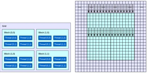
Figure 2.6. Example of a GPU’s architecture and feature extraction. Left image illustrates the thread architecture, while the right one exemplifies HOG extrac-tion using GPU. Each vertical arrow represents one thread and the direcextrac-tion they follow to process the pixels in the cell. Source: Prisacariu and Reid [2009].

niques allows to significantly increase the performance. Although Moore’s Law predicts that processing capacity doubles every two years, the processing speed for a single CPU is apparently stuck for a few years, making it unpractical to depend only on such architecture. However, Moore’s Law is still valid for highly paralleliz-able architectures, such as CPUs with multiple cores and GPUs [Leibe et al., 2008]. Thus, new methods for object detection must explore the capabilities of this growing architecture.

2.3. OPTIMIZATION APPROACHES 21

GPU to calculate integral images and filter evaluation, reaching 35 frames per sec-ond in resolutions up to 1960×1080 and using the sliding window approach with shifting of one pixel.

Although parallelization and GPU algorithms are not addressed by this work, our proposed approaches may benefit from them since they are complementary. For example, we could employ feature extraction using GPU, which would allow a significantly speedup to our method.

2.3.3

Region of Interest Filtering

Filtering regions of images consists in removing elements that do not belong to the targeted object, reducing the region of search and keeping only potential objects of interest, as illustrated in Figure 2.7. With smaller searchable regions, a robust clas-sifier is applied onto a smaller number of windows. Therefore, instead of using this classifier in the entire image, it is applied only in small regions, reducing the com-putational cost of detection. Several methods address the aforementioned problem induced by dense search in sliding window approaches. Some proposed heuristics evaluate windows in fixed sizes, which are subsampled for certain strides [Dalal and Triggs, 2005; Ferrari et al., 2008]. Depending on the stride, one might obtain a more sparse or dense sampling of the image. For example, larger strides yields more sparse sampling of the image.

Focusing on searching only promising regions of the image, Lampert et al. [2008] proposed a method to perform object localization relying on a branch-and-bound approach that finds the global optimum of a quality function over every possible subimage. It returns the same object locations that an exhaustive sliding window approach would, but requiring fewer classifier evaluations than there are candidate regions in the image, typically running in linear time or faster in function of the number of images. Related to this work, Lampert [2010] described a divide and conquer method to accelerate the evaluation of classification cascades for object detection. A set of candidate regions, in contrast with individuals regions, permit a large number of potential locations to be discarded, reducing the computational cost compared to other cascade strategies for object detection.

22 CHAPTER2. RELATEDWORK

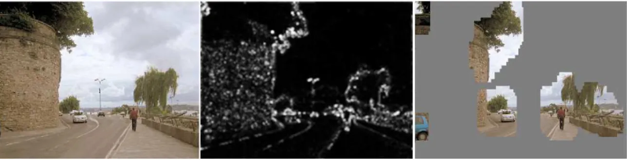
Figure 2.7. An example of saliency detector. From left to right, the orig-inal image; the saliency map; and candidate regions in the saliency map. Source: Silva Filho et al. [2012].

the image into regions based on their similarities. To find the most probable win-dow to contain a salient object, it is employed the difference among regions given their LAB color histograms and spatial distances.

To detect objects in different sizes, Itti et al. [1998]; Harel et al. [2007] proposed the direct analysis of features extracted in multiple scales of the image. Based on saliency detectors, Silva Filho et al. [2012] proposed a method based on multi-scale Spectral Residual Analysis (MSR), in which an image is resized several times by a factor to cover different scales. In each resizing, a saliency map is created and a sliding window approach is applied, then a quality function is computed in each map in order to discard regions. Figure 2.7 illustrates the application of MSR on an image. In comparison with a regular sliding window approach, the MSR method was able to reduce in 75% the number of windows to be evaluated by an object detector and improving the detection rate in most cases.

Recently, Cheng et al. [2013] applied a soft image abstraction representation to split an image into large scale and homogeneous elements for salient region de-tection. The authors considered both appearance similarity and spatial distribution of image pixels, abstracting unnecessary image details and allowing to compare saliency values across similar regions. Such approach produces perceptually accu-rate salient detection. Margolin et al. [2013] proposed a novel method that combines patterns, colors, and high-level cues and priors. The experiments show that the method outperforms most state-of-the-art methods on five data sets.

2.3. OPTIMIZATION APPROACHES 23

Chapter 3

Methodology

This chapter describes our proposed methodology, composed of two novel opti-mization approaches for reducing the computational cost of pedestrian detection, namely, the random filtering and the PLS Cascade. These optimization approaches focus on the generation of the detection windows and on the classifier.

As observed in the preceding chapter, filtering approaches such as saliency detectors require to extract and evaluate features for all detection windows, at least once, while most cascades of rejection do not take advantage of feature selection for fast training and increased rejection of detection windows in earlier stages. In this work, one of our focus is to avoid the feature extraction for most of the detection windows.

As shown in Figure 3.1, our proposed optimization methodology consists of the following steps. Given an input image, in the first step we apply the traditional sliding window algorithm, which scans the input image with a window of fixed size in a range of scales, generating a set of detection windows (described in Section 3.1). Such detection windows are presented to the random filtering which selects a ran-dom set of detection windows and adjusts them properly using a location regression (described in Section 3.2). Later, the filtered and adjusted set of detection windows is presented to the last step of our methodology, the PLS Cascade, to reject detection windows that are easily classified as background, while windows that are harder to predict advances through the stages of the cascade (described in Section 3.3).

26 CHAPTER 3. METHODOLOGY

2009] since it is widely used in the literature and achieves high detection rates on several pedestrian detection data sets.

The remainder of this chapter describes each step of our methodology, starting with a brief review of the generation of the detection windows based on the sliding window algorithm [Forsyth and Ponce, 2011].

3.1

Sliding Window Algorithm

Object detection is closely related to the task of object classification. Given a test sample, the classification task focuses on assigning a class to an object, while the de-tection task aims at localizing the objects in an image. In other words, the main difference between the two is that object detection requires to output the tuple

(x0,y0,w,h,r), in whichx0andy0 are the left-upper coordinate of the object;wand

hare its respective width and height; andrits rotation. In contrast, object classifica-tion just requires to assign a label for a test sample. Hence, the quesclassifica-tion is how to tackle the object detection problem?

A widely employed approach to solve the object detection problem is reducing it to a classification problem. Such approach is called sliding window [Forsyth and Ponce, 2011], and it works by exhaustively scanning an input image to generate a set of coordinates of several detection windows in multiple scales. In this work, we define a detection window as the following:

Definition 3.1(Detection Window). A detection window consists of a candidate window to contain a pedestrian, defined by a tuple(x0,y0,w,h), in which x0and y0are the left-upper

coordinate of the window, and w and h its respective width and height.

One may notice that this definition does not include the rotation r. It is not required because the rotation is assumed to be always the same, as pedestrian de-tection is restricted to pedestrians in more or less upright poses.

After generating this set of windows, the detection is handled as a classifica-tion problem, i.e., the detecclassifica-tion windows are presented to a classifier that predicts whether a candidate window belongs to either the pedestrian or the background class. For each scale, the algorithm shifts the detection windowsx andsy pixels, in

the horizontal and vertical axis, respectively. The range of scales starts from a mini-mum to a maximini-mum value, aiming at covering pedestrians of all sizes in the image, and each image is rescaled by a scaling factorα. The values ofsx andsyare usually

3.1. SLIDINGWINDOWALGORITHM 27

Input Image

Sliding Window

Random Filtering

Location Regression

PLS Cascade

Detected

Pedestrians

PLS ...

Non-pedestrian

PLS Pedestrian

...

Proposed methodology

Feature Extraction

✔

✔

✔

✔

✔

✘

✘

✘ ✘

✘

loca-28 CHAPTER 3. METHODOLOGY

byα. Figure 3.2 illustrates the algorithm. For instance, a 640×480 image, scanned across 10 scales, easily generates more than 60,000 detection windows.

Figure 3.2. Sliding window algorithm. The input image is scanned in all possi-ble locations and in multiple scales by a detection window, whose size is kept fixed in our work. This example illustrates non-overlapping windows, but real systems sets the strides such that the windows overlap with each other, avoiding to skip a pedestrian.

3.2

Random Filtering and Location Regression

The sliding window algorithm generates the detection windows in a wide range of scales and strides, yielding a set of overlapping windows with high redundancy, which highlights the need for a filtering approach. To reduce the amount of data processed by the pedestrian detector, we propose a method based on a random fil-tering followed by adjustments on the detection window locations. Here, we ran-domly select a fraction of windows that will be presented to a classifier (details in Section 3.2.1). However, the selected windows might be slightly displaced from the pedestrian’s location, which may result in lower responses by the classifier. There-fore, before presenting them to the classifier, a regression is employed to adjust the window location to increase their responses (Section 3.2.2). An overview of the steps of this approach is depicted in Figure 3.3.

3.2.1

Random Filtering

win-3.2. RANDOMFILTERING ANDLOCATIONREGRESSION 29

Random Filtering

Sliding Windows

Input Image

Location Regression

Classifier

Pedestrians

Figure 3.3. Overall layout of the proposed approach based on random filtering and location regression.

dow, we might have a large amount of windows to be classified, demanding high computational power. On the other hand, if few scales with large strides are consid-ered, pedestrians might be skipped. Therefore, the former option is more suitable for achieving accurate results.

After generating an initial set of detection windows, instead of presenting all windows to a classifier, our approach performs a random selection of the windows, i.e., a percentage of the total number of detection windows is selected. To ensure that every pedestrian is still detected, we use the Maximum Search Problem theo-rem [Schölkopf and Smola, 2002, pp. 180]. The problem of classifying windows as containing pedestrians or not may be seen as the task of finding a subset of windows containing pedestrians from a finite set of windows. As most maximum search prob-lems, the exact solution is computationally expensive (every sample has to be eval-uated). Instead, it is possible to find almost optimal approximate solutions by using probabilistic methods as the one described as follows.

The problem at hand might be formulated as follows. Given a set of m win-dows, where M = {f₁, . . . ,fm} and Q[f]is a criterion to evaluate whether a

30 CHAPTER 3. METHODOLOGY

that maximizesQ[f], but also a subset of windows with largeQ[fˆi], since more than

one pedestrian might be in the image.

To solve the aforementioned problem, all terms Q[fi] must be computed,

which demands m detection window evaluations. Due to the multiple scales and strides considered to locate all pedestrians in an image, the number of extracted windows is large for a given image, rendering this operation too expensive. For in-stance, for an image with 640×480 pixels, there are approximately 60,000 detection windows that need to be evaluated to detect pedestrian in multiple scales. There-fore, it is imperative to find a cheaper approximate solution.

Schölkopf and Smola [2002] demonstrated that by selecting a random subset ˜

M ⊂ Msufficiently large, one can take the maximum over ˜Mas an approximation of the maximum over M. If a small fraction ofQ[f_i](i = 1, 2, . . . ,m), whose values are significantly smaller or larger than the average do not exist, one can obtain a solution that is close to the optimum with high probability.

To compute the required size, ˜m = |M˜| ( ˜M ⊂ M), of a random subset to achieve a desired degree of approximation, Schölkopf and Smola [2002] showed that one can use the following equation

˜

m = log(1−η)

ln(n/m) (3.1)

whereηis the desired confidence andndenotes the number of elements inMhaving Q[f_i]smaller than the maximum ofQ[f_i]among the elements in ˜M.

Equation 3.1 states that at least one element f_i ∈ M˜ will haveQ[f_i]higher than theQ[f_i]ofmelements in the original set Mwith a confidence ofη. Therefore, this result would not be helpful when the element f_i ∈ Mwith only the maximumQ[f_i]

is required ( ˜mwould be very close tom). However, in the pedestrian detection prob-lem based on sliding windows, we can take advantage of the fact that one pedestrian is covered by more than one detection window leading to a correct detection. This behavior is due to the redundancy resulting from the small strides insx andsyand

multiple scales (Figure 3.4 illustrates that, even when very few windows are ran-domly selected, there are a number of windows covering the pedestrian location). Therefore,nin Equation 3.1 can be fairly large, which reduces ˜msignificantly.

3.2. RANDOMFILTERING ANDLOCATIONREGRESSION 31

Figure 3.4. Mean number of detection windows covering a pedestrian in the INRIA dataset as a function of the percentage of randomly selected windows. As standard approach to determine whether a pedestrian is covered by a detection window [Dollar et al., 2012], we consider that a windowAcovers a ground-truth windowBwhen their intersection divided by their union (Jaccard coefficient) is greater than 0.5.

depending on the classifier being considered). Therefore, according to Equation 3.1, a random sampling with ˆm = 133 (0.22% of the total windows) should contain at least one pedestrian with a probability of 95%, which is compatible with the plot shown in Figure 3.4.

Although the random filtering can provide a small subset of detection win-dows, such that almost every person in the image is covered, these windows might not provide the exactly location of a pedestrian. Hence, this pedestrian might be missed due to the low response achieved by the classifier. Therefore, we employ an extra step before presenting the window to the classifier to adjust the window location to the pedestrian, as will be described in the next section.

3.2.2

Location Regression

32 CHAPTER 3. METHODOLOGY

as the tuple(∆_w,∆_{h), in which}∆_wand∆_{hdenotes width and height of a detection}

window, respectively. Nonetheless, in this work we consider only the(∆x,∆y)tuple to demonstrate the detection improvement.

Previously, location regression has been applied on detection, but with a dif-ferent purpose. Schwartz et al. [2013a] noticed that multiple redundant windows could be over a pedestrian, which should be presented to a generic classifier at the end of a detector stage. Hence, they applied location regression to reduce even fur-ther the number of detection windows that would be considered by the classifier by finding the corresponding pedestrian to each detection window. In this work, on the other hand, we only have few windows that were selected by random filtering and we want to predict their correct location. In other words, while the former wants to reduce redundant windows, the latter aims at finding the “best” location for the windows.

Unlike Schwartz et al. [2013a], our proposed method learns the regression model during an offline phase. First, we need to generate a training set to be pre-sented to the learning algorithm. Given a training sample, we generate a set of displaced windows with the respective differences (∆x,∆y) to their correct posi-tion. This set of displaced windows is generated in all directions, as long as the Jaccard coefficient between the ground-truth bounding box and the displaced win-dow is greater than 50% [Dollar et al., 2012]. This ensures that we have a portion of the pedestrian within the window. The Jaccard coefficient J(d₁,d2) between two

windowsd1andd2is defined as

J(d₁,d₂) = |d1∩d2|

|d₁∪d₂|. (3.2)

For instance, consider the sample shown in Figure 3.5. The blue bounding boxes represent the ground-truth annotation, while the green bounding boxes rep-resent the generated samples. A bounding box that correctly matches a pedestrian, i.e., it positioned exactly over a pedestrian,(∆_x,∆_{y) equal to(0, 0). Another}

exam-ple is a bounding box displaced one pixel to the left, such as the first one, must add

(1, 0) to match the ground-truth centroid. Finally, a bounding box displaced one pixel above and to the right, such as the second one, must add(−1,−1) to correct its location.

Another possibility is to model negative samples along with the positive ones. In this regression model, we may represent their displacement correction as infinity, i.e.,(∞_,∞_{), since they cannot be adjusted to any pedestrians’ location. This would}

re-3.3. PARTIALLEASTSQUARESCASCADE 33

Figure 3.5. Examples of sample generation used in the learning phase of the location regression.

gression and possibly reject negative windows in advance, as they would be shifted to outside of the image’s boundaries. This modeling was not considered in this work and it will be addressed as future work.

Once the training set is created, features descriptors are extracted from the windows and associated to the displacements. Ideally, such descriptors should be simple enough to preserve a low computational cost. Then, a regression with two dependent variables, ∆_xand ∆_{y, is learned. Even though we have employed a}

re-gression based on Partial Least Squares due to its numerical stability and robustness to multicollinearity [Rosipal and Kramer, 2006], other methods could have been ap-plied.

During the testing phase, the location regression corrects the detection win-dows’ location before presenting them to the classifier, as illustrated in Figure 3.6.

3.3

Partial Least Squares Cascade

Although PLS allows accurate detection in high-dimensional feature sets, the method presents a high computational cost [Dollar et al., 2012; Schwartz et al., 2013b]. To reduce this cost, we propose the application of Partial Least Squares method in the context of a cascade framework, referred to asPLS Cascade.

34 CHAPTER 3. METHODOLOGY

Selected detection window

Adjusted detection window

(x+Δx,y+Δy)

Figure 3.6. Real example of performing location regression to adjust the detec-tion window locadetec-tion.

also propose to propagate the latent variables from one stage to the next such that discriminative information is also available in later stages without the need for re-consideration of feature descriptors that were already used in previous stages. The training and testing phases are illustrated in Figure 3.7 and Figure 3.8, respectively, and are described in Section 3.3.2, after a overview on the Partial Least Squares and its derived feature selection method, VIP (Section 3.3.1).

3.3.1

Partial Least Squares Analysis

Designed to model relations between observed variables, PLS constructs a set of pre-dictor variables (latent variables) as a linear combination of the original prepre-dictors, represented in a matrix X (feature matrix), containing one sample per row [Wold, 1985]. The responses associated with the samples are stored in a vectory, which are the class labels in the pedestrian detection problem.

Given an m-dimensional feature space and a scalar denoting the class label, a set with N samples is represented by the feature matrix X_N×m and by the vector

yN×1. PLS decomposesXandyas

3.3. PARTIALLEASTSQUARESCASCADE 35

[

[

...

[

[

[

[

Figure 3.7. Overall layout of the proposed PLS cascade using Partial Least Squares with latent variable propagation and Variable Importance on Projection (VIP) for feature ranking. Initially, the descriptors are extracted from the image and sorted using VIP, which ranks variables by their discriminative power. Ac-cording to their rankings, the variables are set to stages, which allows to increase the number of discarded samples in the early stages. Each stage adds features until it reaches a desired false positive and miss rates. Hence, a PLS model is created using these features to classify the samples presented to this stage. Since features that have already been considered are not used in the later stages, the low-dimensional feature set (latent variables) are propagated to avoid using only features with less discriminative power.

where TN×p and UN×p stand for latent matrices containing p extracted latent

vec-tors, the matrix Pm×p and the vector q1×p represent the loadings, and EN×m and

f_N×1 store the residuals from the decomposition. The PLS method employs the

Nonlinear Iterative Partial Least Squares (NIPALS) algorithm to estimate a set of projection vectors W = {w1,w2...,wp}, referred to as projection vectors. Each of

these vectors is estimated to maximize the covariance between the predictor and the response variables [Rosipal and Kramer, 2006], such as

|cov(ti,ui)|2= max

|wi|=1

|cov(Xwi,y)|2 (3.4)

wheretiis thei-th column of matrixT,uithei-th column of matrixU, andcov(ti,ui)

is the sample covariance between latent vectors ti and ui. This process is repeated

until the desired number of latent vectors had been extracted. Therefore, while per-forming the dimension reduction, the PLS focuses on the discrimination among the classes, providing a low dimensional feature space suitable for classification and regression.

36 CHAPTER 3. METHODOLOGY

Figure 3.8. Testing phase. The detection window is evaluated through each stage of the cascade. If the score of a detection window is higher than the re-jection thresholdθi, it triggers the classifier of the next stage; otherwise, it is re-jected. This procedure repeats until the test sample reaches the last stage. When computing the regression, PLS gerenates a set of latent variables Ti, which are propagated to the subsequent stages.

(1×p), as

ti =xiW (3.5)

Finally, the matrix B of regression coefficients for the model y = UqT +f is given as

B =WqT =W(TTT)−1TTy (3.6) whereB={b₁,b2, . . . ,bp}.

In this work, we use the PLS approach to both classify a sample considering the PLS regression [Schwartz, 2012b] and reduce the dimensionality of the data so that we can use the latent variables in the remaining stages of the rejection cascade to improve their discriminative power (described in Section 3.3.2).

Derived from PLS, the VIP provides a score for each variable on the original feature space (matrixX), so that it is possible to rank the variables according to their predictive power in the PLS model [Wold et al., 1993]. A higher score indicates that the variable is more important. The VIP for thej-th variable is defined as

VIP_j =

v u u tm p

∑

i=1

b2_iw2_ji/

p

∑

i=1

b2_i (3.7)

where wji is the j-th element of vector wi, and bi is the regression weight for the

i-th projection vector (bi = UT_i Ti). VIP is employed to rank the variables to add