www.ann-geophys.net/27/2157/2009/
© Author(s) 2009. This work is distributed under the Creative Commons Attribution 3.0 License.
Annales
Geophysicae
Reconnection electric field estimates and dynamics of high-latitude
boundaries during a substorm
T. Pitk¨anen1, A. T. Aikio1, A. Kozlovsky2, and O. Amm3
1Department of Physical Sciences, University of Oulu, P.O. Box 3000, 90014, Finland 2Sodankyl¨a Geophysical Observatory, Sodankyl¨a, Finland
3Finnish Meteorological Institute, Helsinki, Finland
Received: 7 November 2008 – Revised: 3 April 2009 – Accepted: 4 May 2009 – Published: 12 May 2009
Abstract.The dynamics of the polar cap and the auroral oval are examined in the evening sector during a substorm period on 25 November 2000 by using measurements of the EIS-CAT incoherent scatter radars, the north-south chain of the MIRACLE magnetometer network, and the Polar UV Im-ager.
The location of the polar cap boundary (PCB) is estimated from electron temperature measurements by the mainland low-elevation EISCAT VHF radar and the 42 m antenna of the EISCAT Svalbard radar. A comparison to the poleward auroral emission (PAE) boundary by the Polar UV Imager shows that in this event the PAE boundary is typically located 0.7◦ of magnetic latitude poleward of the PCB by EISCAT.
The convection reversal boundary (CRB) is determined from the 2-D plasma drift velocity extracted from the dual-beam VHF data. The CRB is located 0.5–1◦equatorward of the
PCB indicating the existence of viscous-driven antisunward convection on closed field lines.
East-west equivalent electrojets are calculated from the MIRACLE magnetometer data by the 1-D upward contin-uation method. In the substorm growth phase, electrojets together with the polar cap boundary move gradually equa-torwards. During the substorm expansion phase, the Harang discontinuity (HD) region expands to the MLT sector of EIS-CAT. In the recovery phase the PCB follows the poleward edge of the westward electrojet.
The local ionospheric reconnection electric field is calcu-lated by using the measured plasma velocities in the vicin-ity of the polar cap boundary. During the substorm growth phase, values between 0 and 10 mV/m are found. During the late expansion and recovery phase, the reconnection electric
Correspondence to:T. Pitk¨anen ([email protected])
field has temporal variations with periods of 7–27 min and values from 0 to 40 mV/m. It is shown quantitatively, for the first time to our knowledge, that intensifications in the local reconnection electric field correlate with appearance of au-roral poleward boundary intensifications (PBIs) in the same MLT sector. The results suggest that PBIs (typically 1.5 h MLT wide) are a consequence of temporarily enhanced lon-gitudinally localized magnetic flux closure in the magneto-tail.
Keywords. Ionosphere (Polar ionosphere) – Magneto-spheric physics (Auroral phenomena; Magnetosphere-ionosphere interactions)
1 Introduction
Magnetic reconnection on the dayside magnetopause and in the nightside magnetotail are the main factors controlling the solar wind energy transfer into the magnetosphere and iono-sphere. As first suggested by Dungey (1961), during south-ward interplanetary magnetic field (IMF) conditions, the low latitude reconnection on the dayside magnetopause creates open field lines that are transported to the magnetotail by the solar wind flow. Subsequent closing of the field lines in the magnetotail reconnection, which can occur either at the distant neutral line (DNL) or during substorm conditions at the near-Earth neutral line (NENL), and the following sun-ward motion of these closed field lines complete the magne-tospheric convection cycle.
magnetic flux changes affecting the polar cap size. When the dayside reconnection rate exceeds the nightside rate, the po-lar cap expands as the open flux increases. In the opposite situation the polar cap contracts as the open flux decreases (Siscoe and Huang, 1985; Cowley and Lockwood, 1992).
During southward IMF conditions, the two-cell convection pattern is established, and a non-zeroBycomponent leads to an asymmetry in the convection cells (e.g. Cowley and Lock-wood, 1992). For pure northward IMF, the dayside magnetic reconnection occurs poleward of the cusp, creating reverse convection cells as the pre-existing open flux is circulating from one side to the other in the tail lobe. However, with non-zeroByalso closed field lines on the equatorward side of the cusps may reconnect (Tanaka, 1999, and references therein).
According to Faraday’s law, changes in the amount of open magnetic flux8B threading the polar cap are related to the electromotive force, which can be separated into the dayside and nightside reconnection voltages (e.g. Siscoe and Huang, 1985; Milan et al., 2003; Milan, 2004)
d8B
dt =Vday+Vnight. (1)
The reconnection voltages are the integrals of the day- and nightside reconnection electric fields along those portions of the polar cap, which map to the reconnection sites. In a sta-tionary situation, where magnetic flux is opened the same amount in the dayside as it is closed in the nightside, the sum of these voltages is zero. In this paper, we study only the nightside reconnection electric fieldEr, which if known, can be integrated along the nightside polar cap boundary (PCB) to get the corresponding reconnection voltage
Vnight=
Z
night
Er·dl. (2)
Theoretical work by Vasyliunas (1984) showed that plasma flow across the polar cap boundary can be utilized to deter-mine the reconnection electric field in the ionosphere and fur-ther in the magnetotail. The reconnection electric field along the polar cap boundary can be written as
Er=(vb−vp)×B, (3)
wherevb is the polar cap boundary velocity (normal to the
boundary),vpis the plasma flow velocity normal to the PCB
andBis the magnetic field. Hence a duskward electric field
in the magnetotail corresponds to magnetic flux closure (see e.g. Østgaard et al., 2005; Hubert et al., 2006). In the follow-ing, we use a sign convention where positive reconnection electric field means flux closure and velocities in the equa-torward direction are positive.
The first attempt to estimate the ionospheric reconnection electric field by using Eq. (3), was made by de la Beau-jardiere et al. (1991). Sondrestrom incoherent scatter radar
(ISR) in the midnight sector was used in a meridional scan-ning mode and the PCB was identified by using electron den-sity contour levels caused by auroral precipitation. The ori-entation of the PCB was inferred from all-sky images. Blan-chard et al. (1996, 1997) utilized the same method, but ad-ditionally Blanchard et al. (1996) used a technique based on 630.0 nm auroral emissions.
Global optical imaging and ground-based radar measure-ments were combined to calculate the reconnection electric field in the nightside by Østgaard et al. (2005). They used the poleward edge of the auroral oval extracted from the IMAGE FUV wide band imaging (WIC) camera images together with the EISCAT ISR electron temperature measurements to iden-tify the PCB and its orientation and velocity. Plasma velocity was obtained from EISCAT measurements.
The ISR-based methods described above are restricted in local time (MLT) coverage. However, their spatial and tem-poral resolution in locating the PCB is typically better than in other methods. Another approach to estimate the reconnec-tion rate is to apply Eq. (1) to get the reconnecreconnec-tion voltages. Milan et al. (2003) inferred the polar cap boundary at all lo-cal times from global optilo-cal images by the Polar UV Imager and by the spectral widths of the SuperDARN HF radars, by using low-altitude orbiting satellite particle data as guidance. The reconnection voltages were then calculated by using the change in the amount of open flux. Milan et al. checked the validity of the method by comparing the dayside recon-nection voltage values to the estimates calculated by using Eqs. (2) and (3), and found a good agreement between the re-sults of the two methods. Recently, Hubert et al. (2006) used global optical images by the IMAGE FUV SI12 instrument and plasma convection measurements of SuperDARN radars to get the reconnection voltages by using Eqs. (2) and (3).
When the two-cell convection pattern prevails, the anti-sunward flow in the polar cap and the anti-sunward return flow are separated by a velocity shear called the convection re-versal boundary (CRB). Intuitively, the CRB represents the polar cap boundary, since the open polar cap field lines are convecting with the plasma across the polar cap from the dayside to the nightside and the flow with the reconnected closed field lines returns back to the dayside. However, there are evidence of small amount of antisunward convection on closed field lines, indicating the PCB location poleward of the CRB (Senior et al., 1994; Sotirelis et al., 2005, and refer-ences therein).
As a consequence of magnetosphere-ionosphere coupling, the current systems which are embedded in the convection pattern and auroral zone involve both horizontal and field-aligned currents (FACs). At the Harang discontinuity (HD) in the premidnight sector, the dominating eastward electro-jet changes to the westward electroelectro-jet (e.g. Koskinen and Pulkkinen, 1995). The electrojets (and associated FACs) pro-duce the magnetic convection reversal boundary (MCRB).
boundaries, by using EISCAT incoherent scatter radar mea-surements. We estimate the ionospheric reconnection electric field in the evening sector during a substorm on 25 Novem-ber 2000, by applying the method introduced by Vasyliunas (1984). Plasma velocity, and location, orientation, and veloc-ity of the polar cap boundary are determined from EISCAT measurements. The EISCAT PCB is compared with Polar UVI images. In addition, the convection reversal boundary is extracted from the EISCAT data and these boundaries are then studied in the framework of the electrojets, including the Harang discontinuity region. Finally, the reconnection electric field estimates are calculated.
2 Methods and data analysis
2.1 Ground-based measurements
Throughout this study, we use the aacgm (altitudeadjusted correctedgeomagnetic) coordinate system, in which any two points connected by a magnetic field line have the same co-ordinates (Baker and Wing, 1989).
The mainland EISCAT VHF radar located near Tromsø (aacgm: 66.58◦lat, 102.9◦lon) measured in a low-elevation
(30◦) dual beam mode with the west beam (VHFa) pointing
nearly towards geomagnetic north and the east beam (VHFb) pointing towards geographic north (azimuth 17.5◦ and 0.5◦
to the west from ggnorth, respectively, see Fig. 1). In addi-tion, the 42 m antenna of the EISCAT Svalbard radar (ESR), (aacgm: 75.22◦lat, 111.9◦lon) was measuring field-aligned.
The VHF data were obtained with a latitudinal coverage of 70.3–78.2◦for the VHFa in 15 range gates, and 70.1–78.5◦
for the VHFb in 16 range gates. The latitudinal resolution decreased polewards from 0.4 to 0.8◦
and from 0.3 to 0.6◦
for the VHFa and VHFb, respectively. Both radar beams covered the altitude range of 233–1032 km with gate height separation increasing from 23 to 83 km in the poleward direc-tion. The ESR 42 m field-aligned data were measured from the altitude range of about 90–880 km with the height reso-lution decreasing from the lowest E-region values of 3 km up to 37 km high in the F-region.
The EISCAT measurements covered the time interval 17:00–22:00 UT on 25 November 2000, and yield the four basic ionospheric parameters: electron densityNe, electron and ion temperatureTe andTi, and the line-of-sight (l-o-s) ion velocityVi. The magnetic midnight at Tromsø is at about 21:30 UT.
The north-south chain of the MIRACLE magnetometer network (Fig. 1) was used to estimate the ionospheric cur-rents. East-west equivalent electrojets were calculated from magnetic X component data by using the 1-D upward con-tinuation method by Vanham¨aki et al. (2003).
100° VHFa
ESR 42m NAL
LYR
HOR BJN
SOR MAS MUO PEL
OUJ
HAN NUR
110°
120° 130°
140°
60° 65° 70° 75° 80°
90°
VHFb
TRO
aacgm lon aacgm lat
Fig. 1. Black: EISCAT radar locations and radar beam geome-try used on 25 November 2000. The VHF radar is located near Tromsø (TRO) and the field-aligned ESR 42 m antenna of the ESR system close to Longyearbyen (LYR) on Svalbard. Black lines are the ground level projections of the two VHF radar beams. Open cir-cles: Stations of the MIRACLE north-south magnetometer chain.
2.2 Polar cap boundary, plasma velocity and reconnec-tion electric field
The polar cap boundary location was estimated by using the method introduced by Aikio et al. (2006) and used also in Aikio et al. (2008). The method uses electron temperatureTe measurements from a low-elevation EISCAT VHF radar and the field-aligned ESR 42 m antenna. TheTein the nightside F-region can be enhanced within the auroral oval due to colli-sional heating of particle precipitation. When the PCB is sit-uated between the mainland and Svalbard, the field-aligned ESR 42 m provides aTeheight profile in the polar cap. The low-elevation radar, in this case the dual beam VHF, mea-sures aTe profile which is affected by both latitudinal and altitude variations in the temperature. By subtracting the po-lar capTeheight profile from the low-elevationTe profile, a
1Telatitude profile is obtained, in which the polewardmost latitude where1Teis positive is taken as the PCB (see Aikio et al., 2006, for details).
130
°140
°70
°75
°80
°100
°110
°120
°PCB
v
bv
pVHFa VHFb
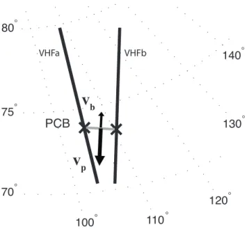
Fig. 2. Schematic presentation of the measurement. The black crosses show the PCB for the two VHF beams and the solid grey line the orientation of the PCB. Vectorsvbandvp are the veloci-ties of the polar cap boundary and plasma along the PCB normal, respectively.
reference polar cap height profile, the ESR 42 m data were averaged to 1 h time resolution. The PCB was determined for the two beams of the VHF separately, which allowed es-timation of the PCB orientation.
The 2-dimensionalE×B plasma drift velocity was
cal-culated from the l-o-s ion velocities of the two VHF radar beams. When doing this, it must be assumed that there are no longitudinal variations in velocity between the beams and that the field-aligned ion velocity is zero. The longitudi-nal separation of the two radar beams increased from 97 to 195 km with latitude. The 2-D velocity vectors were placed in the middle of the gate pairs. For calculating the magnetic field at different latitudes, the IGRF/DGRF-model was used (http://modelweb.gsfc.nasa.gov/models/cgm/cgm.html).
The reconnection electric field was calculated by Eq. (3). A schematic presentation of the situation is shown in Fig. 2. The 2-D plasma velocity as interpolated at the PCB latitude and the components of the plasma velocity (vp) and the PCB
velocity (vb) along the PCB normal were calculated. For
the estimate of the polar cap boundary velocity, 5-min run-ning means at the 1-min resolution of the PCB location were first calculated. These data were further interpolated to 30-s resolution to obtain the PCB velocity estimates at the same time instants as the plasma velocity measurements. It was assumed that the PCB maintains its orientation as it moves in latitude along the magnetic meridian during the one-minute interval, though this condition may not always be true as pointed out by Østgaard et al. (2005).
photons cm-2s-1 2006:18 UT
30
25
20
15
10
5
00 MLT
Fig. 3.UV image taken at 20:06:18 UT on 25 November 2000. The PAE boundary is marked by a white longitudinal arc connecting the white 40-min MLT sector boundaries. The EISCAT PCBs are marked by red crosses (both beams and their average).
2.3 Comparison of EISCAT and Polar UVI data
For the studied interval 17:00–22:00 UT, on 25 November global images of the northern auroral oval were provided by the UV Imager of the Polar satellite (Torr et al., 1995). The UV Imager was taking images with an integration time of 37 s using the LBHl filter (Lyman-Birge-Hopfield long, 160–180 nm). The emission luminosity in the LBHl wave-length band is practically directly proportional to the energy flux of the precipitating electrons. An emission altitude of 120 km is assumed for the LBHl emissions. For the images, only the line of sight correction has been done which takes into account the increased emission when looking through a longer path length of the atmosphere at large angles away from nadir. The dayglow has not been removed since it is northern winter.
The images were collected continuously, excluding short periods at 18:18–18:22 UT, 19:04–19:09 UT and 20:21– 20:25 UT, when the instrument was taking background im-ages. Since the data had a time resolution of 37 s, one com-plete minute time interval could include two or three succes-sive images. Therefore, to compare the UVI data with the EISCAT data, an image sequence of one frame per minute was generated by selecting the image overlapping most with the corresponding one-minute period to represent the time interval.
To estimate the poleward emission boundary PAE, a 40-min wide MLT sector containing both of the VHF radar beams was selected from each image. Then for each sec-tor, a latitude profile of longitudinally averaged emission in-tensities were calculated with a resolution of half a degree in latitude. The latitude profile was interpolated further to a resolution of 0.1◦ and the location of the PAE was
deter-mined by using a ratio value of 0.3 UVmax, where UVmaxis
69 70 71 72 73 74 75 69
70 71 72 73 74 75
VHF PCB aacgmLat (deg)
Polar UVI P
AE aacgmLat (deg)
25 Nov 2000
y = x + a, a = 0.69
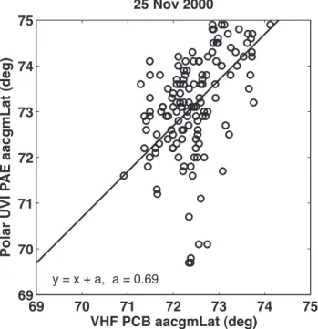
Fig. 4.Comparison of the polar cap boundary estimates by EISCAT VHF and Polar UVI. Linear fit of the formy=x+ahas been applied giving for the constant a-valuea=0.69. The Pearson correlation coefficientr=0.42.
In those cases, a threshold value of 4.3 photons cm−2s−1was used.
Both methods for locating the PAE boundary have been used earlier, in Baker et al. (2000) and Aikio et al. (2006). Baker et al. (2000) found for the Polar UVI images that the optimal ratio and threshold values were 0.3 UVmax and
4.3 cm−2s−1, respectively, when comparing the PAE and the
DMSP b5e boundaries. In addition, when comparing Viking UV with DMSP data, Kauristie et al. (1999) used the ratio value of 0.5 UVmax (full-width half maximum). However,
they stated that the value 1/e∼0.37 could be even better in cases not hampered by background scatter, which is close to the value 0.3 obtained by Baker et al. (2000).
An example of an UVI image taken at 20:06:18 UT is presented in Fig. 3. The calculated PAE latitude (74.7◦) is
marked by a white arc connecting the MLT sector bound-aries. The PCBs from the VHFa (73.7◦), VHFb (73.6◦) and
their average (73.65◦) are marked by red crosses. In this case
the latitudinal difference between the average VHF PCB and PAE was 1.1◦.
In total 138 VHF PCB and UVI PAE pairs could be extracted from the studied substorm time interval 17:00– 22:00 UT. Only those point pairs were included for which both estimates were below 75◦ cgmlat, which is the upper
limit for the EISCAT1Te-method. In addition, the amount of point pairs available was reduced by about an hour data gap in the VHF PCB data between 17:52–18:57 UT (5-min
-6 -4 -2 0 2 4 6
Bx
(
n
T
)
25 Nov 2000 ACE Magnetic field (MAG) Instrument
-6 -4 -2 0 2
By
(
n
T
)
1630 1700 1730 1800 1830 1900 1930 2000 2030 2100 2130 2200 -4
-2 0 2
UT
Bz
(
n
T
)
Fig. 5. IMF components measured in GSM by the ACE satellite (XGSM∼224RE) delayed to the bow shock nose. Vertical line at 18:07 UT indicates the substorm onset time. See details in the text.
running means of the two data sets are visible in Fig. 8). The result is shown as a scatter plot in Fig. 4. Ideally, the points would lie in they=xcurve, but in this event, after making a fit of the formy=x+a, whereais a constant, the UVI PAE appeared to be located typically 0.69◦cgmlat poleward of the
VHF PCB. The Pearson correlation coefficientr calculated for the scatter data set isr=0.42.
We can account a few tenths of a degree of this discrep-ancy to originate from the method used in VHF PCB deter-mination. By default, the PCB is determined as the pole-wardmost latitude where the1Te-curve with errorbars stays above zero, giving somewhat lower latitude values than the curve without errorbars would give (see Aikio et al., 2006). The original latitudinal resolution of the VHF measurements causes at maximum 0.6–0.7◦ uncertainty in the PCB
loca-tion.
Nominally, the field-of-view (f-o-v) resolution of the Polar UV Imager is approximately 0.04◦×0.04◦(Torr et al., 1995)
corresponding typically an ionospheric resolution to 0.3◦
1700 1730 1800 1830 1900 1930 70
71 72 73 74 75 76 77 78
500 m/s
AACGM lat (deg)
UT
2d plasma drift velocity from EISCAT VHF CP4B 25 Nov 2000
1930 2000 2030 2100 2130 2200
70 71 72 73 74 75 76 77 78
500 m/s
AACGM lat (deg)
UT
2d plasma drift velocity from EISCAT VHF CP4B 25 Nov 2000
(a)
(b)
PCB
CRB
00 MLT 00 MLT
00 MLT 00 MLT
00 MLT 00 MLT
00 MLT 00 MLT
00 MLT 00 MLT
30
25
20
15
10
5
30
25
20
15
10
5
30
25
20
15
10
5
30
25
20
15
10
5
30
25
20
15
10
5
photons cm-2s-1
photons cm-2s-1
photons cm-2s-1
photons cm-2s-1
photons cm-2s-1 1837:22 UT
(
a)
(
b)
(
c)
(
d)
(
e)
(
f )
(
g)
(
h)
(
i )
(
j )
1727:26 UT 1809:09 UT
1901:17 UT
1942:22 UT
2100:53 UT
1853:18 UT
1923:22 UT
2003:14 UT
2105:10 UT
3 Substorm on 25 November 2000
3.1 Plasma convection
Figure 5 shows the solar wind IMF measured by the ACE satellite. A dynamic time delay based on a com-bination of minimum variance and cross product phase front normal determination techniques (Weimer et al., 2008a,b, and references therein), has been calculated to take into account the solar wind propagation from the ACE location (XGSM∼224RE) to the Earth’s bow shock nose (XGSM∼14RE) (http://omniweb.gsfc.nasa.gov/form/ sc merge min1.html). The prevailing average solar wind ve-locity was 400 km/s.
During 14:00-18:54 UT the IMFBzcomponent remained mainly weakly southwards, creating favourable conditions for magnetospheric substorms. A northward turning ofBz started at about 18:45 UT andBz remained weakly positive until 20:36 UT except during 19:48–20:29 UT. TheBy com-ponent remained negative practically during the whole pe-riod.
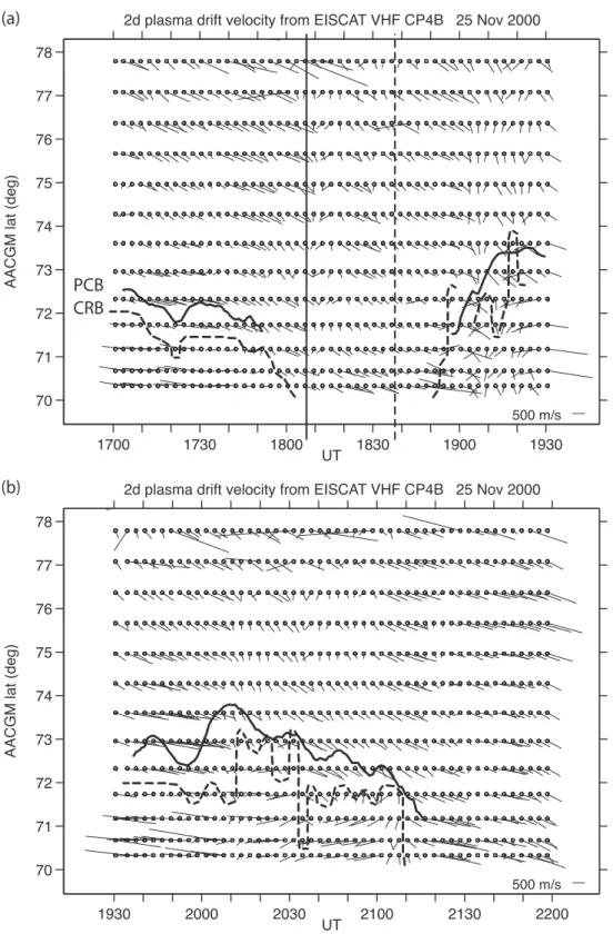
The plasma velocity vectors calculated from the EISCAT VHF data are presented in Fig. 6. The solid black curve is the 5-min running mean of the VHF polar cap boundary at 1-min resolution, and the dashed curve is the plasma convection re-versal boundary (CRB) determined from the plasma velocity vectors. Note that only every third velocity measurement is plotted for the sake of clarity.
The EISCAT measurements started at 17:00 UT and showed a typical evening cell convection pattern with the convection reversal boundary at 72◦
cgmlat. The polar cap boundary was located about 0.5◦ cgmlat poleward of the
CRB. The polar cap boundary moved equatorwards, which is a signature of a substorm growth phase. The CRB fol-lowed closely the motion of the PCB. At 17:52 UT the PCB was abruptly displaced to the south and our method could not see it anymore, and a little bit later also the CRB disappeared from the field of view of the VHF radar.
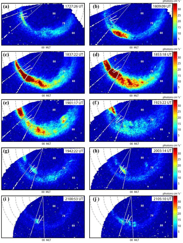
In Fig. 7 a selected set of UVI frames are presented to show the general evolution of the substorm. Most of the frames were selected for reasons that become clear in Sect. 3.5 and may not coincide with the time instants dis-cussed here. Figure 7a was taken during the growth phase of the substorm. The time and location of the substorm on-set was determined from the Polar UVI images. At about 18:07 UT the substorm expansion started around 22:40 MLT by a sudden brightening of aurora on a 40-min wide MLT sector in the equatorward oval (not shown). This was fol-lowed by a magnetic Pi2 pulsation burst at 18:08 UT, de-tected by the SAMNET Borok (Russia) mid-latitude mag-netometer station (54.1◦ cgmlat, 113.3◦ cgmlon, data not
shown). The of the order of 1-min delay between the au-roral signature and the Pi2 burst is consistent with earlier ob-servations of propagation-related delays (Liou et al., 2000).
Here the Borok station was located about 1 h MLT west of the substorm onset region.
Figure 7b shows the situation two minutes after the on-set, when the substorm had expanded poleward and toward west and east. In about 30 min the substorm expansion had progressed so that intense auroral precipitation had intruded into the EISCAT local time from the east (Fig. 7c). At about 18:53 UT the convection reversal boundary reappeared from the south to the EISCAT f-o-v together with the PCB and they both moved polewards (Fig. 6a). During 18:57–19:06 and 19:22–19:31 UT the convection pattern was very dynamic probably violating the assumption of a uniform ion flow be-tween the VHF radar beams. These periods are visible as gaps in the CRB.
The beginning of the recovery phase at about 19:08 UT was determined from the start of the decrease in total in-tegrated westward equivalent current of MIRACLE stations (data not shown). The PCB continued proceeding polewards until 19:23 UT (Fig. 6a and 7f). This is consistent with the observations by Milan et al. (2003), who found that the polar cap area was decreasing due to the poleward contracting PCB in the recovery phase, even after the substorm associated auroral activity had faded away. During the slightly over-lapping gaps in the CRB between 19:22–19:34 UT and in the PCB data between 19:31–19:35 UT, the boundaries had moved equatorwards about half a degree and 0.7 degree, re-spectively. The equatorward motion of the polar cap bound-ary turned poleward at 19:54 UT and lasted until 20:10 UT before turning equatorward again (Fig. 6b). During the stud-ied time interval, the CRB followed the motion of the PCB and was located 0.5-1◦equatorward of the PCB.
3.2 Boundaries and equivalent currents
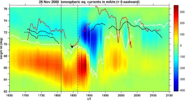
The equivalent currents with the boundaries are shown in Fig. 8. The red curve indicates the 5-min running average of the UVI PAE boundary. The solid and dashed black curves are the VHF PCB and the CRB, respectively. For the sake of clarity, the convection reversal boundary after the onset of the substorm expansion has been left out (see Fig. 6). The white line marks the magnetic convection reversal boundary (MCRB) determined from the equivalent currents. In the premidnight sector until 20:25 UT (∼23:00 MLT), a value of 0 mA/m was used for MCRB. After 20:25 UT, when the westward electrojet was dominating, the −50 mA/m value (corresponding to about −30 nT in the X component) fol-lowed the poleward boundary better.
0
-100
-200
-300
-400 100 200 300
Fig. 8.Equivalent east-west currents calculated from the MIRACLE magnetometer data. Red colour indicates eastward and blue westward flowing electrojet in mA/m (scale on the right). The white line represents the magnetic convection reversal boundary and the Harang discontinuity period is shown by a dashed line. The solid black curve is the PCB by the EISCAT VHF and the red curve is the 5-min running mean of the UVI PAE boundary. The substorm onset at 18:07 UT is marked by a vertical solid line and the expansion to the EISCAT and MIRACLE MLT at 1838 UT by a dashed line. The black triangle at 18:28 UT is the DMSP F15 particle PCB (b5e) measured in the EISCAT MLT sector.
degrees polewards at about 17:21 UT. Similar, though much weaker behaviour can be also seen in the VHF PCB.
At the substorm onset at 18:07 UT, the poleward edge of the EEJ region, followed by the UVI PAE, jumped 2◦cgmlat
equatorwards. The VHF could not see the PCB which was located equatorward of the radar f-o-v, together with the CRB (see also Fig. 6a). After 18:25 UT the EEJ pattern started to move polewards and a few minutes later the UVI PAE fol-lowed. The DMSP F15 satellite was crossing the EISCAT MLT from south to north at 18:28 UT and the particle data of the spacecraft showed a clear poleward particle boundary (b5e) at a latitude 69.6◦(black triangle in Fig. 8), just
equa-torward of the UVI PAE boundary (DMSP data not shown). The b5e boundary represents the poleward edge of the au-roral oval as determined by an abrupt drop in the electron energy flux (Newell et al., 1996a,b).
At 18:36 UT the eastward electrojet started to intensify and the MCRB stopped moving polewards. Two minutes later also the westward electrojet on the poleward side started to intensify. From the Polar UVI images it can be seen that the intensification of the electrojets was associated with the intense auroral activity intrusion from the east to the EIS-CAT/MIRACLE MLT sector (Fig. 7c). The UVI PAE bound-ary continued poleward motion together with the reappearing VHF PCB.
After 18:53 UT the WEJ expanded abruptly by several de-grees to lower latitudes. This was accompanied by fading
away of the most intense precipitation at the EISCAT MLT at 19:01 UT (Fig. 7e). After the Polar UVI data gap 19:04– 19:09 UT the UVI PAE boundary appeared at a very high latitude of about 76◦. However, the emissions were weak
and the intensity latitude profile was flat making the deter-mination of the PAE boundary very uncertain. In addition, the wobble of the Polar satellite may have stretched the au-roral forms polewards. The VHF PCB remained below 74◦
cgmlat.
After about 19:13 UT, the eastward electrojet recovered, first at latitudes below 67◦, in association with the weakening
of the WEJ. From ∼19:27 UT onwards the equivalent cur-rent pattern was again dominated by the eastward electrojet, although with a lower intensity level. The westward electro-jet intensified for a short period at 20:05 UT, associated with a poleward excursion of the PCB. After 20:22 UT the WEJ appeared in the post-midnight sector and the UVI PAE and the VHF PCB together followed closely the poleward edge of the westward electrojet.
3.3 Harang discontinuity
After 18:38 UT an intense westward electrojet formed on the poleward side of the intensifying eastward electrojet. The WEJ expanded from the east, probably rotating the whole current pattern to an earlier MLT. By 19:00 UT the WEJ re-gion had expanded equatorward down to latitudes 65◦
the MIRACLE magnetometer stations showed a change from positive to negative X, which is the original definition of the Harang discontinuity near magnetic midnight (Heppner, 1972). This MCRB is shown by a white dashed line in Fig. 8. Within the HD region, both of the electrojets had periodic, about 3-min fluctuations, whose effect can be seen in oscilla-tory motion of the MCRB. After 19:13 UT the MCRB moved poleward and the electrojets weakened, while the most in-tense auroral activity had already faded in this MLT sector. The dynamic convection pattern after 19:22 UT was associ-ated with the recovery of the EEJ.
Amm et al. (2000) distinguished two topologically differ-ent type of HD, ”rotation-type” and ”expansion-type”, the former being associated with the Earth’s rotation and ob-served during quiet and moderately active geomagnetic con-ditions without substorm activity, and the latter during ge-omagnetically disturbed periods i.e. during substorms, typi-cally appearing in an earlier MLT sector. The Harang discon-tinuity period in this event represents the ”expansion-type” HD.
When the WEJ associated with the Harang discontinuity intruded from the east to the EISCAT MLT sector, the UVI PAE and the VHF PCB moved rapidly in the poleward di-rection. Still, a part of the WEJ was flowing poleward of the polar cap boundary proxies (Fig. 8). Only after about 19:10 UT almost all of the WEJ was located equatorward of these boundaries.
Figure 8 indicates that, in the Harang discontinuity region, the poleward part of the westward equivalent electrojet was flowing poleward of the UVI PAE and the VHF polar cap boundaries. Equivalent currents are the part of the real three-dimensional current system that are visible to the ground. The real east-west currents are likely to deviate to some ex-tent from the equivalent east-west currents. The MIRACLE magnetometer Y components showed positive disturbances with quasi-periodic variations of a few minutes up to 71.5◦
cgmlat between 18:30 and 19:00 UT (data not shown). At the same time, Polar UVI images showed structured precip-itation within the auroral bulge. Hence, it is plausible that structured upward field-aligned currents were flowing from this region. In addition, there is a gap in latitudinal cover-age of magnetometer stations between BJN (71.5◦cgmlat)
and HOR (74.1◦ cgmlat), which decreases the accuracy of
the 1-D upward continuation method within the region of in-terest. Because of these uncertainties, more investigations within the expansion type HD should be made to verify the extension of the WEJ to the polar cap.
3.4 Reconnection electric field
The results of the calculated ionospheric reconnection elec-tric field are presented in the three topmost panel in Fig. 9. The topmost panel shows the plasma drift velocity along the PCB normal, positive equatorwards. The second panel shows
the same velocity component for the PCB motion. The third panel presents the calculated reconnection electric fieldEr.
During the substorm growth phase, before 18:07 UT, dur-ing polar cap expansion,Ervaried between 0–10 mV/m. The magnitudes are in agreement with earlies studies, e.g. de la Beaujardiere et al. (1991) found thatEris less than 15 mV/m when the polar cap expands and Blanchard et al. (1997) ob-tained values less than 10 mV/m before a substorm onset.
Because the PCB was located equatorward of the radar measurement range, the reconnection electric field could not be calculated during the substorm onset and early expan-sion. In the late expansion and the recovery phasesEr var-ied between 15 and 40 mV/m, which are of the same order of magnitude as found in earlier studies (de la Beaujardiere et al., 1991; Blanchard et al., 1997; Østgaard et al., 2005). The electric field showed also variations with periods of∼7– 27 min. These variations are interpreted as variable recon-nection occuring in the magnetotail and have been reported in earlier studies (e.g. Østgaard et al., 2005; Aikio et al., 2008). 3.5 Reconnection electric field and auroral emissions
In this section, the variations in the reconnection electric field are compared to the optical auroral emissions by the Polar UVI instrument.
For a comparison with the reconnection electric field, a weighted emission intensity average was calculated for UVI images corresponding to EISCAT data points (1 min resolu-tion, bottom panel in Fig. 9). The calculation was made from a 80-min wide MLT sector including the EISCAT beams with latitude limits of 65◦and 80◦cgmlat. The emission
intensi-ties within the MLT sector were averaged in longitude by using 0.5◦-wide latitude bins. The final result was obtained
by weighting these longitudinal averages with their area and calculating the average. The 40-min wide MLT sector was enlargened to 80-min wide sector due to that also possible auroral emission intensifications occuring close to the EIS-CAT but not exactly at the radar beams, would be included in the calculation.
During the growth phaseEr intensified around 17:25 UT (line a in Fig. 9). Polar UVI showed the formation of an east-west oriented auroral arc at the poleward edge of the oval in the evening sector within the f-o-v of EISCAT (Fig. 7a). The structure was 3 MLT hours wide and lasted about 12 min from 17:26 UT to 17:38 UT. The brightening of the arc could be seen as an intensification of Polar UVI intensity (bottom panel of Fig. 9) The IMFBzhad been mainly weakly south-wards for several hours loading the magnetosphere (Fig. 5). This weak reconnection burst with associated localized au-roral activation is a signature of release of a small amount of the energy stored into the magnetotail before the actual substorm about 40 min later at 18:07 UT.
0 200 400 600
Vp
la
sm
a
[m/s]
-600 -400 -200 0 200 400
Vb
o
u
n
d
a
ry
[m/s]
-10 0 10 20 30 40
Er
[mVm
-1]
17 18 19 20 21
3 4 5 6 7 8 9 10
UVI intensity [photons cm
-2s -1]
equatorwards
polewards
equatorwards
polewards
a a
a
f
f g
g
g h
h
h
i
i
i
UT
Fig. 9. Plasma drift velocity along the PCB normal, positive equatorwards (top panel). PCB velocity along the PCB normal, positive equatorwards (2nd panel). Ionospheric reconnection electric field, positive values indicate magnetic flux closure in the magnetotail (3rd panel). Vertical dotted lines show the maxima of theEr associated with auroral PBIs. The corresponding UVI frames in Fig. 9 are shown by a letter. Weighted average UV intensity (bottom panel).
18:58–19:17 UT were associated with rapid fading of bright aurora in the EISCAT local time sector at 19:00–19:03 UT while the most intense precipitation concentrated about an hour MLT westward of EISCAT (Fig. 7e).
The activation is obviously an auroral poleward bound-ary intensification (PBI) at the poleward boundbound-ary of the oval. PBIs are transient nightside geomagnetic disturbances with a localized auroral signature that appear at the poleward boundary of the auroral oval and can then extend equator-ward inside the auroral oval (Lyons et al., 1999; Zesta et al., 2002). PBIs occur during all levels of geomagnetic activity (Lyons et al., 1998).
The intensification ofEr which maximized at 19:41 UT (line g in Fig. 9) was associated with a localized poleward boundary intensification at the poleward boundary of the
double oval (Elphinstone et al., 1995) in the EISCAT MLT sector (Fig. 7g). The UVI intensity curve showed a peak close to the Er maximum. The IMFBz had a southward excursion during the preceeding 15 min (Fig. 5). The PBI was about 1.5 h MLT wide and lasted roughly 8 min, 19:41– 19:49 UT.
The nextEr maximum, which was also associated with a PBI, occured at 20:01 UT (line h in Fig. 9). The PBI was localized within about the same 1.5 h–wide MLT range as the previous PBI. The PBI lasted about 9 min, from 20:01 to 20:10 UT. BothEr and the averaged UVI intensity showed a very clear peak.
PBI in Fig. 7i is not known, but the activation started before 21:01 UT and ended at about 21:10 UT. The width of the PBI was about 0.5 h MLT in the beginning, but it evolved quickly to multiple beads extending over 3 h MLT (Fig. 7j). During the maximumEr, UVI had a data gap, but a maximum in the averaged intensity was observed about 5 min later.
From the second panel of Fig. 9 it can be seen that all of the enhancements inEr were associated with a poleward con-tracting polar cap boundary. The main factor in producing the calculated reconnection electric field was the poleward motion of the PCB in events a, h and i. The enhancement in equatorward plasma flow was mainly responsible for re-connection electric field in events f and g (Fig. 9, top panel). The latter case is in accordance with de la Beaujardiere et al. (1994) who observed that the flow rate across the pole-ward boundary of the aurora was increased significantly dur-ing the periods of PBIs. De la Beaujardiere et al. concluded that the feature is associated with a local increase in the re-connection rate (in accordance with the Eq. 3) with qualita-tively estimated peak values of the order of 25 mV/m.
Besides the PBIs in the 80-min wide MLT sector cen-tered at EISCAT that are described above, PBIs occurred also in other MLT sectors. In the growth phase, several east-west oriented PBIs appeared, typically between 21:00 and 22:00 MLT. The brightenings were about 2 MLT wide and lasted from 3 min to 15 min. In the recovery phase, a few additional PBIs could be distinguished.
4 Summary and discussion
We have studied some specific aspects of the reconnection process that can be related to high-latitude boundaries. The dynamics of the polar cap boundary in the evening sector during a substorm on 25 November 2000 were examined by using EISCAT incoherent scatter radar measurements. As a measure of the nightside reconnection rate, the local ionospheric reconnection electric field was estimated by the method introduced by Vasyliunas (1984), where the elec-tric field is calculated by using plasma flow across the PCB. The plasma drift velocity was calculated from the dual-beam measurements of the EISCAT VHF radar, and the PCB was determined using EISCAT measurements on both the main-land and Svalbard by using the method by Aikio et al. (2006). The VHF PCB was compared with the poleward auro-ral emission boundary extracted from global optical images of the Polar UV Imager. On the average, the PAE bound-ary was located 0.7◦
poleward of the EISCAT PCB in this event, though large scatter occured in individual points. The most probable cause for the difference in the UVI PAE and the VHF PCB locations is the wobble of the Polar satel-lite, which causes smearing of UVI images along the wob-ble direction. In this case, the wobbling was unfortunately in the direction in which the PAE boundary was determined (∼10:00–22:00 MLT). During one DMSP overflight, a close
co-location of the b5e boundary (poleward edge of the oval) and the PAE boundary was found (the PCB was at too low a latitude at that moment for the EISCAT VHF to see it).
The calculation of the 2-D plasma velocity vectors allowed the determination of the convection reversal boundary from the EISCAT data. A striking feature was the similar tempo-ral evolution of the PCB (fromTe data) and the CRB (from plasma velocity data), lending credence for the method of PCB determination. The CRB was observed to follow the motion of the PCB and to be located 0.5–1◦ cgmlat
equa-torward of the PCB. The offset is consistent with the results by Sotirelis et al. (2005), who compared SuperDARN HF radar boundaries with DMSP particle boundaries. Sotirelis et al. found an equatorward offset of the CRB relative to the PCB that varies according to the local time from zero near noon to ∼1◦ near dawn and dusk and is largest near
mid-night. In the early morning sector, offset as large as 3–4◦
has been observed (Amm et al., 2003). The PCB-CRB offset is interpreted to result from a small viscous-like interaction between the magnetosheath and the low-latitude boundary layer, resulting in antisunward flow on closed field lines next to the polar cap boundary (Sotirelis et al., 2005, and refer-ences therein).
The VHF PCB, the CRB, and the UVI PAE boundary were studied in a framework of the 1-D ionospheric equivalent east-west electrojets calculated from the MIRACLE mag-netometer measurements by using the upward continuation method by Vanham¨aki et al. (2003). During the substorm growth phase, all the boundaries showed a similar drift mo-tion equatorwards on the poleward side of the eastward elec-trojet region. The UVI PAE boundary was generally located poleward of the VHF PCB with varying distances.
The onset of the substorm expansion occured about 2 h MLT east of the observed local time sector and was as-sociated with a sudden equatorward leap of 2◦ of the EEJ
region. After 31 min a dynamical electrojet pattern was ob-served to expand to the EISCAT MLT in association with intense auroral activity. The current pattern was formed by intense westward electrojet on the poleward side of the east-ward electrojet and was in the f-o-v of EISCAT and MIR-ACLE for about 50 min. We interpret the current system to represent a dynamical ”expansion-type” Harang discontinu-ity, after classification by Amm et al. (2000). Within the Ha-rang discontinuity region, the UVI PAE and the VHF PCB boundaries moved rapidly poleward within the WEJ. A part of the calculated equivalent westward electrojet was flowing poleward of the boundaries.
Later in the recovery phase, the boundaries generally moved equatorwards. After shifting to the post-midnight sector, the VHF PCB and the UVI PAE followed together the poleward edge of the WEJ. The separation of the CRB and the MCRB in the growth and the recovery phases is con-sistent with earlier evening sector studies where the MCRB was found to be typically located 1–2◦cgmlat equatorward
the post-midnight sector the MCRB was found to be located 1–2◦ poleward of the CRB, which is close to the values of
0.5–1◦
observed earlier by Amm et al. (2003). It is suggested that the shift is due to the field-aligned currents flowing in the vicinity of the HD (Amm, 1998; Amm et al., 2003).
The calculated local ionospheric reconnection electric field was found to vary between 0 and 10 mV/m during the substorm growth phase. During the late expansion and recov-ery phases, values up to 40 mV/m were observed. The val-ues are in agreement with earlier studies (de la Beaujardiere et al., 1991; Blanchard et al., 1997; Østgaard et al., 2005). During the latter period, the electric field showed also varia-tions with periods of∼7–27 min. Similar periods have been reported in previous studies and interpreted as variable re-connection occuring in the magnetotail (e.g. Østgaard et al., 2005; Aikio et al., 2008).
Comparison of the reconnection electric field with the Polar UVI data showed a clear correlation between inten-sifications of Er and auroral poleward boundary intensi-fications (PBIs). The PBIs appeared within one minute of the ionospheric reconnection electric field maxima and lasted 5–12 min. The PBI-associated Er maxima values were 12 mV/m in the growth phase and 27 mV/m, 32 mV/m, 27 mV/m and 26 mV/m in the recovery phase. The widths of the PBIs were 3 h MLT in the growth phase and 1.5 h MLT in the recovery phase. For the last PBI in the late recov-ery/quiet phase the width was initially 0.5 h MLT but then the PBI evolved into beads covering about 3 h MLT.
In all the five cases, the PCB contracted poleward, but in two cases during the substorm recovery phase, enhanced plasma flow velocity equatorward, across the PCB, was the main factor in producing the enhanced reconnection electric field. An enhanced southward plasma velocity in association with arc intensifications at the poleward auroral boundary have been observed also by de la Beaujardiere et al. (1994).
It has been suggested that when the UVI intensity is high, there is a high ionospheric conductivity and significant fric-tional coupling between the ionospheric plasma and the neu-tral atmosphere. Then plasma flows are retarded and it is the PCB that moves. When the conductivity is low, iono-spheric flows are excited rather than motions of the PCB (Boudouridis et al., 2008). In this study, the PCB motions were generally associated with bright emissions at the bound-ary and thus with high conductivities. However, the largest plasma flow in event g was also associated with rather intense emissions, in contradiction with Boudouridis et al. (2008). The other plasma flow event f was indeed associated with less intense emissions at the boundary. To make clear con-clusions, more events should be studied.
PBIs are generally considered as ionospheric signatures of longitudinally narrow earthward plasma sheet flow bursts, bursty bulk flows (BBFs) (Lyons et al., 2002, and refer-ences therein). For the source of PBIs and BBFs, two pro-cesses have been suggested: localized distant X line recon-nection bursts (Sergeev et al., 2000) and global ULF
pulsa-tion modes of the magnetosphere (Lyons et al., 2002). Zesta et al. (2002) found the PBIs are either equatorward extend-ing (N-S or E-W structures) or non-equatorward extendextend-ing. They suggested that the equatorward extending north-south PBIs would be associated with longitudinally narrow BBFs whereas the wider east-west oriented structures could be as-sociated with the global ULF modes. The non-equatorward extending PBI structures would be associated with a shear in-stability at the separatrix boundary. However, recently Zesta et al. (2006) deduced that every equatorward extending PBI structure they studied, including both north-south and east-west structures, was associated with a fast flow channel in the tail within the same local time sector.
Aikio et al. (2008) found periodic poleward expansions of the PCB which were associated with intensifications of the WEJ in the vicinity of the PCB in a recovery phase of a substorm. Since no signatures of global ULF waves were found, they suggested that enhanced reconnection bursts took place in the tail. In this study, at least one clear localized WEJ enhancement with a simultaneous poleward expanding PCB was observed after 20:00 UT, and by utilizing the dual-beam VHF measurements we were able to show that it indeed was associated with an enhanced reconnection electric field (line h in Fig. 9).
The spatial resolution of the Polar UV Imager was not high enough in this case to tell whether or not the PBIs were nar-row auroral structures that propagated equatorward. How-ever, they all, including the last one with multiple beads, were associated with enhanced reconnection, which suggests that the PBIs were a consequence of temporarily enhanced longitudinally localized magnetic flux closure in the magne-totail.
Acknowledgements. The authors are grateful to Ritva Kuula for help in the EISCAT data analysis. The EISCAT is an interna-tional association supported by research organisations in China (CRIRP), Finland (SA), France (CNRS, till end 2006), Germany (DFG), Japan (NIPR and STEL), Norway (NFR), Sweden (VR), and the United Kingdom (STFC). The authors thank George Parks and Matt Fillingim for the Polar UVI data, and N. Ness, CDAWEB and SPDF/OMNIWeb for the ACE data and the SPDF/Modelweb for IGRF/DGRF-model parameters. The MIRACLE network is operated as an international collaboration under the leadership of the Finnish Meteorological Institute. The DMSP particle detectors were designed by Dave Hardy of AFRL, and data obtained from JHU/APL. We thank D. Hardy, F. Rich, and P. Newell for its use. The Sub-Auroral Magnetometer Network data (SAMNET) is oper-ated by the Department of Communications Systems at Lancaster University (UK) and is funded by the Science and Technology Fa-cilities Council (STFC). The work by AK has been supported by the Academy of Finland (project 115920).
References
Aikio, A. T., Pitk¨anen, T., Kozlovsky, A., and Amm, O.: Method to locate the polar cap boundary in the nightside ionosphere and application to a substorm event, Ann. Geophys., 24, 1905–1917, 2006, http://www.ann-geophys.net/24/1905/2006/.
Aikio, A. T., Pitk¨anen, T., Fontaine, D., Dandouras, I., Amm, O., Kozlovsky, A., Vaivdas, A., and Fazakerley, A.: EISCAT and Cluster observations in the vicinity of the dynamical polar cap boundary, Ann. Geophys., 26, 87–105, 2008,
http://www.ann-geophys.net/26/87/2008/.
Amm, O.: Method of characteristics in spherical geometry applied to a Harang-discontinuity situation, Ann. Geophys., 16, 413– 424, 1998, http://www.ann-geophys.net/16/413/1998/.
Amm, O., Janhunen, P., Opgenoorth, H. J., Pulkkinen, T. I., and Viljanen, A.: Ionospheric shear flow situations observed by the MIRACLE network, and the concept of Harang Discontinuity, AGU monograph on magnetospheric current systems, Geophys-ical Monograph, 118, 227–236, 2000.
Amm, O., Aikio, A., Bosqued, J.-M., Dunlop, M., Fazakerley, A., Janhunen, P., Kauristie, K., Lester, M., Sillanp¨a¨a, I., Tay-lor, M. G. G. T., Vontrat-Reberac, A., Mursula, K., and Andr´e, M.: Mesoscale structure of a morning sector ionospheric shear flow region determined by conjugate Cluster II and MIRACLE ground-based observations, Ann. Geophys., 21, 1737–1751, 2003, http://www.ann-geophys.net/21/1737/2003/.
Baker, J. B., Clauer, C. R., Ridley, A. J., Papitashvili, V. O., Brit-tnacher, M. J., and Newell, P. T.: The nightside poleward bound-ary of the auroral oval as seen by DMSP and the ultraviolet im-ager, J. Geophys. Res., 105, 21267–21280, 2000.
Baker, K. and Wing, S.: A new magnetic coordinate system for conjugate studies at high latitudes, J. Geophys. Res., 94 , 9139– 9143, 1989.
de la Beaujardiere, O., Lyons, L.R., and Friis-Christensen, E.: Son-drestrom radar measurements of the reconnection electric field, J. Geophys. Res., 96, 13907–13912, 1991.
de la Beaujardiere, O., Lyons, L.R., Ruohoniemi, J. M., Friis-Christensen, E., Danielsen, C., Rich, F. J., and Newell, P. T.: Quiet-time intensifications along the poleward auroral boundary near midnight, J. Geophys. Res., 99, 287–298, 1994.
Blanchard, G. T., Lyons, L. R., de la Beaujardiere, O., Doe, R. A., and Mendillo, M.: Measurement of the magnetotail reconnection rate, J. Geophys. Res., 101, 15265–15276, 1996.
Blanchard, G. T., Lyons, L. R., and de la Beaujardiere, O.: Mag-netotail reconnection rate during magnetospheric substorms, J. Geophys. Res., 102, 24303–24312, 1997.
Boudouridis, A., Lyons, L. R., Zesta, E., Ruohoniemi, J. M., and Lummerzheim, D.: Nightside flow enhancement associated with solar wind dynamic pressure driven reconnection, J. Geophys. Res., 113, A12211, doi:10.1029/2008JA013489, 2008.
Cowley, S. W. H: Magnetosphere-ionosphere interactions: a tutorial review, AGU monograph on magnetospheric current systems, Geophysical Monograph, 118, 91–106, 2000.
Cowley, S. W. H. and Lockwood, M.: Excitation and decay of so-lar wind-driven flows in the magnetosphere-ionosphere system, Ann. Geophys., 10, 103–115, 1992.
Dungey, J. W.: Interplanetary field and the auroral zones, Phys. Res. Lett., 6, 47-48, 1961.
Elphinstone, R. D., Hearn, D. J., Cogger, L. L., et al.: The double oval auroral distribution, 2., The most poleward arc system and
the dynamics of the magnetotail, J. Geophys. Res., 100, 12093– 12102, 1995.
Fontaine, D. and Peymirat, C.: Large-scale distributions of iono-spheric horizontal and field-aligned currents inferred from EIS-CAT, Ann. Geophys., 14, 1284–1296, 1996,
http://www.ann-geophys.net/14/1284/1996/.
Heppner, J. P.: The Harang discontinuity in auroral belt ionospheric currents, Geophys. Norv., 29, 105–120, 1972.
Hubert, B., Milan, S. E., Grocott, A., Blockx, C., Cowley, S. W. H., and G´erard, J.-C.: Dayside and nightside recon-nection rates inferred from IMAGE FUV and Super Dual Auroral Radar Network, J. Geophys. Res., 111, A03217, doi:10.1029/2005JA011140, 2006.
Kauristie, K., Weygand, J., Pulkkinen, T.I., Murphree, J. S., and Newell, P. T.: Size of the auroral oval: UV ovals and precipitation boundaries compared, J. Geophys. Res., 104, 2321–2331, 1999. Koskinen, H. E. J. and Pulkkinen, T. I.: Midnight velocity shear
zone and the concept of Harang discontinuity, J. Geophys. Res., 100, 9539–9547, 1995.
Liou, K., Meng, C.-I, Newell, P. T., Takahashi, K., Ohtani, S.-I., Lui, A. T. Y., Brittnacher, M., and Parks, G.: Evaluation of low-latitude Pi2 pulsations as indicators of substorm onset using Po-lar ultraviolet imagery, J. Geophys. Res., 105, 2495–2505, 2000. Lyons, L. R., Blanchard, G. T., Samson, J. C., Ruohoniemi, J. M., Greenwald, R. A., Reeves, G. D., and Scudder, J. D.: Near Earth plasma sheet penetration and geomagnetic disturbances, AGU monograph on new perspectives on the Earth’s magnetotail, Geo-physical Monograph, 105, 241–257, 1998.
Lyons, L. R., Nagai, T., Blanchard, G. T., Samson, J. C., Yamamoto, T., Mukai, T., Nishida, A., and Kokubun, S.: Association be-tween Geotail plasma flows and auroral poleward boundary in-tensifications observed by CANOPUS photometers, J. Geophys. Res., 104, 4485–4500, 1999.
Lyons, L. R., Zesta, E., Xu, Y., Sanchez, E. R., Samson, J. C., Reeves, G. D., Ruohoniemi, J. M., and Sigwarth, J. B.: Auro-ral poleward boundary intensifications and tail bursty flows: A manifestation of a large-scale ULF oscillation, J. Geophys. Res., 107, 1352, doi:10.1029/2001JA000242, 2002.
Milan, S. E., Lester, M., Cowley, S. W. H., Oksavik, K., Brittnacher, M., Greenwald, R. A., Sofko, G., and Villain, J.-P.: Variations in the polar cap area during two substorm cycles, Ann. Geophys., 21, 1121–1140, 2003,
http://www.ann-geophys.net/21/1121/2003/.
Milan, S. E.: Dayside and nightside contributions to the cross polar cap potential: placing an upper limit on a viscous-like interac-tion, Ann. Geophys., 22, 3771–3777, 2004,
http://www.ann-geophys.net/22/3771/2004/.
Newell, P. T., Feldstein, Y. I., Galperin, Y. I., and Meng, C.-I.: Morphology of nightside precipitation, J. Geophys. Res., 101, 10737–10748, 1996a.
Newell, P. T., Feldstein, Y. I., Galperin, Y. I., and Meng, C.-I.: Cor-rection to ”Morphology of nightside precipitation” by Patrick T. Newell, Yasha I. Feldstein, Yuri I. Galperin,and Ching-I. Meng, J. Geophys. Res., 101, 17419–17421, 1996b.
Østgaard, N., Moen, J., Mende, S. B., Frey, H. U., Immel, T. J., Gal-lop, P., Oksavik, K., and Fujimoto, M.: Estimates of magnetotail reconnection rate based on IMAGE FUV and EISCAT measure-ments, Ann. Geophys., 23, 123–134, 2005,
Parks, G., Brittnacher, M., Chen, L. J., Elsen, R., McCarthy, M., Germany, G., and Spann, J.: Does the UVI on Polar detect cos-mic snowballs, Geophys. Res. Lett., 24, 3109–3112, 1997. Senior, C., Delcourt, D., Cerisier, C., Hanuise, C., Villain,
J.-P., Greenwald, R. G., Newell, P. T., and Rich, F. J.: Correlated observations of the boundary between polar cap and nightside auroral zone by HF radars and the DMSP satellite, Geophys. Res. Lett., 21, 221–224, 1994.
Sergeev, V. A.: Multiple-spacecraft observation of a narrow tran-sient plasma jet in the Earths plasma sheet, Geophys. Res. Lett., 27, 851–854, 2000.
Siscoe, G. L. and Huang T. S.: Polar cap inflation and deflation, J. Geophys. Res., 90, 543–547, 1985.
Sotirelis, T., Ruohoniemi, J. M., Barnes, R. J., Newell, P. T., Greenwald, R. A., Skura, J. P., and Meng, C.-I.: Com-parison of SuperDARN radar boundaries with DMSP parti-cle precipitation boundaries, J. Geophys. Res., 110, A06302, doi:10.1029/2004JA010732, 2005.
Tanaka, T.: Configuration of the magnetosphere-ionosphere con-vection system under northward IMF conditions with nonzero IMFBy, J. Geophys. Res., 104, 14683–14690, 1999.
Torr, M., Torr, D. G., Zukic, M., Johnson, R. B., Ajello, J., Banks, P., Clark, K., Cole, K., Keffer, C., Parks, G., Tsurutani, B., and Spann, J.: A far ultraviolet imager for the International Solar-Terrestrial Physics Mission, Space Sci. Rev., 71, 329–383, 1995.
Vanham¨aki, H., Amm, O., and Viljanen, A.: 1-dimensional up-ward continuation of the ground magnetic field disturbance us-ing spherical elementary current systems, Earth Planets Space, 55, 613–625, 2003.
Vasyliunas, V. M.: Steady state aspects of magnetic field line merg-ing, AGU monograph on magnetic reconnection in space and lab-oratory plasmas, Geophysical Monograph, 30, 25–31, 1984. Weimer, D. R. and King, J. H.: Improved calculations of
interplanetary magnetic field phase front angles and prop-agation time delays, J. Geophys. Res., 113, A01105, doi:10.1029/2007JA012452., 2008a.
Weimer, D. R. and King, J. H.: Correction to ”Improved cal-culations of interplanetary magnetic field phase front angles and propagation time delays”, J. Geophys. Res., 113, A07106, doi:10.1029/2008JA013075., 2008b.
Zesta, E., Donovan, E., Lyons, L., Enno, G., Murphree, J. S., and Cogger, L.: Two-dimensional structure of auroral poleward boundary intensifications, J. Geophys. Res., 107, 1350–1369, doi:10.1029/2001JA000260, 2002.