Measurements of the Microbial Unknown
Manuel E. Lladser1*, Rau´l Gouet2, Jens Reeder3
1Department of Applied Mathematics, University of Colorado, Boulder, Colorado, United States of America,2Centro de Modelamiento Matema´tico (CNRS UMI 2807), Universidad de Chile, Santiago, Chile,3Department of Chemistry and Biochemistry, University of Colorado, Boulder, Colorado, United States of America
Abstract
The availability of high-throughput parallel methods for sequencing microbial communities is increasing our knowledge of the microbial world at an unprecedented rate. Though most attention has focused on determining lower-bounds on the a-diversity i.e. the total number of different species present in the environment, tight bounds on this quantity may be highly uncertain because a small fraction of the environment could be composed of a vast number of different species. To better assess what remains unknown, we propose instead to predict the fraction of the environment that belongs to unsampled classes. Modeling samples as draws with replacement of colored balls from an urn with an unknown composition, and under the sole assumption that there are still undiscovered species, we show that conditionally unbiased predictors and exact prediction intervals (of constant length in logarithmic scale) are possible for the fraction of the environment that belongs to unsampled classes. Our predictions are based on a Poissonization argument, which we have implemented in what we call the Embedding algorithm. In fixed i.e. non-randomized sample sizes, the algorithm leads to very accurate predictions on a sub-sample of the original sample. We quantify the effect of fixed sample sizes on our prediction intervals and test our methods and others found in the literature against simulated environments, which we devise taking into account datasets from a human-gut and -hand microbiota. Our methodology applies to any dataset that can be conceptualized as a sample with replacement from an urn. In particular, it could be applied, for example, to quantify the proportion of all the unseen solutions to a binding site problem in a random RNA pool, or to reassess the surveillance of a certain terrorist group, predicting the conditional probability that it deploys a new tactic in a next attack.
Citation:Lladser ME, Gouet R, Reeder J (2011) Extrapolation of Urn Models via Poissonization: Accurate Measurements of the Microbial Unknown. PLoS ONE 6(6): e21105. doi:10.1371/journal.pone.0021105
Editor:Dongxiao Zhu, University of New Orleans, United States of America ReceivedFebruary 15, 2011;AcceptedMay 19, 2011;PublishedJune 28, 2011
This is an open-access article, free of all copyright, and may be freely reproduced, distributed, transmitted, modified, built upon, or otherwise used by anyone for any lawful purpose. The work is made available under the Creative Commons CC0 public domain dedication.
Funding:M. Lladser was partially supported by NASA ROSES NNX08AP60G and NIH R01 HG004872. R. Gouet was supported by FONDAP, BASAL-CMM and Fondecyt 1090216. J. Reeder was supported by a post-doctoral scholarship from the German Academic Exchange Service (DAAD). M. Lladser and R. Gouet are thankful to the project Nu´cleo Milenio Informacio´n y Aleatoriedad, which facilitated a research visit to collaborate in person. The funders had no role in study design, data collection and analysis, decision to publish, or preparation of the manuscript.
Competing Interests:The authors have declared that no competing interests exist. * E-mail: [email protected]
Introduction
A fundamental problem in microbial ecology is the ‘‘rare biosphere’’ [1] i.e. the vast number of low-abundance species in any sample. However, because most species in a given sample are rare, estimating their total number i.e.a-diversity is a difficult task [2,3], and of dubious utility [4,5]. Although parametric and non-parametric methods for species estimation show some pro-mise [6,7], microbial communities may not yet have been sufficiently deeply sampled [8] to test the suitability of the models or fit their parameters. For instance, human-skin communities demonstrate an unprecedented diversity within and across skin locations of same individuals, with marked differences between specimens [9].
In an environment composed of various but an unknown number of species, letpi§0be the proportion in which a certain species i occurs. Samples from microbial communities may be conceptualized as sampling–with replacement–different colored balls from an urn. The urn represents the environment where samples are taken: soil, gut, skin, etc. The balls represent the different members of the microbial community, and each color is a uniquely defined operational taxonomic unit.
In the non-parametric setting, the urn is composed by an unknown number of colors occurring in unknown relative proportions. In this setting, the a-diversity of the urn [10] corresponds to the cardinality of the set fi:piw0g. Although various lower-confidence bounds for this parameter have been proposed in the literature [11–14], tight lower-bounds on a-diversity are difficult in the non-parametric setting because a small fraction of the urn could be composed by a vast number of different colors [15]. Motivated by this, we shift our interest to predicting instead the fraction of balls with a color unrepresented in the firstnobservations from the urn. This is the unobservable random variable:
Un~ X
i[=fX1,...,Xng
pi~1{ X i[fX1,...,Xng
pi,
observation is preciselyUn, and the mean number of additional observations to discover a new color is 1=Un. We note that (1{Un)corresponds to what is called the conditional coverage of a sample of sizenin the literature. For this reason, we refer toUn as theconditional uncovered probabilityof the sample.
The expected value ofUnis given by:
un~ (Un)~X i
pi(1{pi)n:
Unlike the conditional uncovered probability of the sample,unis a parameter that depends on the unknown urn composition but not on the specific colors observed in the sample. Interest in the above quantities or related ones has ranged from estimating the probability distribution of the keys used in the Kenngruppenbuch
(the Enigma cipher book) in World War II [16], to assessing the confidence that an iterative procedure with a random start has found the global maximum of a given function [17], to predicting the probability of discovering a new gene by sequencing additional clones from a cDNA library [18]. We note that(1{un)is called theexpected coverage of the samplein the literature.
Various predictors of Un and estimators of un have been proposed in the literature. These are mostly based on a user-defined parameterr§0and the statisticsN(k,nzr),k~0,. . .,r; defined as the number of colors observed k-times, when r additional balls are sampled from the urn.
Turing and Good [19] proposed to estimateunusing the biased statistic vn,0~N(1,n)=n. Posteriorly, Robbins [20] proposed to predictUnusing
vn,1~
N(1,nz1)
(nz1) , ð1Þ
which he showed to be unbiased forunand to satisfy the inequality f(Un{vn,1)2gv1=(nz1). Despite the possibly small quadratic variation distance between Un and Robbins’ estimator, and as illustrated by the plots on the left side of Fig. 1, when using Robbins’ estimator to predictUnsequentially withn(to assess the quality of the predictions at various depths in the sample), we observe that unusually small or large values of N(1,nz1) may offset subsequent predictions ofUn. In fact, as seen on the right-hand plots of the same figure, an offset prediction is usually followed by another offset prediction of the same order of magnitude, even100observations later (correlation coefficient of green clouds, R~0:934991 and R~0:948600 on top- and bottom-right plots).
Subsequently, for eachr§1, Starr [21] proposed to predictUn using
vn,r~ Xr
k~1 r{1
k{1
nzr k
:N(k,nzr): ð2Þ
Even thoughvn,ris the minimum variance unbiased estimator of un based on r additional observations from the urn [22], Starr showed that vn,r may be strongly negatively correlated with Un whenr~1(note that Starr’s and Robbins’ estimators are identical when r~1). Furthermore, the sequential prediction of Un via Starr’s estimator is affected by issues similar to Robbins’ estimator, which is also illustrated in Fig. 1, even when the parameterr is set as large as possible, namely (nzr) is equal to the sample size (correlation coefficient of orange clouds, R~0:996407 and
R~0:984397on top- and bottom-right, respectively). We observe thatvn,1andvn,rare indistinguishable in a linear scale whenr%n because, for each n,r§1, it applies that (see Materials and Methods):
jvn,1{vn,rjƒ
2(r{1)
nz1 z
r{1
rzn{1: ð3Þ
In terms of prediction intervals, if za denotes the a upper quantile of a standard Normal distribution, it follows from Esty’s analysis [23] that ifN(1,n)=nis not very near0or1then
vn,0+za=2:
ffiffiffiffiffiffiffiffiffiffiffiffiffiffiffiffiffiffiffiffiffiffiffiffiffiffiffiffiffiffiffiffiffiffiffiffiffiffiffiffiffiffiffiffiffiffiffiffi vn,0(1{vn,0)
n z2
N(2,n)
n2 , r
ð4Þ
is approximately a 100(1{a)% prediction interval for Un. In practice, and as seen in Fig. 2, when the center of the interval is of a similar or lesser order of magnitude than its radius, the ratio between the upper- and lower-bound of these intervals may oscillate erratically, sometimes over several orders of magnitude. This can be an issue in assessing the depth of sampling in rich environments. For instance, to be highly confident that 10{5ƒUnƒ10{3is not of practical use because one may need from1000to100,000additional observations to discover a new species.
The issues of the aforementioned methods are somewhat expected. On one hand, the problem of predicting Un is very different from estimatingun: the former requires predicting the exact proportion of balls in the urn with colors outside the random setfX1,. . .,Xng, rather than in average over all possible such sets. On the other hand, the point estimators of un are unlikely to predictUn accurately in a logarithmic scale, unless the standard deviation ofUn is small relative toUn. Finally, the methods we have described from the literature were designed for static situations i.e. to predictUnor estimateunwhennis fixed.
Results
Embedding Algorithm
Here we propose a new methodology to address the issues of the methods presented in the Introduction to predict Un. Our methodology lends itself better for a sequential analysis and accurate predictions in a logarithmic scale; in particular, also in a linear scale–though it relies on randomized sample sizes. Due to this, in static situations i.e. for fixed sample sizes, our method only yields predictions for a random sub-sample of the original sample. Randomized sample sizes are more than just an artifact of our procedure: due to Theorem 1 below, for any predetermined sample size, there is no deterministic algorithm to predictUnand ln(Un)unbiasedly, unless the urn is composed by a known and flat distribution of colors. See the Materials and Methods section for the proofs of our theorems.
Theorem 1Iff :½0,1?½{?,z?is a continuous and one-to-one function then the following two statements are equivalent: (i) there is a non-randomized algorithm based on(X1,. . .,Xn)to predictf(Un)conditionally
unbiased; (ii) the urn is composed by a known and equidistributed number of colors.
intervals such as in equation (4) have a 100(1{a)%asymptotic confidence, under the hypothesis that the times at which each color in the urn is observed obey a homogeneous Poisson point process (HPP) with a random intensity. Here, asymptotic means that thea-diversity tends to infinity, which entails adding colors into the urn. Our approach, however, is not based on any assumption on the times the data was collected, nor on an asymptotic rescaling of the problem, but rather on the embedding of a sample from an urn into a HPP with intensity1in the semi-infinite interval ½0,z?). We emphasize that the HPP is a mathematical artifice simulated independently from the urn.
In what follows,r§1is a user-defined integer parameter. We have implemented the Poissonization argument in what we call the
Embedding algorithmin Table 1. For a schematic description of the
algorithm see Fig. 3 and, for its heuristic, consult the Materials and Methods section.
Suppose that a setIof colors is already known to belong to the urn and letpI~Pi[Ipibe the coverage probability of the colors in this set. We note that, in the context of the previous discussion, Un~(1{pI)withI~fX1,. . .,Xng.
To predict (1{pI), draw balls from the urn until r colors outside I are observed. Visualize each observation as a colored point in the interval ½0,z?). The Poissonization consists in spacing these points out using independent exponential random variables with mean one. Due to the thinning property of Poisson point processes [28], the positionTr of the point farthest apart from0has a Gamma distribution with meanr=(1{pI). We may exploit this to obtain conditionally unbiased predictors and exact
Figure 1. Point predictions in a human-gut and exponential urn.Plots associated with a human-gut (top-row) and exponential urn
(bottom-row). Left-column, sequential predictions of the conditional uncovered probability (black), as a function of the numbernof observations, using
Robbins’ estimator in equation (1) (green), Starr’s estimator in equation (2) (orange), and the Embedding algorithm (blue, red), over a same sample of size50,000from each urn. Starr’s estimator was implemented keepingnzr~50,000. Blue predictions correspond to consecutive outputs of the
Embedding algorithm in Table 1, which was reiterated until exhausting the sample using the parameterr~25. Red predictions correspond to outputs
of the algorithm each time a new species was discovered. Right-column, correlation plots associated with consecutive predictions of the conditional uncovered probability (normalized by its true value at the point of prediction), under the various methods. The green and orange clouds correspond to pairs of predictions, 100-observations apart, using Robbins’ and Starr’s estimators, respectively. Blue and red clouds correspond to pairs of consecutive outputs of the Embedding algorithm, following the same coloring scheme than on the left plots. Notice how the red and blue clouds are
centered around(1,1), indicating the accuracy of our methodology in a log-scale. Furthermore, the green and orange clouds show a higher level of
correlation than the blue and red clouds, indicating that our method recovers more easily from previously offset predictions. In each urn, our
predictions used the50,000observations and a HPP with intensity one–simulated independently from the urn–to predict sequentially the uncovered
prediction intervals for (1{pI) and ln(1{pI) as follows. Regarding direct predictions of ln(1{pI), note that measuring (1{pI)in a logarithmic rather than linear scale makes more sense when deep sampling is possible.
Theorem 2 Conditioned on I and the event pIv1, the following applies:
(i) If r§3 then (r{1)=Tr is unbiased for (1{pI), with variance
(1{pI)2=(r{2).
(ii) If r§1 and c~0:57721566::: denotes Euler’s constant then {ln(Tr){czPri~{111=iis unbiased forln(1{pI),with variance P?
i~r1=i2,which is bounded between1=rand1=(r{1). (iii) Ifr§1,0vav1and0ƒaƒbƒz?are such that
ðb
a xr{1 (r{1)!e
{xdx~(1{a), ð5Þ
then the interval½a=Tr,b=Trcontains(1{pI)with exact probability
(1{a); in particular, ½ln(a=Tr),ln(b=Tr) contains ln(1{pI)
also with probability(1{a).
We note that (r{1)=Tr is the uniformly minimum variance unbiased estimator of (1{pI) based on r exponential random variables with unknown mean 1=(1{pI). Furthermore, (1{pI):Tr=r converges almost surely to1, asr tends to infinity; in particular, the point predictors in part (i) and (ii) are strongly consistent.
We also note that the logarithm of the statistic in part (i) under-estimatesln(1{pI)in average. In fact, the difference between the natural logarithm of the statistic in (i) and the statistic in (ii) is czln(r{1){Pri~{111=i, which is negative forr§2, and increases to zero asrtends to infinity. From a computational stand point, however, the statisticsln((r{1)=Tr)and{ln(Tr){czPri~{111=i differ by at most1%-units whenr§51. The same precision may
Figure 2. Prediction intervals in the human-gut and exponential urn.95% prediction intervals for the conditional uncovered probability
(black) of the human-gut and exponential urn as a function of the number of observations. Esty’s prediction intervals in equation (4) (green), and predictions intervals based on the Embedding algorithm (blue, red), using the parameters(r,f)~(19,2:5)and(r,f)~(94,1:5)on the left and right, respectively. Blue and red curves correspond to the conservative-lower and -upper prediction intervals for the uncovered probability, respectively.
The missing segments on the lower green-curves correspond to Esty’s prediction intervals that contained0. Although the upper- and lower-bound of
the Esty’s intervals may be of different order of magnitude, our method produces intervals of a constant length in logarithmic scale. This length is
controlled by the user-defined parameterf. In each urn, our method predicted accurately the uncovered probability of a random sub-sample of the
be reached for smaller values ofrif larger bases are utilized. For instance, in base-10, the discrepancy will be at most1%forr§23. In regards to part (iii) of the theorem, we note that our prediction intervals for(1{pI)cannot contain zero unless a~0. On the other hand, since the density function used in equation (5) is unimodal, the shortest prediction interval for (1{pI) corre-sponds to a pair of non-negative constantsav(r{1)vbsuch that:
ar{1e{a~br{1e{band ðb a
xr{1 (r{1)!e
{xdx~(1{a): ð6Þ
Similarly, optimal prediction intervals forln(1{pI)follow when
are{a~bre{band ðb a
xr r!e
{xdx~(1{a), ð7Þ
with 0vavrvb (see Materials and Methods for a numerical procedure to approximate these constants). In either case, because f(1{pI):Tr{rg= ffiffi
r p
converges in distribution to a standard Normal asrtends to infinity, one may select in (5) the approximate constantsa~r{1{prffiffiffiffiffiffiffiffiffiffi{1:za=2andb~r{1z
ffiffiffiffiffiffiffiffiffiffi r{1 p :
za=2. With these approximate values, if 0vza=2v
ffiffiffiffiffiffiffiffiffiffi r{1 p
then the true confidence c of the associated prediction intervals satisfies (see Materials and Methods):
exp za=2: ffiffiffiffiffiffiffiffiffiffi r{1 p
z z2
a=2
2 z(r{1):ln 1{
za=2 ffiffiffiffiffiffiffiffiffiffi r{1 p
{ 1
12(r{1)
( )
ƒ c
1{aƒexp z3
a=2 3pffiffiffiffiffiffiffiffiffiffir{1
( )
:
ð8Þ
Figure 3. Schematic description of the Embedding algorithm.Suppose that in a first sample from an urn you only observe the colors red,
white and blue; in particular,I~fred,white,blueg. Letmbe the unknown proportion in the urn of balls colored with any of these colors i.e.m~pI. To
estimate(1{m), sample additional balls from the urn until observingrballs with colors outsideI. Embed the colors of this second sample into a
homogeneous Poisson point process with intensity one; in particular, the average separation of consecutive points with colors outside I are
independent exponential random variables with mean1=(1{m). The unknown quantity(1{m)can be now estimated from the random variableTr.
As a byproduct of our methodology, conditional onI, iffi denotes the relative proportion of coloriin the first sample thenð1{(r{1)=TrÞ|fi predicts the true proportion of coloriin the urn.
doi:10.1371/journal.pone.0021105.g003
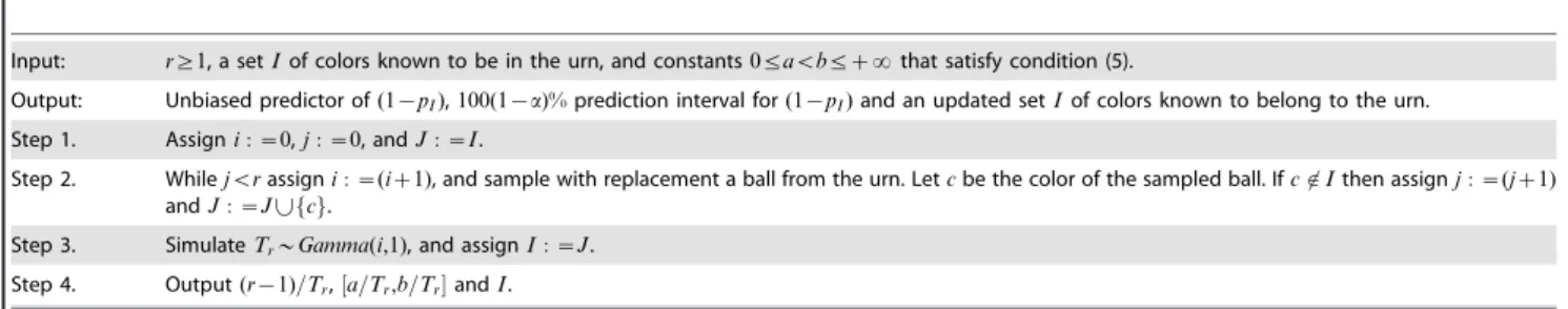
Table 1.Embedding algorithm.
Input: r§1, a setIof colors known to be in the urn, and constants0ƒavbƒz?that satisfy condition (5).
Output: Unbiased predictor of(1{pI),100(1{a)%prediction interval for(1{pI)and an updated setIof colors known to belong to the urn.
Step 1. Assigni:~0,j:~0, andJ:~I.
Step 2. Whilejvrassigni:~(iz1), and sample with replacement a ball from the urn. Letcbe the color of the sampled ball. Ifc6[Ithen assignj:~(jz1)
andJ:~J|fcg.
Step 3. SimulateTr*Gamma(i,1), and assignI:~J. Step 4. Output(r{1)=Tr,½a=Tr,b=TrandI.
(The term on the exponential on the left-hand side above is big-O of z3
a=2= ffiffiffiffiffiffiffiffiffiffi r{1 p
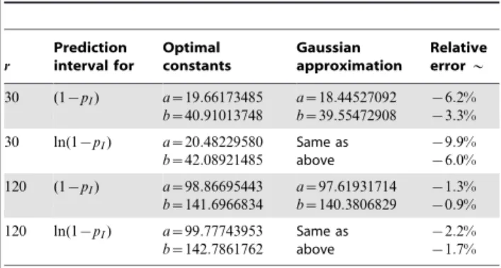
; in particular, the lower-bound is of the same asymptotic order than the upper-bound.) We note that the constants produced by the Normal approximation may be crude for relatively large values ofr, as seen in Table 2.
As high-throughput technologies allow deeper sampling of microbial communities, it will be increasingly important to have upper- and lower-bounds for (1{pI) of a comparable order of magnitude. Since the prediction intervals for this quantity in Theorem 2 are of the form½a=Tr,b=Tr, and the ratio between the upper- and lower-bound of this interval isb=a, one may wish to determine constantsaandbsuch that, not only (5) is satisfied, but also
b=a~f, ð9Þ
wherefw1is a user-defined parameter. Not all values off are attainable for a givenrand confidence level. In fact, the smallest attainable value is given by the constants associated with the optimal prediction interval for ln(1{pI). Equivalently, f is attainable if and only if
f§b=a, where ðb
a xr r!e
{xdx~(1{a)
and (a)re{a~(b)re{bwithavrvb:
Conversely, and as stated in the following result, any value offw1 is attainable at a given confidence level, provided that the parameterris selected sufficiently large.
Theorem 3Let0vav1andfw1be fixed constants. For each r sufficiently large, there are constants0vavbvz?such that (5) and (9) are satisfied.
For a given parameter f, there are at most two constants 0vc1vc2vz? such that ½c1=Tr,f:c1=Tr and ½c2=Tr,f:c2=Tr are prediction intervals for(1{pI)with exact confidence(1{a). We refer to these asconservative-lowerandconservative-upper prediction intervals, respectively. We refer to intervals of the form ½0,c0=Tr and ½c3=Tr,1 as upper- and lower-bound prediction intervals, respec-tively. See Table 3 for the determination of these constants for various values ofrwhena~5%.
Effect of non-randomized sample sizes
The Embedding algorithm provides conditionally unbiased predictors and intervals for(1{pI)and ln(1{pI), provided that an arbitrary number of additional observations is possible until observingr balls with colors outsideI. When dealing with fixed
sample sizes, there is a positive probability of not meeting this condition, in which case the Embedding Algorithm is inconclusive. In large samples however, such as those collected in microbial datasets, the algorithm may be applied sequentially until it yields an inconclusive prediction. In such case, the true confidence of the prediction intervals produced by the algorithm satisfy the following.
Theorem 4Suppose that condition (5) is satisfied. Conditioned onI, if rballs with colors outsideIare observed in the nextkdraws from the urn, then the true confidencec of the prediction interval for(1{pI) produced by the Embedding algorithm satisfies:
(i) ifa~0then(1{a)ƒcƒ(1{a)z ½Cwb;
(ii) ifaw0then(1{a){ ½Nwkƒcƒ(1{a)z ½Cwb,where Cis a Gamma random variable with parameters(r,1),andN is a Negative Binomial random variable with parameters(r,1{pI).
Table 2.Optimal versus asymptotic95%prediction intervals.
r
Prediction interval for
Optimal constants
Gaussian approximation
Relative error*
30 (1{pI) a~19:66173485
b~40:91013748
a~18:44527092
b~39:55472908
{6:2%
{3:3%
30 ln(1{pI) a~20:48229580 b~42:08921485
Same as above
{9:9%
{6:0%
120 (1{pI) a~98:86695443
b~141:6966834
a~97:61931714
b~140:3806829
{1:3% {0:9%
120 ln(1{pI) a~99:77743953
b~142:7861762
Same as above
{2:2%
{1:7%
doi:10.1371/journal.pone.0021105.t002
Table 3.Constants associated with 95% prediction intervals.
r c0 c1 c2 c3
1 2.995732274 0.051293294
2 4.743864518 0.355361510
3 6.295793622 0.817691447
4 7.753656528 0.806026244 1.360288674 1.366318397 5 9.153519027 0.924031159 1.969902541 1.970149568 6 10.51303491 1.053998892 2.61300725 2.613014744 7 11.84239565 1.185086999 3.28531552 3.285315692 8 13.14811380 1.315076338 3.98082278 3.980822786 9 14.43464972 1.443547021 4.69522754 4.695227540 10 15.70521642 1.570546801 5.42540570 5.425405697 11 16.96221924 1.696229569 6.16900729 6.169007289 12 18.20751425 1.820753729 6.92421252 6.924212514 13 19.44256933 1.944257623 7.68957829 7.689578292 14 20.66856908 2.066857113 8.46393752 8.463937522 15 21.88648591 2.188648652 9.24633050 9.246330491 16 23.09712976 2.309712994 10.03595673 10.03595673 17 24.30118368 2.430118373 10.83214036 10.83214036 18 25.49923008 2.549923010 11.63430451 11.63430451 19 26.69177031 2.669177032 12.44195219 12.44195219 20 27.87923964 2.787923964 13.25465160 13.25465160 21 29.06201884 2.906201884 14.07202475 14.07202475 22 30.24044329 3.024044329 14.89373854 14.89373854 23 31.41481021 3.141481021 15.71949763 15.71949763 24 32.58538445 3.258538445 16.54903872 16.54903871 25 33.75240327 3.375240328 17.38212584 17.38212584 Constants associated with95%upper-bound, lower, conservative-upper and lower-bound prediction intervals for(1{pI), when1ƒrƒ25andf~10. By definition, this means that
ðc0
0 xr{1 (r{1)!e
{xdx~0:95andð? c3
xr{1 (r{1)!e
{xdx~0:95.
Furthermore, the constantsc1ƒc2are solutions to the equation:
ð10c
c xr{1 (r{1)!e
{xdx~0:95, c§0,
solved numerically with Newton’s method using Maple 13.02. This equation may have at most two different solutions, and star () denotes that the equation has no solution.
Thus, if the Embedding algorithm produces an output in what remains of a finite sample size, the upper-bound prediction interval for(1{pI)has at least the user-defined confidence. This is perhaps the case of most interest in applications: it allows the user to estimate the least number of additional samples to observe a color not seen in any sample. For the other three interval types, the true confidence is approximately at least the targeted one if the probability that the algorithm produces an output in what remains of the sample is large.
Discussion
Comparisons with Robbins-Starr estimators
Note that, like Robbins’ and Starr’s estimators, our method requires extracting additional balls from the urn to make a prediction. However, unlike the methods of the Introduction, our method uses only the additionally collected data–instead of all the data ever collected from the urn–to make a prediction. In terms of sequential analysis, this is advantageous to recover from earlier erroneous predictions (we expand on this point in the next section, see Fig. 1).
In what remains of this section, I~fX1,. . .,Xng hence (1{pI)~Un, the conditional uncovered probability of a sample of size n. Furthermore, to rule out trivial cases, we assume that Unv1with positive probability i.e. the urn is composed by more than just balls of a single color.
Part (i) of Theorem 1 provides a conditionally unbiased predictor for Un. We can show, however, that Robbins’ and Starr’s estimators are not conditionally unbiased forUnin the non-parametric case when rvn=6z1. To see this argument, first notice thatjvn,r{vn,1jƒ3(r{1)=n due to the inequality (3). On the other hand, ifiis a color in the urn such thatpiw0then
(vn,1jI~fig)~1 {pi nz1:
As a result:
(1{pi){ (vn,rjI~fig)
~(1{pi){ (vn,1jI~fig)z (vn,1{vn,rjI~fig)
§1
2 1{ 6(r{1)
n {pi
:
Hence, if there exists a color iin the urn that makes the above quantity strictly positive (there are infinitely many such urns, including all urns composed by infinitely many colors, because rvn=6z1) thenvn,rcannot be conditionally unbiased forUn.
On the other hand, due to parts (i) and (ii) in Theorem 1, we obtain (see Materials and Methods):
r Un,r{1
Tr
~
ffiffiffiffiffiffiffiffiffiffiffiffiffiffiffiffiffiffiffiffiffiffiffiffiffiffiffiffi
(Un) ((r{1)=Tr)
s
, ð10Þ
r ln(Un),{ln(Tr){czX r{1 i~1 1
i !
~
ffiffiffiffiffiffiffiffiffiffiffiffiffiffiffiffiffiffiffiffiffi
(ln(Un)) (ln(Tr))
s
, ð11Þ
wherer denotes correlation and variance. Consequently, the point predictors in Theorem 1 are positively correlated with the quantities they were designed to predict. This contrasts with Robbins’ estimator, which may be strongly negatively correlated
withUn. For instance, ifpi~1=kforkdifferent colors in the urn, it is shown in [21] that the asymptotic correlation betweenUnand Robbins’ estimator vn,1 is asymptotically negative when n=k converges to a strictly positive but finite constantl. In this same regime but provided thatr% ffiffiffi
n p
, we can show that (see Materials and Methods):
limsup n??
r(Un,vn,r)ƒ
l:e{l{l:(1z3l):e{2l
2
ffiffiffiffiffiffiffiffiffiffiffiffiffiffiffiffiffiffiffiffiffiffiffiffiffiffiffiffiffiffiffiffiffiffiffiffiffiffiffiffiffiffiffiffiffiffiffiffiffiffiffiffiffiffiffiffiffiffiffiffiffiffiffiffiffiffiffiffiffiffiffiffiffiffiffiffiffiffiffiffiffi
l:e{2l{l:(2zl2):e{3lzl:(1zl3):e{4l
q : ð12Þ
Since the right-hand side above is negative for alll sufficiently small, Starr’s estimator vn,r may also have a strong negative correlation withUnwhenris much smaller than ffiffiffi
n p
.
A further calculation based on parts (i) and (ii) in Theorem 1 shows that
r{1
Tr
~ (Un)z (U
2 n) r{2 ,
(ln(Tr))~ (ln(Un))zX ?
i~r
1
i2:
In particular, for fixedn, the correlations in equations (10) and (11) approach to one asrtends to infinity.
Finally, for non-trivial urns with finite a-diversity, i.e. urns composed by balls with at least two but a finite number of different colors, one can show for fixedrthat the correlation in equation (10) approachespffiffiffiffiffiffiffiffiffiffiffiffiffiffiffiffiffiffiffiffiffiffiffiffiffiffiffi(r{2)=(r{1)
asntends to infinity. Further-more, if we again assume thatpi~1=kforkdifferent colors in the urn and n=k converges to a strictly positive but finite constant, then the correlation in equation (10) approaches zero from above. As we pointed out before, in this regime, Robbins’ estimator is asymptotically negatively correlated withUn.
Selection of parameters
There are two main criteria to select the parameter r of the Embedding algorithm in a concrete application.
One criteria applies for point predictors. In this case, conditioned onI, the standard deviation of the relative error of our prediction of (1{pI) is1= ffiffiffiffiffiffiffiffiffiffi
r{2 p
(Theorem 2, part (i)). To predict(1{pI),rshould be therefore selected as small as possible so as to meet the user’s tolerance on the average relative error of our predictions. The same criteria applies for point predictors of ln(1{pI), for which the standard deviation of the absolute error is of order1= ffiffi
r p
, uniformly for allpIv1(Theorem 2, part (ii)). A different criteria applies for prediction intervals. In this case, conditioned onI, the user should first specify the confidence level, and how much larger he wants the upper-prediction-bound to be in relation to the lower-prediction bound of (1{pI). Since the ratio between these last two quantities is given by the parameterf in (9),rshould be selected as small as possible to meet the user’s pre-specified factor f for the given confidence level of the prediction interval (Theorem 3). See Table 4 for the optimal choice ofrfor various values off whena~5%. Note that for the selected parameter r, the constants associated with the optimal prediction intervals are given in equations (6) and (7), see Materials and Methods.
Simulations on analytic and non-analytic urns
matching the observed distribution of microbes in a human-gut sample from [29]. We also analyzed a sample from a human-hand microbiota found in [30]. The gut and hand data are part of the largest microbial datasets collected thus far (see Fig. 4 for the relative abundance rank curve associated with each urn). The relative abundance rank curve, or for simplicity ‘‘rank curve’’, associated with an urn is a graphical representation of its composition: the height of the graph above a non-negative integer iis the fraction of balls in the urn with thei-th most dominant color.
The blue dots and red curves on the plots on the left side in Fig. 1 show very accurate point predictions in log-scale of the conditional uncovered probability (as a function of the number of observations), when we apply the Embedding algorithm to a sample of size50,000from the human-gut and exponential urn, respectively. In both instances, the parameterrof the Embedding algorithm was set to25. The accuracy of our method is confirmed by the red clouds on the plots on the right side of Fig. 1, which are centered around (1,1). The red clouds also indicate that our predictions recover more easily from offset predictions as compared to Robbins’ and Starr’s (correlation coefficient of red clouds,R~0:715451andR~0:244014on top- and bottom-right, respectively). This is to be expected because the Embedding algorithm relies only on the additionally collected data to make a new prediction, whereas Robbins’ and Starr’s estimators use all the data ever collected from the urn. On the other hand, the red and blue curves in Fig. 2 show that the conservativeupper and -lower prediction intervals of the conditional uncovered probability (also as a function of the number of observations) contain this quantity with high probability and, unlike Esty’s intervals, have a constant length in logarithmic scale. The intervals on the plots on the right side are tighter than those on the left because of the decrease of the parameter f from 2:5to1:5. In each case, the
Table 4.Optimal selection of parameterrin terms of parameterf.
f r c1 c2
80 2 0.0598276655 0.355361510
48 2 0.1013728884 0.355358676
40 2 0.1231379857 0.355320458
24 2 0.226833483 0.346045204
20 3 0.320984257 0.817610455
12 3 0.590243030 0.787721610
10 4 0.806026244 1.360288674
6 6 1.822307383 2.58658608
5 7 2.48303930 3.22806682
3 14 7.17185045 8.27008349
2.5 19 11.26109001 11.96814857
1.5 94 75.9077267 76.5492088
1.25 309 275.661191 275.949782
Constants associated with the controlled upper- to lower-bound ratio prediction intervals for(1{pI), whena~5%; in particular, for eachf andr, ½c1=Tr,f:c1=Trand½c2=Tr,f:c2=Trcontain(1{pI)with a95%probability. For
eachf, the smallest value ofrfor which the equation:
ðcf
c xr{1 (r{1)!e
{xdx~0:95, c§0;
admits a solution, is reported. Numerical values where determined using Maple 13.02.
doi:10.1371/journal.pone.0021105.t004
Figure 4. Rank curves associated with the human-gut, human-hand and exponential urn.In a rank curve, the relative abundance of a
species is plotted against its sorted rank amongst all species, allowing for a quick overview of the evenness of a community. On the left, rank curves associated with the human-gut (blue) and -hand data (green) show a relatively small number of species with an abundance greater than 1%, and a long tail of relatively rare species. The right rank curve of the exponential urn (red) simulates an extreme environment, where relatively excessive sampling is unlikely to exhaust the pool of rare species.
parameterrwas selected according to the guidelines in Table 4. We note that sequential predictions based on the Embedding Algorithm in figures 1 and 2 were produced until the algorithm yielded inconclusive predictions. For this reason, our predictions ended before exhausting each sample.
In the human-hand dataset, 163 species were observed in a sample of size5034. To simulate draws with replacement from this environment, we produced a random permutation of the data (see Materials and Methods section). Using the Embedding algorithm with parameters (r,f)~(50,2), and according to our point predictor, 133 of the species observed in the sample represent
*98:3%of that hand environment; in particular, the remaining
*1:7% is composed by at least 30 species. Furthermore, according to our upper-bound prediction interval, and with at least a95%confidence, the species not represented in the sample account for less than2:2%of that environment.
To test the above predictions, we simulated the rare biosphere as follows. We hypothesized that our point prediction of the conditional uncovered probability could be offset by up to one order of magnitude. We also hypothesized that the number of unseen species in the sample had an exponential relative abundance rank curve, composed either by 10, 100 or 1000 species. This leads to nine different urns in which to test our methods. These urns are devised such that they gradually change from the almost unchanged urn in the bottom left corner to the urn in the upper right, which is dominated by rare species (see Fig. 5 for the associated rank curves). As seen on the plots in Fig. 6, the Embedding algorithm yields very accurate predictions in each of these nine scenarios, for all the sample sizes considered.
As seen in Fig. 7, our predictions are also in excellent agreement with the human-gut dataset when we simulate the rare biosphere. As expected, the conditional uncovered probability almost always
lies between the predicted bounds. We also note that the predictions based on the Embedding algorithm are accurate even for a small number of observations. This suggests that our algorithm can be applied to deeply as well as shallowly sampled environments.
Materials and Methods
Heuristic behind the Embedding algorithm
The number of times a rare color occurs in a sample from an urn is approximately Poisson distributed. In the non-parametric setting, a direct use of this approximation is tricky because ‘‘rare’’ is relative to the sample size and the unknown urn composition. The embedding into a HPP is a way to accommodate for the Poisson approximation heuristic, without making additional assumptions on the urn’s composition. To fix ideas, imagine that no ball in the urn is colored black. Make up a second urn with a single ball colored black. We refer to this as the ‘‘black-urn’’. Now sample (with replacement) balls according to the following scheme: draw a ball from the original- versus black-urn with probabilityeand(1{e), respectively, whereew0is a fixed but small parameter. Under this sampling scheme, even the most abundant colors in the original-urn are rare. In particular, the smallereis, the closer is the distribution of the number of times a particular set of colors (excluding black) is observed to a Poisson distribution. This approach is not very practical, however, because the number of samples to observe a given number of balls from the original urn can be astronomically large wheneis very small. To overpass this issue imagine drawing a ball everye-seconds. Draws from the original urn will then be apart eTeseconds, whereTehas a Geometric distribution with mean1=e. As a result:lime?0z ½eTewt~exp({t), fortw0. Thus, asegets
smaller, the time-separations between consecutive samples from the
Figure 5. Rank curves associated with the rare biosphere simulation in the human-gut and -hand urn.Rank curves associated with Fig. 6
(green) and Fig. 7 (blue).
original urn resemble independent Exponential random variables with mean one. The black-urn can therefore be removed from the heuristic altogether by embedding samples from the original urn into a HPP with intensity one over the interval½0,z?).
Simulating draws with replacement
To simulate draws with replacement using data already collected from an environment, produce a random permutation of the data. This can be accomplished with low-memory complexity using the discrete inverse transform method to simulate draws–without replacement–from a finite population [31].
Constants associated with optimal prediction intervals
To numerically approximate a pair of constants0vavbv?
such that Ðb ax
ke{x=k!dx~c and ake{a~bke{b, where the integer k§1 and the number 0vcv1 are given constants, introduce the auxiliary variable t~b=a, and note that the later condition is fulfilled only whena~k:ln(t)=(t{1)andb~t:a. Due to Newton’s method, the sequence(tn)n§0defined recursively as follows converges to the unique t that satisfies the integrability condition, provided thatt0is chosen sufficiently close tot:
an~k :ln(tn)
tn{1 ;
bn~tn:an;
tnz1~tn 1{ (k{1)! ak
n:e{an : ðbn
an xk k!e
{xdx{c
:
Proof of Inequality (3)
First notice that
jvn,1{vn,rjƒ
N(1,nz1)
nz1 {
N(1,nzr)
nzr
zX
r
k~2 r{1
k{1
!
nzr
k
!:N(k,nzr):
ð13Þ
To bound the first term on the right-hand side above, notice that jN(1,nz1){N(1,nzr)jƒ(r{1). As a result, since N(1,nzr)ƒ(nzr), we obtain that:
N(1,nz1)
nz1 {
N(1,nzr)
nzr
~N(1,nz1){N(1,nzr)
nz1 zN(1,nzr) 1
nz1{ 1
nzr
,
ƒr{1 n{1z
N(1,nzr)
nzr :r{1
nz1ƒ
2(r{1)
nz1 :
ð14Þ
On the other hand, to bound the second term on the right-hand side of equation (13), define the quantityN~Prk~2k:N(k,nzr) and notice that NƒPnkz~r1k:N(k,nzr)ƒ(nzr). Using that a
Figure 6. Predictions in the human-hand urn when simulating the rare biosphere.Prediction of the conditional uncovered probability
(black) in nine urns associated with a human-hand urn. Point predictions produced by the Embedding algorithm (blue), point predictions produced
by the algorithm each time a new species was discovered (red),95%upper-bound interval (orange), and95%conservative-upper interval (green). The
algorithm used the parameters (r,f)~(50,2). The different urns were devised as follows. For each i~0:17,0:017,0:0017 (indexing rows) and
j~10,100,1000(indexing columns), a mixture of two urns was considered: an urn with the same distribution as the microbes found in a sample from
a human-hand and weighted by the factor(1{i), and an urn consisting ofjcolors (disjoint from the hand urn), with an exponentially decaying rank
curve and weighted by the factori. See Fig. 5 for the rank curve associated with each urn.
weighted average is at most the largest of the terms averaged, we obtain that:
Xr
k~2 r{1
k{1
!
nzr
k
!:N(k,nzr)
~ N
nzr: Xr
k~2
(nzr) r
{1
k{1
!
k n
zr
k
! :
k:N(k,nzr)
N ,
ƒ max
2ƒkƒr
(nzr) r
{1
k{1
!
k n
zr
k
! ,
~ max
2ƒkƒr
P
k{1 i~1
r{kzi r{kziznƒ
r{1
r{1zn,
ð15Þ
where, for the last inequality, we have used that for eachk, the associated product is less or equal to the factor associated with the
index i~(k{1). Equation (3) is now a direct consequence of equations (13), (14) and (15).
Proof of Theorem 1
In what follows,f{1denotes the inverse function off. DefineM to be the set of decreasing partitions ofni.e. vectors of the form(i1,. . .,ik), with k§1and i1§ §ik§1integers, such thati1z. . .zik~n. To each possible sample(x1,. . .,xn), letg(x1,. . .,xn)be the decreasing partition ofnassociated with the observed ranks in the sample.
Define pI~Pi[Ipi, for each set I of colors. Part (i) in the theorem is equivalent to the existence of a function h:M?½{?,?such that
½h(g(X1,. . .,Xn))j(X1,. . .,Xn)~f(pfX1,...,Xng), ð16Þ
with probability one. This is because, in the non-parametric setting, the different colors in the urn carry no intrinsic meaning apart from being different. If there is a certain functionhwhich satisfies condition (16) thenf{1(h((n)))~pi, for each colorisuch thatpiw0. In particular, the setfj§1such that pjw0gmust be finite. Furthermore, if this set has cardinalityl thenpj~1=l, for each colorjin the set; in particular,f{1(h((n)))~1=l. Condition (ii) is therefore necessary for condition (i). Conversely, if condition (ii) is satisfied and the urn is composed bylcolors occurring in
Figure 7. Predictions in the human-gut urn when simulating the rare biosphere.In a sample of size12,903from a human-gut,123species
were discovered. Based on our methods, we estimate that97of these species represent*99:4%of that gut environment; hence, the remaining
*0:6%is composed by at least26species. To test our predictions of the conditional uncovered probability (black), we simulated the rare biosphere
by adding additional species and hypothesized that our point prediction could be offset by up to one order of magnitude: point predictions
produced by the Embedding Algorithm (blue), point predictions produced by the algorithm each time a new species was discovered (red),95%
upper-bound (orange), and95%conservative-upper interval (green). The predictions used the parameters(r,f)~(50,2). The different urns were
devised as follows. For eachi~0:06,0:006,0:0006(indexing rows) andj~10,100,1000(indexing columns), a mixture of two urns was considered: an urn with the same distribution as the microbes found in the gut dataset, and weighted by the factor(1{i), and an urn consisting ofjcolors (disjoint
from the gut urn), with an exponentially decaying rank curve and weighted by the factori. See Fig. 5 for the rank curve associated with each urn.
equal proportions then the functionh:M?½{?,?defined as h(i1,. . .,ik)~f(k=l)satisfies condition (16).
Proof of Theorem 2
Conditioned on the setI, and the random indexiused in Step 3 of the Embedding algorithm,Trhas a Gamma distribution with shape parameteriand scale parameter1. However, becauseihas a Negative Binomial distribution, conditioned onI alone,Trhas Gamma distribution with shape parameterrand scale parameter 1=(1{pI). In particular, (1{pI):Tr has probability density functionxr{1e{x=(r{1)!, forx§0. From this, parts (i) and (iii) in the theorem are immediate. To show part (ii), notice first that Lr~(cr{ln(Tr))is conditionally unbiased forln(1{pI), where
cr~ ð?
0 ln(x):x
r{1e{x
(r{1)! dx~
1
r{1zcr{1:
The second identity above is due to an integration by parts argument and only holds for r§2. However, since c1~{c, we obtain thatcr~{czPri~{111=i, forr§1. This shows that Lr is conditionally unbiased forln(1{pI). To complete the proof of the theorem, notice that Lr and ln((1{pI):Tr) have the same variance. In particular, (Lr)~dr{c2r, where
dr~ ð?
0
(ln(x))2:x
r{1e{x
(r{1)! dx~
2cr{1 r{1zdr{1:
The last identity above holds only for r§2. Using that d1~c2zp2=6, we conclude that dr~c2zp2=6z2Pr
{1 i~1ci=i, for r§1. As a result: (Lr)~p2=6{Pr{1
i~11=i2; in particular, sinceP?
i~11=i2~p2=6, (Lr)~ P?
i~r1=i2. The theorem is now a consequence of the following inequalities:
1
r~ ð?
r
1
x2dxƒ (Lr)ƒ ð?
r{1 1
x2dx~ 1
r{1:
Proof of Equation (8)
Letz~za=2and assume that0vzv ffiffiffiffiffiffiffiffiffiffi r{1 p
. Observe that:
c~ ffiffiffiffiffiffi
2p p
(r{1)r{1=2e1{r
(r{1)!
:ðz
{z e{x ffiffiffiffiffiffiffir
{1
p
ffiffiffiffiffiffi
2p
p 1z x ffiffiffiffiffiffiffiffiffiffi r{1
p
r{1
dx:
The factor multiplying the previous integral is an increasing function ofr; in particular, due to Stirling’s formula, it is bounded by 1 from above. Furthermore, from section 6.1.42 in [32], it follows that
e
{1 12(r{1)ƒ
ffiffiffiffiffiffi
2p p
(r{1)r{1=2e1{r
(r{1)! ƒ1:
On the other hand, if one rewrites the integrand of the previous integral in an exponential-logarithmic form and uses that y{y2=2zcz,r=(r{1)ƒln(1zy)ƒy{y2=2zy3=3, for all y§ {z= ffiffiffiffiffiffiffiffiffiffi
r{1 p
, where
cz,r~z: ffiffiffiffiffiffiffiffiffiffi r{1 p
zz
2
2z(r{1):ln 1{
z ffiffiffiffiffiffiffiffiffiffi r{1 p
,
one sees that
ecz,r{x2=2ƒe{xpffiffiffiffiffiffiffir{1
1z x ffiffiffiffiffiffiffiffiffiffi r{1 p
r{1
ƒe z3 3 ffiffiffiffiffiffiffir
{1
p {x2=2
:
All together, these inequalities imply that
ecz,r{12(r1{1) ðz
{z e{x2=2
ffiffiffiffiffiffi
2p
p dxƒcƒe z3
3 ffiffiffiffiffiffiffiffiffiffi
r{1
p ðz
{z e{x2=2
ffiffiffiffiffiffi
2p p dx,
from which the result follows.
Proof of Theorem 3
Due to the Central Limit Theorem, if c(r)~r{pffiffir:z a=4 and b(r)~rzpffiffir:z
a=4then
lim
r?? ðb(r)
c(r)
xr{1e{x
(r{1)! dx~1{
a 2:
As a result, for all r sufficiently large, 0ƒb(r)ƒf:c(r), and the integral on the left-hand side above is greater than or equal to (1{a). Fix any suchr. Since the value of the associated integral may be decreased continuously by increasing the parameterc(r), there isa(r)such thatc(r)ƒa(r)ƒb(r)and
ðb(r)
a(r) xr{1e{x
(r{1)! dx~(1{a):
Define g(t)~Ðf
:t t xr
{1e{x=(r{1)!dx, for t§0. Since g(0)~0 and, becauseb(r)ƒa(r):f,g(a(r))§(1{a), the continuity ofg(:) implies that there is0ƒtƒa(r)such thatg(t)~(1{a). Selecting a~tandb~f:tshows the theorem.
Proof of Theorem 4
The proof is based on a coupling argument. First observe that one can define on the same probability space random variables M,N,E1,E2,. . .such that (1)M and N have Negative Binomial distributions with parameters(r,1{pI), but withM conditioned to be less than or equal tok; (2)MƒN butM~NwhenNƒk; and (3)E1,E2,. . .are independent Exponentials with mean1and independent of(M,N).
LetAbe the event ‘‘rballs with colors outsideIare observed in the nextkdraws from the urn’’. Conditioned onI, we have that c~ ½aƒ(1{pI):TrƒbjA and (1{a)~ ½aƒ(1{pI):Trƒb. As a result:
c~ a
1{pIƒ XM
i~1
Eiƒ b
1{pI
" #
;
(1{a)~ a
1{pIƒ XN
i~1
Eiƒ b
1{pI
" #
:
SincePMi~1Eiƒ PN
i~1Ei, and becauseM~N when Nƒk, we obtain that
{ ½Nwkƒc{(1{a)ƒ b
1{pIv XN
i~1 Ei
" #
From this, the upper-bound in part (i) and both inequalities in part (ii) follow after noticing thatPNi~1Ei has a Gamma distribution with shape parameterrand scale parameter1=(1{pI). To show the lower-bound in (i), we again notice thatPMi~1Eiƒ
PN i~1Ei. In particular, ifa~0then
c{(1{a)~ X M
i~1
Eiƒ b
1{pI
" #
{ X
N
i~1
Eiƒ b
1{pI
" #
§0:
Proof of Equations (10) and (11)
Consider random variablesXandYand a random vectorZ, de-fined on a same probability space. Assume thatXis square-integrable and conditionally unbiassed for Y given Z i.e. (XjZ)~Y. Furthermore, assume that (Y)w0hence (X)w0. BecauseYis also square-integrable and (X)~ (Y), we obtain that
cov(X,Y)~ ((X{ (Y)):(Y{ (Y))),
~ ( (X{ (Y)jZ):(Y{ (Y))),
~ ((Y{ (Y))2)~ (Y):
Hencer(X,Y)~pffiffiffiffiffiffiffiffiffiffiffiffiffiffiffiffiffiffiffiffiffiffiffiffiffiffi(Y)= (X).
Equation (10) follows by considering X~(r{1)=Tr, Y~Un and Z~(X1,. . .,Xn). Similarly, equation (11) follows by
consid-eringX~{ln(Tr){czPri{~111
i andY~ln(Un).
Proof of Inequality (12)
First note that
r(Un,vn,r)~
cov(Un,vn,r{vn,1)zcov(Un,vn,1) ffiffiffiffiffiffiffiffiffiffiffiffiffiffiffiffiffiffiffiffiffiffiffiffiffiffiffiffiffi
(Un): (vn,r)
p ,
ƒ (fvn,r{vn,1g
2
)=2z (Un)=2zcov(Un,vn,1) ffiffiffiffiffiffiffiffiffiffiffiffiffiffiffiffiffiffiffiffiffiffiffiffiffiffiffiffiffi
(Un): (vn,1)
p :
ffiffiffiffiffiffiffiffiffiffiffiffiffiffiffi
(vn,1) (vn,r) s
:
ð17Þ
Now observe that (fvn,r{vn,1g2)~O(r2=n2) because of in-equality (13), which implies that n: (fvn,r{vn,1g2)~o(1) because r%pffiffiffin. On the other hand, because Robbins’ and Starr’s estimators are both unbiased for un, we have
j ffiffiffiffiffiffiffiffiffiffiffiffiffiffi
(vn,r) p
{ ffiffiffiffiffiffiffiffiffiffiffiffiffiffiffi(vn,1) p
jƒ
ffiffiffiffiffiffiffiffiffiffiffiffiffiffiffiffiffiffiffiffiffiffiffiffiffiffiffiffiffiffiffiffi
(fvn,r{vn,1g2) q
. Furthermore,
ac-cording to the proof of Theorem 2 in [21], (vn,1)~H(n{1), therefore
ffiffiffiffiffiffiffiffiffiffiffiffiffiffiffi
(vn,r)
(vn,1) s {1
~O rffiffiffi n p
:
As a result,limn??
ffiffiffiffiffiffiffiffiffiffiffiffiffiffiffiffiffiffiffiffiffiffiffiffiffiffiffiffiffiffiffi
(vn,1)= (vn,r) p
~1. Inequality (12) is now a direct consequence of inequality (17), and the next identities [21]:
lim
n??n
: (Un)~l:e{l{l:(1zl):e{2l;
lim
n??n
:cov(Un,vn,1)~{l2:e{2l;
lim
n??n
: (vn,1)~e{l{(1{lzl2):e{2l:
Acknowledgments
We would like to thank three anonymous referees for their careful reading of our manuscript and their numerous suggestions, which were incorporated in this final version. The authors are also thankful to R. Knight for contributing to an early version of the code, implementing some of the analyses, and commenting on the manuscript.
Author Contributions
Directed the research project: ML. Developed the new statistical method and accompanying mathematics: ML RG. Implemented the methods: JR. Designed the plots: JR ML. Generated the plots: JR. Wrote the manuscript: ML RG.
References
1. Sogin ML, Morrison HG, Huber JA, Welch DM, Huse SM, et al. (2006) Microbial diversity in the deep sea and the underexplored \rare biosphere’’. Proc Natl Acad Sci USA 103: 12115–12120.
2. Hughes JB, Hellmann JJ, Ricketts TH, Bohannan BJ (2001) Counting the uncountable: statistical approaches to estimating microbial diversity. Appl Environ Microbiol 67: 4399–4406.
3. Schloss PD, Handelsman J (2004) Status of the microbial census. Microbiol Mol Biol Rev 68: 686–691.
4. Curtis TP, Head IM, Lunn M, Woodcock S, Schloss PD, et al. (2006) What is the extent of prokaryotic diversity? Phil Trans R Soc Lond 361: 2023–2037. 5. Roesch LF, Fulthorpe RR, Riva A, Casella G, Hadwin AK, et al. (2007)
Pyrosequencing enumerates and contrasts soil microbial diversity. Isme J 1: 283–290.
6. Hong SH, Bunge J, Jeon SO, Epstein SS (2006) Predicting microbial species richness. Proc Natl Acad Sci USA 103: 117–122.
7. Quince C, Curtis TP, Sloan WT (2008) The rational exploration of microbial diversity. Isme J 2: 997–1006.
8. Turnbaugh PJ, Hamady M, Yatsunenko T, Cantarel BL, Duncan A, et al. (2007) A core gut microbiome in obese and lean twins. Nature 457: 480–484. 9. Fierer N, Lauber CL, Zhou N, McDonald D, Costello EK, et al. (2010) Forensic
identification using skin bacterial communities and/or references within. Proc Natl Acad Sci USA 107: 6477–6481.
10. Magurran AE (2004) Measuring Biological Diversity Oxford - Blackwell. 11. Burnham KP, Overton WS (1978) Estimation of the size of a closed
popu-lation when capture probabilities vary among animals. Biometrika 65: 625– 633.
12. Chao A (1984) Nonparametric estimation of the number of classes in a population. Scand J Stat 11: 265–270.
13. Chao A (1897) Estimating the population size for capture-recapture data with unequal catchability. Biometrics 43: 783–791.
14. Mao CX, Lindsay BG (2007) Estimating the number of classes. Ann Stat 35: 917–930.
15. Bunge J, Fitzpatrick M (1993) Estimating the number of species: A review. J Am Stat Assoc 88: 364–373.
16. Hinsley F, Stripp A (1993) Codebreakers: The Inside Story of Bletchley Park Oxford Univ. Press.
17. Finch SJ, Mendell NR, Thode Jr. HC (1989) Probabilistic measures of adequacy of a numerical search for a global maximum. J Am Stat Assoc 84: 1020–1023. 18. Mao CX (2004) Predicting the conditional probability of discovering a new class.
J Am Stat Assoc 99: 1108–1118.
19. Good IJ (1953) The population frequencies of species and the estimation of population parameters. Biometrika 40: 237–264.
21. Starr N (1979) Linear estimation of the probability of discovering a new species. Ann Stat 7: 644–652.
22. Clayton MK, Frees EW (1987) Nonparametric estimation of the probability of discovering a new species. J Am Stat Assoc 82: 305–311.
23. Esty WW (1983) A Normal limit law for a nonparametric estimator of the coverage of a random sample. Ann Statist 11: 905–912.
24. Aldous D (1988) Probability Approximations via the Poisson Clumping Heuristic Springer-Verlag.
25. Mahmoud HM (2000) Sorting: A Distribution Theory Wiley-Interscience. 26. Hwang HK, Janson S (2008) Local limit theorems for finite and infinite urn
models. Ann Probab 36: 992–1022.
27. Mao CX, Lindsay BG (2002) A poisson model for the coverage problem with a genomic application. Biometrika 89: 669–681.
28. Durrett R (1999) Essentials of stochastic processes Springer Texts in Statistics. 29. Turnbaugh PJ, Ridaura VK, Faith JJ, Rey FE, Knight R, et al. (2009) The e_ect
of diet on the human gut microbiome: A metagenomic analysis in humanized gnotobiotic mice. Sci Transl Med 1: 6ra14.
30. Fierer N, Hamady M, Lauber CL, Knight R (2008) The influence of sex, handedness, and washing on the diversity of hand surface bacteria. Proc Natl Acad Sci USA 105: 17994–17999.
31. Ross SM (2002) Simulation Academic Press, third edition.