Choosing the best method of depreciating assets and after-tax economic analysis under uncertainty using fuzzy approach

(1)

Contents lists available at GrowingScience

Decision Science Letters

homepage: www.GrowingScience.com/dsl

Choosing the best method of depreciating assets and after-tax economic analysis under uncertainty using fuzzy approach

Saeed Khalilia*, Yahia Zare Mehrjerdib and Hassan Khademi Zarec

a

Saeed Khalili, MSc. Student, Industrial Engineering Department, Yazd University, Yazd, Iran b

Yahia Zare Mehrjerdi, Associate Professor, Industrial Engineering Department, Yazd University, Yazd, Iran c

Hassan Khademi Zare, Associate Professor, Industrial Engineering Department, Yazd University, Yazd, Iran C H R O N I C L E A B S T R A C T

Article history:

Received January 14, 2014 Accepted July 7, 2014 Available online August 7 2014

In the past, different methods for asset depreciation have been defined but most of these procedures deal with certain parameters and inputs. The availability of certain parameters in many real world situations is difficult and sometimes impossible. The primary objective of this paper is to obtain methods for calculating depreciation where some of the defined parameters are under uncertainty. Hence, by using the fuzzy science basics, extension principle and α-cut technique, we rewrite some classic methods for calculating depreciation in fuzzy form. Then, for comparing the methods of fuzzy depreciation under uncertain conditions by using the formula of calculating the Fuzzy Present worth (FPW), the Present worth of Tax saving (PWTS) of any aforementioned methods has been obtained. Finally, since the amount of tax savings achieved for each of the methods is a fuzzy number, one of the fuzzy prioritization methods is used in order to select the best depreciation technique.

Fuzzy Depreciation Extension Principle α-cut Technique Fuzzy Present Worth of Tax Saving

Fuzzy Prioritization Techniques

1. Introduction

(2)

458

3 discusses classical and fuzzy depreciation methods used in this article. Section 4 offers the formula for calculating fuzzy Present worth of tax savings_{(PW )}. Ranking fuzzy numbers is the topic of section 5. In section 6, a numerical example is presented for clarification purposes. Author's conclusion is given in section 7.

2. Literature Review

In relation to the choice of depreciation methods, a number of researches can be noted (Davidson & Drake, 1961, 1964; Roemmich et al., 1978; Wakeman, 1980). In these researches, future cash flows have enough certainty to cover the amount of depreciation. Wakeman (1980) analytically showed that the Accelerated Depreciation Method (ADM) for any value of the discount rate in the range [0, 1] excels Straight Line Depreciation Method (SLDM)ٰ. This is because ADM has lower Present Worth (PW) of tax payment compared to (SLDM). Berg and Moore (1989) state that (SLDM) is a comprehensive and preferred method of depreciation. Wielhouwer et al. (2002) investigated the optimal tax depreciation under progressive tax system. Jackson et al. (2009) examined the economic consequences of choosing certain depreciation methods for companies. Berg et al. (2001) presented a method for optimization of tax depreciation under uncertainty conditions of future cash flows. They compared Sum of year digits (SOYD), double declining balance (DDB), (SLDM) and (ADM) depreciation methods and examined the effects of factors such as discount rate, future cash flow rate and tax system structure on the choice of optimal depreciation method. Nevertheless, up until now there has been no great attention to the application of fuzzy logic in the field of economy. In addition, any attempt to use fuzzy approach for choosing the best depreciation method in terms of uncertainty conditions has not been accomplished. From the few researches on using fuzzy logic in economic calculations, following researches can be noted. Moradi et al. (2012) offered a solution procedure for

comparing projects using optimal α-cut method when there are several Internal Rates of Returns

(IRR). For solving political and economic instability problem, Ameli et al. (2013) proposed a model for calculating the Economic Order Quantity (EOQ) considering discounted rate and inflation rate as fuzzy numbers. Kahraman et al. (2002) in their article originally stated the importance of risk and uncertainty in the economy and argued that in these conditions, even knowledge of experts are prone to errors. They state that rates and amount of cash flows are usually obtained from strong conjectures from the data. Therefore, fuzzy numbers can help this topic and continues to provide a model for the application of fuzzy logic in engineering economy. In another article, while comparing stochastic and fuzzy methods, Kahraman (2001) concluded that the application of probability theory in economic evaluation requires a relatively large number of historical data about the income, costs and interest rated, while the fuzzy logic can formulate uncertainty without needing that much data. Huang (2008) presented a model for calculating net present value by using random fuzzy numbers and Hybrid Intelligent Algorithm. Chiu and Park (1994) presented a method for calculating the Fuzzy Present worth (FPW) and Fuzzy Future worth (FFW). Shahriari (2011), using the extension principle (Zadeh, 1978) presented a method of calculating Fuzzy Net Present Value (FNPV), while interest rate (i) and the annual cash flow are considered uncertain. He also used fuzzy Delphi method for obtaining each year’s interest rate. Due to the presence of uncertainty in input data, Kahraman and Kaya (2008) considered a triangular fuzzy number for depreciation and the cash flow. Then, by changing the fuzzification ratio, they have calculated the rate of return for after-tax cash flow as a fuzzy number using SOYD and SL depreciation methods. Considering the lack of a proper solution to choose the optimal depreciation method under conditions of uncertainty, we have presented a model in this paper that has combined classical methods of calculating depreciation and fuzzy logic to overcome this problem.

3. Research methods and steps

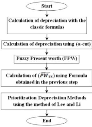
This research method is comprised of following steps:

(3)

Step 2: Due to uncertainty in some parameters, we will rewrite formulas of calculating depreciation in

Fuzzy form using Interval Arithmetic and alpha cut (α-cut) method.

Step 3: We presented a formula for Fuzzy Present worth (FPW) using Zadeh's extension principle.

Step 4: We have calculated the amount of present worth of tax savings for all depreciation methods to choose the best method of depreciation.

Step 5: the fuzzy prioritization technique of Lee and Li (1988) are described for comparison of depreciation methods. These steps are shown in Fig. 1.

Fig. 1. Flowchart of Research methods and steps

3.1. Classical and fuzzy methods for calculating depreciation

Various methods have been proposed to depreciate assets. In the following section, some of the most important and useful methods of these will be discussed.

3.1.1. Straight-line depreciation method

The straight line method is probably the simplest and most common method for calculating depreciation. In this method, the annual depreciation is constant and is obtained from Eq. (1).

= , =1,2,…., (1)

where is the amount of depreciation in year j, Pis the initial cost of asset, SV is the salvage value of asset and n is the number of years of assets’ useful life. The parameters n and SV are uncertain therefore domain experts express their predictions about these parameters. Since these are in the form of linguistic variables like (almost 10 years, or approximately 20%), for any of these parameters a fuzzy triangular number is defined. Finally, using fuzzy Delphi method (Chang et al., 2000), to reach a consensus, we consider triangular fuzzy number _sv = (sv1 , sv2 , sv3) for the amount of SV and triangular fuzzy numbern = (n1 , n2 , n3) for the amount of n. Then, using the concepts of interval

mathematical and α-cut method and fuzzy mathematical operations for triangular fuzzy numbers

(Buckley, 2004), we will rewrite the classical depreciation formulas as fuzzy.

3.1.2. Fuzzy Straight-line depreciation method with fuzzy parameters and :

SV= (SV,SV ,SV ) (2)

= (N ,N ,N ) (3)

(4)

460

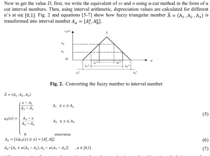
Now to get the value D, first, we write the equivalent of sv and nusing α-cut method in the form of α cut interval numbers. Then, using interval arithmetic, depreciation values are calculated for different

α’s at α_∈[0,1]. Fig. 2 and equations [5-7] show how fuzzy triangular number _{A = (A} _{, A} _{, A )} is

transformed into interval number = [ , A ].

Fig. 2. Converting the fuzzy number to interval number

= ( , , )

( ) =

⎩ ⎪ ⎪ ⎨ ⎪ ⎪

⎧ −₋ ≤ ≤

−

− ≤ ≤

0 ℎ

(5)

= { | ( )_≥ } = [ , ] ₍₆₎

=[ + ( − ), − ( ₋ )] , ∈[0,1] ₍₇₎

After converting fuzzy numbers to interval numbers, using intervals arithmetic, calculations are done easily. If _{= [} _, ] , = [ , ], then:

A + B=[ + , + ] (8)

A−B=[ − , − ] (9)

A. B=[ . , . ] (10)

A ÷ B= , (11)

K. A=[ , ]. [ , ] = [ , ] (12)

According to the above calculations, depreciation values are calculated by Eq. (15):

SV= (SV,SV ,SV ) ⟹SV =[SV ,SV ] = [SV +Α(SV −SV),SV −Α(SV −SV )] (13)

= ( , , )⟹ =[ , ] = [ + ( − ), − ( − )] (14)

⟹ = [ , ] = , ∈[0,1] (15)

3.2. Sum of Year Digits Depreciation Method

(5)

=( ( ))( − ) =1,2,…., (16)

= ( , , )⟹ =[ , ] = [ + ( − ), − ( − )] ₍₁₇₎

= ( , , )⟹N =[N ,N ] = [ + ( − ), − ( − )] ₍₁₈₎

⟹ = , = 2 − + 1

( + 1) ( − ), 2

− + 1

( + 1) ( − ) ∈[0,1]

(19)

3.3. Double Declining Balance depreciation method (DDB)

In addition, in this method like the method of Sum of the Year Digits, the amount of depreciation in the first year is the most and decreases with a fixed rate every year. The depreciation value of every year is obtained from Eq. (20).

=( ) = 1,2, … . , (20)

BV is the book value of (t-1)th year and is obtained from Eq. (21).

= (1−2) _{= 1,2, … . ,} (21)

Therefore, the depreciation value is calculated according to Eq. (22).

=( )(1− ) = 1,2, … . , (22)

Due to the fuzziness of n, depreciation value is calculated in Eq. (24).

= ( , , )⟹ =[ , ] = [ + ( − ), − ( − )] ₍₂₃₎

⟹ = , = 1− , 1− ∈[0,1] (24)

3.4. Sinking fund depreciation method (SFDM)

Unlike two methods described previously, this method is such that the lowest amount of depreciation is in the first year and gradually increases, so that in the final year it will be the maximum amount of depreciation. In this method the depreciation value in jth year is obtained from Eq. (25) that in addition to n and sv, i j is fuzzy. ( ) is the interest rate at jth year. In this method, fuzzy depreciation value is obtained from Eq. (29).

=( )( ) ( ) = 1,2, … . , (25)

= ( , , )_⟹ =[ , ] = [ + ( − ), ₋ ( ₋ )] ₍₂₆₎

= ( , , )⟹ =[ , ] = [ + ( − ), − ( − )] ₍₂₇₎

= , , ⟹ = , = + − , − − (28)

⟹ = , = ( ( ) ( ) ), ( ( ) ( )) ∈[0,1] (29)

4. Fuzzy present worth method (FPW)

We must choose the optimum method for depreciation so that it has the maximum rate of tax savings. Tax saving in jth year is obtained from Eq. (30).

= . ( ) ₍₃₀₎

In Eq. (30), is the symbol for tax savings in the jth year, represents the depreciation value and

(6)

462

tax savings of a particular year should not be the criteria, but tax savings achieved over the entire range of asset’s life should be considered. Therefore, the index, Present Worth of tax savings(PW ), that shows tax savings throughout the lifetime of the asset is included and can be used to compare and choose the best method of depreciation (Blank et al., 2005). If we show Interest rates in the jth year as

ij, the classic formula for the present Worth of tax savings is stated by Eq. (31).

= . ( ) , , 1 = . ( ) ( 1

1 + )

(31)

Given the amount of depreciation and interest rates in the jth year (D and ) and duration of life (n) are fuzzy parameters and are obtained using the principle of Zadeh, the fuzzy formulation of the present worth of tax savings is shown in Eq. (33):

= ( , , ), _̃ = , , , = , , (32)

= , , = . ( ) 1

1 + , . ( ) ( 1

1 + ) , . ( ) ( 1 1 + )

(33)

5. Ranking fuzzy numbers

Now, given the present worth tax savings obtained from each of the different methods of depreciating assets in the form of triangular fuzzy numbers, for selecting best depreciation method, we will need to use a prioritization method for fuzzy numbers. Ranking of fuzzy numbers is based upon one or several different feature of fuzzy numbers. This feature may be the Center of Gravity, the area under the membership function, or the points of intersection between the sets. A ranking method considers the distinctive features of fuzzy numbers and ranks them based upon these. Therefore, it is reasonable that for the same group of fuzzy numbers, different methods of ranking fuzzy numbers yield different rankings. Variety of methods has been proposed for prioritizing fuzzy numbers (Asady, 2010; Asady & Zendehnam, 2007; Cheng, 1998; Chu & Tsao, 2002; Nejad & Mashinchi, 2011; Wang & Lee, 2008). We have employed the Lee and Li (1988) method of prioritizing fuzzy numbers in this article. In this method, fuzzy numbers are compared using two criterions: (1) fuzzy number mean and (2) fuzzy number dispersion. They have calculated the dispersion by the standard deviation (sd). It is assumed that a fuzzy number with greater mean and less standard deviation has higher priority for the decision maker. For proportional distribution, mean and standard deviation value of fuzzy number is obtained from Eq. (34) and Eq. (35).

= ∫

( )

∫ ( )

(34)

= ∫( ) ( ( ))

∫₍ ₎( ( )) −( )

(35)

Eqs. (34-35) would be converted to Eqs. (36-37), if is a triangular fuzzy number as _{= ( ,} _{. )}.

= 1

4( + 2 + )

(36)

= 1

80(3 + 4 + 3 −2 −4 −4 )

(37)

(7)

Table 1

Ranking fuzzy numbers

Comparison of mean values Comparison of sd values Prioritization result

( ) > ( ) >

( ) = ( ) ( ) < ( ) >

6. Numerical example

Assume that a factory has purchased a new machine with about 3 years useful life and an initial value of 10000 units. In accordance with experts opinion the salvage value (sv) of this machine is approximately 2000 units. It is assumed that the tax rate (TR) are 10%, 20%, 30%, and 40% during these four years periods. Our experts’ opinion indicates that interest rates are approximately 10%, 15%, 20% and 25%, for years 1 through 4. There is no regulation on selecting an appropriate form of depreciation for this company. Now, the question is what is the best method of depreciation that management must choose to depreciate this asset? Due to the fact that some of the parameters used in this study are in the form of linguistic variables (around, about, etc.) as predicted by our in house experts, therefore we will use fuzzy theory. We have allocated appropriate triangular fuzzy numbers to each of these parameters according to the Table 2.

Table 2

Transforming linguistic variables to fuzzy numbers

Triangular fuzzy variables Experts linguistic variables Problem parameters

Triangular fuzzy variables Experts linguistic variables Problem parameters (5%,10%,15%) Approximately 10% ( ) (2,3,4) About 3 years

(10%,15%,20%) Approximately 15% ( ) (10000,10000,10000) 10000 P (15%,20%,25%) Approximately 20% ( ) (1000,2000,3000) Approximately 2000 units

(20%,25%,30%) Approximately 25%

( )

By using the Eq. (15), Eq. (19), Eq. (24) and Eq. (29), depreciation values are calculated for each year with straight line, Sum of Year Digits, Double Declining Balance, and sinking fund depreciation methods, and are abstracted in Tables 3-6. In Table 3 through Table 6 by inserting α = 0and α = 1 in the formulas in the second column the values of fuzzy numbers in the third column is obtained.

Table 3

Calculating fuzzy depreciation value by SL method

= , , = ,

= ( , , )

= 7000 + 1000

4− ,

9000−1000 2 + 1st year depreciation

= ( , , )

= 7000 + 1000

4− ,

9000−1000 2 + 2nd year depreciation

= ( , , )

= 7000 + 1000

4− ,

9000−1000 2 + 3rd year depreciation

= ( , , )

= 7000 + 1000

4− ,

9000−1000 2 + 4th year depreciation

Table 4

Calculating fuzzy depreciation value by SOYD method

= , ,

= ,

= ( , , )

= (4 + 2 )(7000 + 1000 ) (4− )(5− ) ,

(8−2 )(9000−1000 ) (2 + )(3 + )

1st

year depreciation

= ( , , )

= (2 + 2 )(7000 + 1000 ) (4− )(5− ) ,

(6−2 )(9000−1000 ) (2 + )(3 + )

2n d

year depreciation

= ( , , )

= (0 + 2 )(7000 + 1000 ) (4− )(5− ) ,

(4−2 )(9000−1000 ) (2 + )(3 + )

3rd

year depreciation

= ( , , ) = (−2 + 2 )(7000 + 1000 )

(4− )(5− ) ,

(2−2 )(9000−1000 ) (2 + )(3 + )

4t h

(8)

464 Table 5

Calculating fuzzy depreciation value by DDB method

= , ,

= ,

= ( , , )

= 20000 4− 1−

2 2 + , (

20000 2 + )(1−

2 4− )

1st

year depreciation

= ( , , )

= 20000 4− 1−

2 2 + , (

20000 2 + )(1−

2 4− )

2n d

year depreciation

= ( , , )

= 20000 4− 1−

2 2 + , (

20000 2 + )(1−

2 4− )

3rd

year depreciation

= ( , , )

= 20000 4− 1−

2 2 + , (

20000 2 + )(1−

2 4− )

4t h

year depreciation

Table 6

Calculating fuzzy depreciation value by SF method

= , ,

= ,

= ( , , )

D = (0.05 + 0.05 )(1.05 + 0.05 ) (7000 + 1000 )

(1.15−0.05 ) −1 ,

(0.15−0.05 )(1.15−0.05 ) (9000−1000 ) (1.05 + 0.05 ) −1

1st

year depreciation

= ( , , )

D = (0.1 + 0.05 )(1.1 + 0.05 ) (7000 + 1000 )

(1.2−0.05 ) −1 ,

(0.2−0.05 )(1.2−0.05 ) (9000−1000 ) (1.1 + 0.05 ) −1

2n d_{year depreciation}

= ( , , )

D = (0.15 + 0.05 )(1.15 + 0.05 ) (7000 + 1000 )

(1.25−0.05 ) −1 ,

(0.25−0.05 )(1.25−0.05 ) (9000−1000 ) (1.15 + 0.05 ) −1

3rd

year depreciation

= ( , , )

D = (0.2 + 0.05 )(1.2 + 0.05 ) (7000 + 1000 )

(1.3−0.05 ) −1 ,

(0.3−0.05 )(1.3−0.05 ) (9000−1000 ) (1.2 + 0.05 ) −1 4th

year depreciation

Then, using the Eq. (33) for each depreciation method mentioned above, we calculated the value of Present worth of tax saving and the results are summarized in Table 7 and Fig. 3.

Table 7

Present worth of tax saving for various depreciation methods

(SF) (DDB) (SOYD) (SL) (544,1264,3035) (435,1104,1818) (223,1049,2701) (1022,1191,1208) ( )

Fig. 2. Present worth of tax saving for various depreciation methods

Prioritizing depreciation method is based on Lee and Li method:

First criterion: mean

0 0.2 0.4 0.6 0.8 1 1.2

0 500 1000 1500 2000 2500 3000 3500

(9)

=1022 + 2∗1191 + 1208

4 = 1153

(38)

=223 + 2∗1049 + 2701

4 = 1255.5

(39)

=435 + 2∗1104 + 1818

4 = 1115.25

(40)

=544 + 2∗1264 + 3035

4 = 1526.75

(41)

In this example, just using the first criterion, we are able to prioritize depreciation methods. According to the numbers obtained by the first criterion, the best method to depreciate assets is using the sinking fund (SF). Methods of Sum of Year Digits (SOYD), straight line (SL) and Double Declining Balance (DDB) are respectively next.

7. Conclusions

The first section introduced a technique (fuzzy Delphi) for fuzzy modeling of linguistic variables and presented methods for calculating classical and fuzzy depreciation. In the second part, an equation for calculating the Fuzzy Present worth tax of saving has been expressed so that one could choose the optimal depreciation method by this index. However, since this index was obtained as fuzzy numbers for various depreciation methods, therefore to choose the optimal method of depreciation, a fuzzy prioritization method was needed, so in the third section, a fuzzy prioritizing method was presented. In this study the use of triangular fuzzy numbers, provides an acceptable approach in dealing with the uncertainty in economic analysis. It is deducted from data analysis that presented methods provide extra information for decision makers. Because the results of classical calculation are valid only for applied certain data and are rendered invalid by any change of information, but in fuzzy calculations, by changing the initial data in the specified range (in the range of triangular fuzzy numbers), previously achieved results are still valid. Consequently, solutions presented in this paper are useful in the presence of uncertainty in some of the problem’s parameters.

References

Ameli, M., Mirzazadeh, A., & Shirazi, M. (2013). Entropic Economic Order Quantity Model for Items with Imperfect Quality Considering Constant Rate of Deterioration under Fuzzy Inflationary Conditions. International Journal of Industiral Engineering & Producion Research, 24(1), 91-99. Asady, B. (2010). The revised method of ranking LR fuzzy number based on deviation degree. Expert

Systems with Applications, 37(7), 5056-5060.

Asady, B, & Zendehnam, A. (2007). Ranking fuzzy numbers by distance minimization. Applied Mathematical Modelling, 31(11), 2589-2598.

Berg, M., & Moore, G. (1989). The Choice of Depreciation Method under Uncertainty. Decision Sciences, 20(4), 643-654.

Berg, M., Waegenaere, A. D., & Wielhouwer, J. L. (2001). Optimal tax depreciation with uncertain future cash-flows. European Journal of Operational Research, 132(1), 197-209.

Blank, L. T., & Tarquin, A. J. (2008). Basics of engineering economy. McGraw-Hill Higher-Education.

Buckley, J. (2004). Fuzzy probabilities and fuzzy sets for web planning: Springer Verlag.

Chang, P. T., Huang, L. C., & Lin, H. J. (2000). The fuzzy Delphi method via fuzzy statistics and membership function fitting and an application to the human resources. Fuzzy Sets and

Systems, 112(3), 511-520.

(10)

466

Chiu, C.-Y., & Park, C. (1994). Fuzzy cash flow analysis using present worth criterion. The Engineering Economist, 39(2), 113-138.

Chu, T.C., & Tsao, C.T. (2002). Ranking fuzzy numbers with an area between the centroid point and original point. Computers & Mathematics with Applications, 43(1), 111-117.

Davidson, S., & Drake, D. F. (1961). Capital Budgeting and the “Best” Tax Depreciation Method.

The Journal of Business, 34(4), 442-452.

Davidson, S., & Drake, D. F. (1964). The “Best” tax depreciation method. The Journal of Business, 37(3), 258-260.

Huang, X. (2008). Mean-variance model for fuzzy capital budgeting. Computers & Industrial Engineering, 55(1), 34-47.

Jackson, S. B., Liu, X., & Cecchini, M. (2009). Economic consequences of firms’ depreciation method choice: Evidence from capital investments. Journal of Accounting and Economics, 48(1), 54-68.

Kahraman, C. (2001). Fuzzy versus probabilistic benefit/cost ratio analysis for public works projekts. Applied Mathematics and Computer Science, 11(3), 705-718.

Kahraman, C., & Kaya, İ. (2008). Depreciation and income tax Considerations under Fuzziness. In C. Kahraman (Ed.), Fuzzy Engineering Economics with Applications (Vol. 233, pp. 159-171): Springer Berlin Heidelberg.

Kahraman, C., Ruan, D., & Tolga, E. (2002). Capital budgeting techniques using discounted fuzzy versus probabilistic cash flows. Information Sciences,142(1), 57-76.

Lee, E. S., & Li, R. J. (1988). Comparison of fuzzy numbers based on the probability measure of fuzzy events. Computers & Mathematics with Applications, 15(10), 887-896.

Moradi, B., Shakeri, H., & NamdarZangeneh, S. (2012). Solving the paradox of multiple IRR's in engineering economic problems by choosing an optimal-cut. International Journal of Industiral Engineering & Producion Research, 23(1), 45-52.

Nejad, A. M., & Mashinchi, M. (2011). Ranking fuzzy numbers based on the areas on the left and the right sides of fuzzy number. Computers & Mathematics with Applications, 61(2), 431-442.

Roemmich, R., Duke, G.L., & Gates, W.H. (1978). Maximizing the present value of tax savings from depreciation. Management Accounting, 56, 55-57.

Shahriari, M. (2011). Mapping fuzzy approach in engineering economics. International Research Journal of Finance and Economics(81), 6-12.

Wakeman, L. M. (1980). Optimal tax depreciation. Journal of Accounting and Economics, 2(3), 213-237.

Wang, Y. J., & Lee, H. S. (2008). The revised method of ranking fuzzy numbers with an area between the centroid and original points. Computers & Mathematics with Applications, 55(9), 2033-2042.

Wielhouwer, J. L., Waegenaere, A. D., & Kort, P. M. (2002). Optimal tax depreciation under a progressive tax system. Journal of Economic Dynamics and Control, 27(2), 243-269.