Submitted4 June 2016
Accepted 28 July 2016
Published22 August 2016
Corresponding author
Alexander Toet, [email protected]
Academic editor
Klara Kedem
Additional Information and Declarations can be found on page 20
DOI10.7717/peerj-cs.80 Copyright
2016 Toet
Distributed under
Creative Commons CC-BY 4.0 OPEN ACCESS
Iterative guided image fusion
Alexander Toet
TNO Soesterberg, Netherlands
ABSTRACT
We propose a multi-scale image fusion scheme based on guided filtering. Guided filtering can effectively reduce noise while preserving detail boundaries. When applied in an iterative mode, guided filtering selectively eliminates small scale details while restoring larger scale edges. The proposed multi-scale image fusion scheme achieves spatial consistency by using guided filtering both at the decomposition and at the recombination stage of the multi-scale fusion process. First, size-selective iterative guided filtering is applied to decompose the source images into approximation and residual layers at multiple spatial scales. Then, frequency-tuned filtering is used to compute saliency maps at successive spatial scales. Next, at each spatial scale binary weighting maps are obtained as the pixelwise maximum of corresponding source saliency maps. Guided filtering of the binary weighting maps with their corresponding source images as guidance images serves to reduce noise and to restore spatial consistency. The final fused image is obtained as the weighted recombination of the individual residual layers and the mean of the approximation layers at the coarsest spatial scale. Application to multiband visual (intensified) and thermal infrared imagery demonstrates that the proposed method obtains state-of-the-art performance for the fusion of multispectral nightvision images. The method has a simple implementation and is computationally efficient.
SubjectsComputer Vision
Keywords Image fusion, Guided filter, Saliency, Infrared, Nightvision, Thermal imagery, Intensified imagery
INTRODUCTION
are sometimes hard to distinguish in II or NIR imagery because of their low luminance contrast. While thermal infrared (IR) imagery typically represents these targets with high contrast, their background (context) is often washed out due to low thermal contrast. In this case, a fused image that clearly represents both the targets and their background enables a user to assess the location of targets relative to landmarks in their surroundings, thus providing more information than either of the input images alone.
Some potential benefits of image fusion are: wider spatial and temporal coverage, decreased uncertainty, improved reliability, and increased system robustness. Image fusion has important applications in defense and security for situational awareness (Toet et al., 1997), surveillance (Shah et al., 2013; Zhu & Huang, 2007), target tracking (Motamed, Lherbier & Hamad, 2005;Zou & Bhanu, 2005), intelligence gathering (O’Brien & Irvine, 2004), concealed weapon detection (Bhatnagar & Wu, 2011;Liu et al., 2006;Toet, 2003; Xue & Blum, 2003;Xue, Blum & Li, 2002;Yajie & Mowu, 2009), detection of abandoned packages (Beyan, Yigit & Temizel, 2011) and buried explosives (Lepley & Averill, 2011), and face recognition (Kong et al., 2007;Singh, Vatsa & Noore, 2008). Other important image fusion applications are found in industry (Tian et al., 2009), art analysis (Zitová, Beneš & Blažek, 2011), agriculture (Bulanona, Burks & Alchanatis, 2009), remote sensing (Ghassemian, 2001; Jacobson & Gupta, 2005;Jacobson, Gupta & Cole, 2007;Jiang et al., 2011) and medicine (Agarwal & Bedi, 2015;Biswas, Chakrabarti & Dey, 2015;Daneshvar & Ghassemian, 2010;Singh & Khare, 2014;Wang, Li & Tian, 2014;Yang & Liu, 2013) (for a survey of different applications of image fusion techniques seeBlum & Liu (2006).
In general, image fusion aims to represent the visual information from any number of input images in a single composite (fused) image that is more informative than each of the input images alone, eliminating noise in the process while preventing both the loss of essential information and the introduction of artefacts. This requires the availability of filters that combine the extraction of relevant image details with noise reduction.
shearlets, contourlets and ridgelets are better capable to preserve local image features but are often complex or time-consuming.
Non-linear edge-preserving smoothing filters such as anisotropic diffusion (Perona & Malik, 1990), robust smoothing (Black et al., 1998) and the bilateral filter (Tomasi & Manduchi, 1998) may appear effective tools to prevent artefacts that arise from spatial inconsistencies in multi-scale image fusion schemes. However, anisotropic diffusion tends to over-sharpen edges and is computationally expensive, which makes it less suitable for application in multi-scale fusion schemes (Farbman et al., 2008). The non-linear bilateral filter (BLF) assigns each pixel a weighted mean of its neighbors, with the weights decreasing both with spatial distance and with difference in value (Tomasi & Manduchi, 1998). While the BLF is quite effective at smoothing small intensity changes while preserving strong edges and has efficient implementations, it also tends to blur across edges at larger spatial scales, thereby limiting its value for application in multi-scale image decomposition schemes (Farbman et al., 2008). In addition, the BLF has the undesirable property that it can reverse the intensity gradient near sharp edges (the weighted average becomes unstable when a pixel has only few similar pixels in its neighborhood:He, Sun & Tang, 2013). In the joint (or cross) bilateral filter (JBLF) a second or guidance image serves to steer the edge stopping range filter thus preventing over- or under- blur near edges (Petschnigg et al., 2004).Zhang et al. (2014)showed that the application of the JBLF in an iterative framework results in size selective filtering of small scale details combined with the recovery of larger scale edges. The recently introduced Guided Filter (GF:He, Sun & Tang, 2013) is a computationally efficient, edge-preserving translation-variant operator based on a local linear model which avoids the drawbacks of bilateral filtering and other previous approaches. When the input image also serves as the guidance image, the GF behaves like the edge preserving BLF. Hence, the GF can gracefully eliminate small details while recovering larger scale edges when applied in an iterative framework.
In this paper we propose a multi-scale image fusion scheme, where iterative guided filtering is used to decompose the input images into approximate and residual layers at successive spatial scales, and guided filtering is used to construct the weight maps used in the recombination process.
The rest of this paper is organized as follows. ‘Edge Preserving Filtering’ briefly discusses the principles of edge preserving filtering and introduces (iterative) guided filtering. In ‘Related Work’ we discuss related work. ‘Proposed Method’ presents the proposed guided fusion based image fusion scheme. ‘Methods and Material’ presents the imagery and computational methods that were used to assess the performance of the new image fusion scheme. The results of the evaluation study are presented in ‘Results.’ Finally, in ‘Discussion and Conclusions’ the results are discussed and some conclusions are presented.
EDGE PRESERVING FILTERING
Bilateral filter
Spatial filtering is a common operation in image processing that is typically used to reduce noise or eliminate small spurious details (e.g., texture). In spatial filtering the value of the filtered image at a given location is a function (e.g., a weighted average) of the original pixel values in a small neighborhood of the same location. Although low pass filtering or blurring (e.g., averaging with Gaussian kernel) can effectively reduce image noise, it also seriously degrades the articulation of (blurs) significant image edges. Therefore, edge preserving filters have been developed that reduce small image variations (noise or texture) while preserving large discontinuities (edges).
The bilateral filter is a non-linear filter that computes the output at each pixel as a Gaussian weighted average of their spatial and spectral distances. It prevents blurring across edges by assigning larger weights to pixels that are spatially close and have similar intensity values (Tomasi & Manduchi, 1998). It uses a combination of (typically Gaussian) spatial and a range (intensity) filter kernels that perform a blurring in the spatial domain weighted by the local variation in the intensity domain. It combines a classic low-pass filter with an edge-stopping function that attenuates the filter kernel weights at locations where the intensity difference between pixels is large. Bilateral filtering was developed as a fast alternative to the computationally expensive technique of anisotropic diffusion, which uses gradients of the filtering images itself to guide a diffusion process, avoiding edge blurring (Perona & Malik, 1990). More formally, at a given image location (pixel) i, the filtered outputOiis given by:
Oi= 1 Ki
X
j∈
Ijf(ki−jk)g(kIi−Ijk) (1)
wheref is thespatialfilter kernel (e.g., a Gaussian centered ati),g is therangeor intensity (edge-stopping) filter kernel (centered at the image value ati),is the spatial support of the kernel, andKi is a normalizing factor (the sum of thef ·g filter weights).
Intensity edges are preserved since the bilateral filter decreases not only with the spatial distance but also with the intensity distance. Though the filter is efficient and effectively reduces noise while preserving edges in many situations, it has the undesirable property that it can reverse the intensity gradient near sharp edges (the weighted average becomes unstable when a pixel has only few similar pixels in its neighborhood:He, Sun & Tang, 2013).
In the joint (or cross) bilateral filter (JBLF) the range filter is applied to a second or guidance imageG(Petschnigg et al., 2004):
Oi= 1 Ki
X
j∈
Ij·f(ki−jk)·g(kGi−Gjk). (2)
or distortions) and when a companion image with well-defined edges is available (e.g., in the case of flash /no-flash image pairs). Thus, in the case of filtering an II image for which a companion (registered) IR image is available, the guidance image may either be the II image itself or its IR counterpart.
Guided filtering
A guided image filter (He, Sun & Tang, 2013) is a translation-variant filter based on a local linear model. Guided image filtering involves an input imageI, a guidance imageG) and an output imageO. The two filtering conditions are (i) that the local filter output is a linear transform of the guidance imageGand (ii) as similar as possible to the input imageI. The first condition implies that
Oi=akGi+bk ∀i∈ωk (3)
whereωk is a square window of size (2r+1)×(2r+1). The local linear model ensures that the output imageOhas an edge only at locations where the guidance imageGhas one, because∇O=a∇G. The linear coefficientsak andbk are constant inωk. They can be estimated by minimizing the squared difference between the output imageOand the input imageI (the second filtering condition) in the windowωk, i.e., by minimizing the cost functionE:
E(ak,bk)=
X
i∈ωk
(akGi+bk−Ii)2+εa2k
(4)
whereεis a regularization parameter penalizing largeak. The coefficientsak andbk can directly be solved by linear regression (He, Sun & Tang, 2013):
ak=
1
|ω|
P
i∈ωkGiIi−GkIk
σk2+ε (5)
bk=Ik−akGk (6)
where|ω|is the number of pixels inωk,Ik andGk represent the means of respectivelyI andGoverωk, andσk2is the variance ofI overωk.
Since pixeliis contained in several different (overlapping) windowsωk, the value ofOi inEq. (3)depends on the window over which it is calculated. This can be accounted for by averaging over all possible values ofOi:
Oi= 1
|ω|
X
k|i∈ωk
(akGk+bk). (7)
SinceP
k|i∈ωkak=
P
k∈ωiakdue to the symmetry of the box windowEq. (7)can be written
as
Oi=aiGi+bi (8)
smaller than those ofGnear strong edges (since they are the output of a mean filter). As a result we have∇O≈a∇G, meaning that abrupt intensity changes in the guiding imageG are still largely preserved in the output imageO.
Equations (5),(6)and(8)define the guided filter. When the input image also serves as the guidance image, the guided filter behaves like the edge preserving bilateral filter, with the parametersεand the window sizer having the same effects as respectively the range and the spatial variances of the bilateral filter.Equations (8)can be rewritten as
Oi=
X
j
Wij(G)Ij (9)
with the weighting kernelWij depending only on the guidance imageG:
Wij= 1
|ω|2
X
k:(i,j)∈ωk
1+(Gi−Gk)(Gj−Gk) σk2+ε
!
. (10)
SinceP
jWij(G)=1 this kernel is already normalized.
The guided filter is a computationally efficient, edge-preserving operator which avoids the gradient reversal artefacts of the bilateral filter. The local linear condition formulated byEq. (3)implies that its output is locally approximately a scaled version of the guidance image plus an offset. This makes it possible to use the guided filter to transfer structure from the guidance imageGto the output imageO, even in areas where the input imageI is smooth (or flat). This structure- transferring filtering is an useful property of the guided filter, and can for instance be applied for feathering/matting and dehazing (He, Sun & Tang, 2013).
Iterative guided filtering
Zhang et al. (2014)showed that the application of the joint bilateral filter (Eq. (2)) in an iterative framework results in size selective filtering of small scale details combined with the recovery of larger scale edges. In this scheme the resultGt+1of thetth iteration is obtained from the joint bilateral filtering of the input imageI using the resultGt of the previous iteration step as the guidance image:
Gt+i 1= 1
Ki
X
j∈
Ij·f(ki−jk)·g(kGti−Gtjk). (11)
RELATED WORK
As mentioned before, most multi-scale transform-based image fusion methods introduce some artefacts because the spatial consistency is not well-preserved (Li, Kang & Hu, 2013). This has led to the use of edge preserving filters to decompose source images into approximate and residual layers while preserving the edge information in the fusion process. Techniques that have been applied include weighted least squares filter (Yong & Minghui, 2014),L1fidelity usingL0gradient (Cui et al., 2015),L0gradient minimization
(Zhao et al., 2013), cross bilateral filter (Kumar, 2013) and anisotropic diffusion (Bavirisetti & Dhuli, 2016a).
Li, Kang & Hu (2013)proposed to restore spatial consistency by using guided filtering in the weighted recombination stage of the fusion process. In their scheme, the input images are first decomposed into approximate and residual layers using a simple averaging filter. Next, each input image is then filtered with a Laplacian kernel followed by blurring with a Gaussian kernel, and the absolute value of the result is adopted as a saliency map that characterizes the local distinctness of the input image details. Then, binary weight maps are obtained by comparing the saliency maps of all input images, and assigning a pixel in an individual weight map the value 1 if it is the pixelwise maximum of all saliency maps, and 0 otherwise. The resulting binary weight maps are typically noisy and not aligned with object boundaries and may produce artefacts to the fused image.Li, Kang & Hu (2013)performed guided filtering on each weight map with its corresponding source layer as the guidance image, to reduce noise and to restore spatial consistency. The GF guarantees that pixels with similar intensity values have similar weights and weighting is not performed across edges. Typically a large filter size and a large blur degree are used to fuse the approximation layers, while a small filter size and a small blur degree are used to combine the residual layers. Finally, the fused image is obtained by weighted recombination of the individual source residual layers. Despite the fact that this method is efficient and can achieve state-of-the-art performance in most cases, it does not use edge preserving filtering in the decomposition stage and applies a saliency map that does not relate well to human visual saliency (Gan et al., 2015).
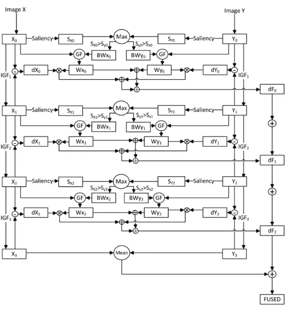
Figure 1 Flow chart of the proposed image fusion scheme.The processing scheme is illustrated for two source imagesXandYand 4 resolution levels (0–3).X0andY0are the original input images, whileXiand
Yirepresent successively lower resolution versions obtained by iterative guided filtering. ‘Saliency’ repre-sents the frequency-tuned saliency transformation, ‘Max’ and ‘Mean’ respectively denote the pointwise maximum and mean operators, ‘(I)GF’ means (Iterative) Guided Filtering, ‘dX,’ ‘dY’ and ‘dF’ are respec-tively the original and fused detail layers, ‘BW’ the binary weight maps, and ‘W’ the smooth weight maps.
PROPOSED METHOD
A flow chart of the proposed multi-scale decomposition fusion scheme is shown inFig. 1. The algorithm consists of the following steps:
1. Iterative guided filtering is applied to decompose the source images into approximate layers (representing large scale variations) and residual layers (containing small scale variations).
3. Binary weighting maps are computed as the pixelwise maximum of the individual source saliency maps.
4. Guided filtering is applied to each binary weighting map with its corresponding source as the guidance image to reduce noise and to restore spatial consistency.
5. The fused image is computed as a weighted recombination of the individual source residual layers.
In a hierarchical framework steps 1–4 are performed at multiple spatial scales. In this paper we used a 4 level decomposition obtained by filtering at three different spatial scales (seeFig. 1).
Figure 2shows the intensified visual (II) and thermal infrared (IR) or near infrared (NIR) images together with the results of the proposed image fusion scheme, for the 12 different scenes that were used in the present study. We will now discuss the proposed fusion scheme in more detail.
Consider two co-registered source imagesX0(x,y) andY0(x,y). The proposed scheme
then applies iterative guided filtering (IGF) to the input images Xi andYi to obtain progressively coarser image representationsXi+1andYi+1(i>0):
IGF(Xi,ri,εi)=Xi+1; i∈ {0,1,2} (12)
where the parametersεiandrirepresent respectively the range and the spatial variances of the guided filter at iteration stepi. In this study the number of iteration steps is set to 4. By letting each finer scale image serve as the approximate layer for the preceding coarser scale image the successive size-selective residual layersdXiare simply obtained by subtraction as follows:
dXi=Xi−Xi+1; i∈ {0,1,2}. (13)
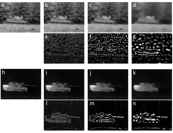
Figure 3shows the approximate and residual layers that are obtained this way for the tank scene (nr 10 inFig. 2). The edge-preserving properties of the iterative guided filter guarantee a graceful decomposition of the source images into details at different spatial scales. The filter size and regularization parameters used in this study are respectively set tori= {5,10,30}andεi= {0.0001,0.01,0.1}fori= {0,1,2}.
Visual saliency refers to the physical, bottom-up distinctness of image details (Fecteau & Munoz, 2006). It is a relative property that depends on the degree to which a detail is visually distinct from its background (Wertheim, 2010). Since saliency quantifies the relative visual importance of image details saliency maps are frequently used in the weighted recombination phase of multi-scale image fusion schemes (Bavirisetti & Dhuli, 2016b;Cui et al., 2015;Gan et al., 2015). Frequency tuned filtering computes bottom-up saliency as local multi-scale luminance contrast (Achanta et al., 2009). The saliency mapS for an imageI is computed as
S(x,y)=Iµ−If(x,y)
(14)
whereIµ is the arithmetic mean image feature vector,If represents a Gaussian blurred version of the original image, using a 5×5 separable binomial kernel,kkis theL2norm
Figure 2 Original input and fused images for all 12 scenes.The intensified visual (II), thermal infrared (IR) or near infrared (NIR: scene 12) source images together with the result of the proposed fusion scheme (F) for each of the 12 scenes used in this study.
Figure 3 Base and detail layers for the tank scene.Original intensified visual (A) and thermal infrared (H) images for scene nr. 10, with their respective base B–D and I–K and detail E–G and L–N layers at suc-cessively lower levels of resolution.
In the proposed fusion scheme we first compute saliency maps SXi andSYi for the
individual source layersXiandYi,i∈ {0,1,2}. Binary weight mapsBWXiandBWYiare then
computed by taking the pixelwise maximum of corresponding saliency mapsSXi andSYi:
BWXi(x,y)=
(
1 if SXi(x,y)>SYi(x,y)
0 otherwise
BWYi(x,y)=
(
1 ifSYi(x,y)>SXi(x,y)
0 otherwise.
(15)
The resulting binary weight maps are noisy and typically not well aligned with object boundaries, which may give rise to artefacts in the final fused image. Spatial consistency is therefore restored through guided filtering (GF) of these binary weight maps with the corresponding source layers as guidance images:
WXi=GF(BWXi,Xi)
WYi=GF(BWYi,Yi).
(16)
Figure 4 Computing smoothed weight maps by guided filtering of binary weight maps.Saliency maps at levels 0, 1 and 2 for respectively the in-tensified visual (A–C) and thermal infrared (D–F) images fromFig. 3. Complementary binary weight maps for both image modalities (G–I and J– L) are obtained with a pointwise maximum operator at corresponding levels. Smooth continuous weight maps (M–O and P–R) are produced by guided filtering of the binary weight maps with their corresponding base layers as guidance images.
continuous weight maps through guided filtering with the corresponding source images as guidance images.Figure 4illustrates the process of computing smoothed weight maps by guided filtering of the binary weight maps resulting from the pointwise maximum of the corresponding source layer saliency maps for the tank scene.
Fused residual layers are then computed as the normalized weighted mean of the corresponding source residual layers:
dFi=
WXi·dXi+WYi·dYi
WXi+WYi
. (17)
The fused imageF is finally obtained by adding the fused residual layers to the average value of the coarsest source layers:
F=X3+Y3
2 +
2
X
i=0
dFi. (18)
By using guided filtering both in the decomposition stage and in the recombination stage, this proposed fusion scheme optimally benefits from both the multi-scale edge-preserving characteristics (in the iterative framework) and the structure restoring capabilities (through guidance by the original source images) of the guided filter. The method is easy to implement and computationally efficient.
METHODS AND MATERIAL
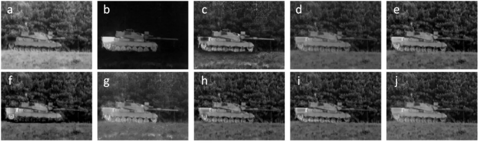
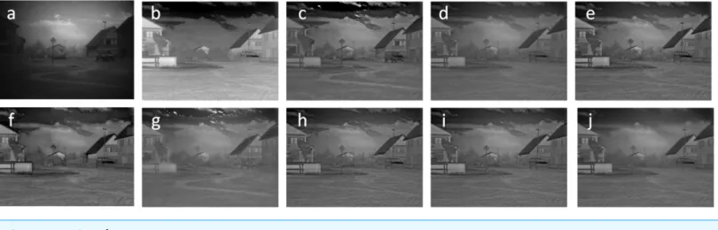
Figure 5 Comparison with existing multiresolution fusion schemes.Original intensified visual (A) and thermal infrared (B) images for scene nr 10, and the fused results obtained with respectively a Contrast Pyramid (C), Gradient Pyramid (D), Laplace Pyramid (E), Morphological Pyramid (F), Ratio Pyramid (G), DWT (H), SIDWT (I), and the proposed method (J), for scene nr. 10.
Test imagery
Figure 2shows the intensified visual (II), thermal infrared (IR) or near infrared (NIR: scene 12) source images together with the result of the proposed fusion scheme (F) for each of the 12 scenes used in this study. The 12 scenes are part of the TNO Image Fusion Dataset (Toet, 2014) with the following identifiers: airplane_in_trees, Barbed_wire_2, Jeep, Kaptein_1123, Marne_07, Marne_11, Marne_15, Reek, tank, Nato_camp_sequence, soldier_behind_smoke, Vlasakkers.
Multi-scale fusion schemes used for comparison
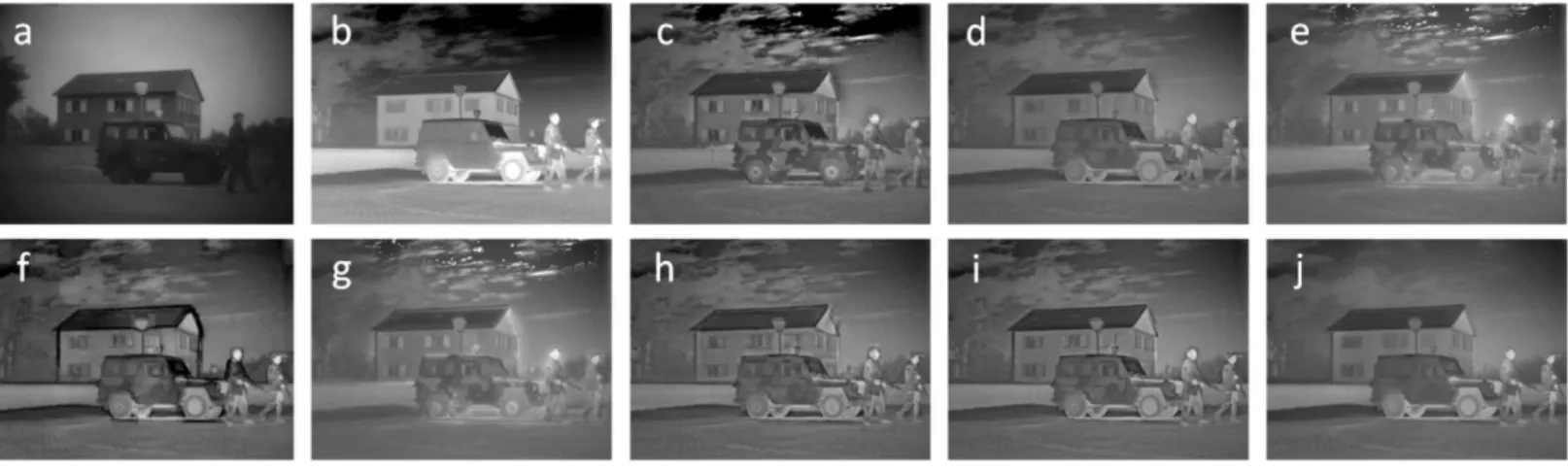
In this study we compare the performance of our image fusion scheme with seven other popular image fusion methods based on multi-scale decomposition including the Laplacian pyramid (Burt & Adelson, 1983), the Ratio of Low-Pass pyramid (Toet, 1989b), the contrast pyramid (Toet, Van Ruyven & Valeton, 1989), the filter-subtract-decimate Laplacian pyramid (Burt, 1988;Burt & Kolczynski, 1993), the gradient pyramid (Burt, 1992;Burt & Kolczynski, 1993), the morphological pyramid (Toet, 1989a), the discrete wavelet transform (Lemeshewsky, 1999;Li, Manjunath & Mitra, 1995;Li, Kwok & Wang, 2002;Scheunders & De Backer, 2001), and a shift invariant extension of the discrete wavelet transform (Lemeshewsky, 1999;Rockinger, 1997;Rockinger, 1999;Rockinger & Fechner, 1998). We used Rockinger’s freely available Matlab image fusion toolbox (www.metapix.de/toolbox.htm) to compute these fusion schemes. To allow a straightforward comparison, the number of scale levels is set to 4 in all methods, and simple averaging is used to compute the approximation of the fused image representation at the coarsest spatial scale.Figures 5–9 show the results of the proposed method together with the results of other seven fusion schemes for some of the scenes used in this study (scenes 2–5 and 10).
Objective evaluation metrics
Figure 6 AsFig. 5, for scene nr. 2.
Figure 7 AsFig. 5, for scene nr. 3.
Figure 9 AsFig. 5, for scene nr. 5.
of time, effort, and equipment required. Also, in most cases, there is only little difference among fusion results. This makes it difficult to subjectively perform the evaluation of fusion results. Therefore, many objective evaluation methods have been developed (for an overview see e.g.,Li, Li & Gong, 2010;Liu et al., 2012). However, so far, there is no universally accepted metric to objectively evaluate the image fusion results. In this paper, we use four frequently applied computational metrics to objectively evaluate and compare the performance of different image fusion methods. The metrics we use are Entropy, the Mean Structural Similarity Index (MSSIM), Normalized Mutual Information (NMI), and Normalized Feature Mutual Information (NFMI). These metrics will be briefly discussed in the following sections.
Entropy
Entropy (E) is a measure of the information content in a fused imageF. Entropy is defined as
EF= − L−1
X
i=0
PF(i)logPF(i) (19)
wherePF(i) indicates the probability that a pixel in the fused imageF has a gray valuei, and the gray values range from 0 toL. The larger the entropy is, the more informative the fused image is. A fused image is more informative than either of its source images when its entropy is higher than the entropy of its source images.
Mean Structural Similarity Index
The Structural Similarity (SSIM: Wang et al., 2004) index is a stabilized version of the Universal Image Quality Index (UIQ:Wang & Bovik, 2002) which can be used to quantify the structural similarity between a source imageAand a fused imageF:
SSIMx,y=
2µxµy+C1
µ2x+µ2y+C1
· 2σxσy+C2 σx2+σy2+C2
· σxy+C3 σxσy+C3
wherexandyrepresent local windows of sizeM×N in respectivelyAandF, and
µx=
1 M×N
M X i=1 N X j=1
x(i,j), µy= 1 M×N
M X i=1 N X j=1
y(i,j) (21)
σx2= 1
M×N M X i=1 N X j=1
(x(i,j)−µx)2, σy2= 1 M×N
M X i=1 N X j=1
(y(i,j)−µy)2 (22)
σxy2 = 1
M×N M X i=1 N X j=1
(x(i,j)−µx)(y(i,j)−µy). (23)
By default, the stabilizing constants are set toC1=(0.01·L)2,C2=(0.03·L)2andC3=C2/2,
whereLis the maximal gray value. The value of SSIM is bounded and ranges between−1 and 1 (it is 1 only when both images are identical). The SSIM is typically computed over a sliding window to compare local patterns of pixel intensities that have been normalized for luminance and contrast. The Mean Structural Similarity (MSSIM) index quantifies the overall similarity between a source imageAand a fused imageF:
MSSIMA,F= 1 Nw
Nw
X
i=1
SSIMxi,yi (24)
whereNw represents the number of local windows of the image. An overall image fusion quality index can then be defined as the mean MSSIM values between each of the source images and the fused result:
MSSIMA,BF =MSSIMA,F+MSSIMB,F
2 (25)
MSSIMA,BF ranges between−1 and 1 (it is 1 only when both images are identical).
Normalized Mutual Information
Mutual Information (MI) measures the amount of information that two images have in common. It can be used to quantify the amount of information from a source image that is transferred to a fused image (Qu, Zhang & Yan, 2002). The mutual information MIAF between a source imageAand a fused imageF is defined as:
MIA,F=
X
i,j
PA,F(i,j)log
PA,F(i,j) PA(i)PF(j)
(26)
wherePA(i) andPF(j) are the probability density functions in the individual images, and PAF(i,j) is the joint probability density function.
The traditional mutual information metric is unstable and may bias the measure towards the source image with the highest entropy. This problem can be resolved by computing the normalized mutual information (NMI) as follows (Hossny, Nahavandi & Creighton, 2008):
NMIA,BF = MIA,F
HA+HF
+ MIB,F
HB+HF
whereHA,HB andHF are the marginal entropy ofA,BandF, and MIA,F and MIB,F represent the mutual information between respectively the source imageAand the fused imageF and between the source imageBand the fused imageF. A higher value of NMI indicates that more information from the source images is transferred to the fused image. The NMI metric varies between 0 and 1.
Normalized Feature Mutual Information
The Feature Mutual Information (FMI) metric calculates the amount of image features that two images have in common (Haghighat & Razian, 2014;Haghighat, Aghagolzadeh & Seyedarabi, 2011). This method outperforms other metrics (e.g., E, NMI) in consistency with the subjective quality measures. Previously proposed MI-based image fusion quality metrics use the image histograms to compute the amount of information a source and fused image have in common (Cvejic, Canagarajah & Bull, 2006;Qu, Zhang & Yan, 2002). However, image histograms contain no information about local image structure (spatial features or local image quality) and only provide statistical measures of the number of pixels in a specific gray-level. However, since meaningful image information is contained in visual features, image fusion quality measures should measure the extent to which these visual features are transferred into the fused image from each of the source images. The Feature Mutual Information (FMI) metric calculates the mutual information between image feature maps (Haghighat & Razian, 2014;Haghighat, Aghagolzadeh & Seyedarabi, 2011). A typical image feature map is for instance the gradient map, which contains information about the pixel neighborhoods, edge strength and directions, texture and contrast. Given two source images asAandBand their fused image asF, the FMI metric first extracts feature maps of the source and fused images using a feature extraction method (e.g., gradient). After feature extraction, the feature imagesA′,B′andF′are normalized to create their marginal probability density functionsPA′,PB′ andPF′. The joint probability
density functions PA′,F′ andPB′,F′ are then estimated from the marginal distributions
using Nelsen’s method (Nelsen, 1987). The algorithm is described in more detail elsewhere (Haghighat, Aghagolzadeh & Seyedarabi, 2011). The FMI metric between a source imageA and a fused imageF is then given by
FMIA,F=MIA′,F′=
X
i,j
PA′,F′(i,j)log PA ′,F′(i,j)
PA′(i)PF′(j) (28)
and the normalized feature mutual information (FMI) can be computed as follows
FMIA,BF = MIA′,F′
HA′+HF′
+ MIB′,F′
HB′+HF′
. (29)
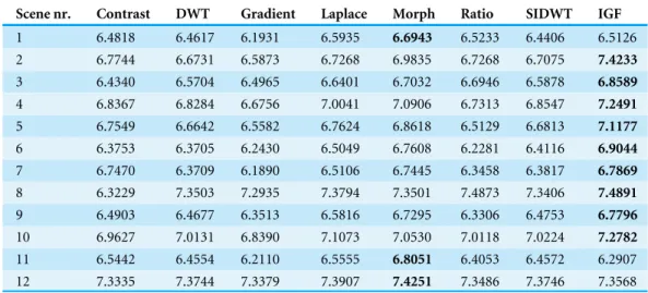
Table 1 Entropy values for each of the methods tested and for all 12 scenes.
Scene nr. Contrast DWT Gradient Laplace Morph Ratio SIDWT IGF
1 6.4818 6.4617 6.1931 6.5935 6.6943 6.5233 6.4406 6.5126
2 6.7744 6.6731 6.5873 6.7268 6.9835 6.7268 6.7075 7.4233
3 6.4340 6.5704 6.4965 6.6401 6.7032 6.6946 6.5878 6.8589
4 6.8367 6.8284 6.6756 7.0041 7.0906 6.7313 6.8547 7.2491
5 6.7549 6.6642 6.5582 6.7624 6.8618 6.5129 6.6813 7.1177
6 6.3753 6.3705 6.2430 6.5049 6.7608 6.2281 6.4116 6.9044
7 6.7470 6.3709 6.1890 6.5106 6.7445 6.3458 6.3817 6.7869
8 6.3229 7.3503 7.2935 7.3794 7.3501 7.4873 7.3406 7.4891
9 6.4903 6.4677 6.3513 6.5816 6.7295 6.3306 6.4753 6.7796
10 6.9627 7.0131 6.8390 7.1073 7.0530 7.0118 7.0224 7.2782
11 6.5442 6.4554 6.2110 6.5555 6.8051 6.4053 6.4572 6.2907
12 7.3335 7.3744 7.3379 7.3907 7.4251 7.3486 7.3746 7.3568
RESULTS
Fusion evaluation
Here we assess the performance of the proposed image fusion scheme on the intensified visual and thermal infrared images for each of the 12 selected scenes, using Entropy, the Mean Structural Similarity Index (MSSIM), Normalized Mutual Information (NMI), and Normalized Feature Mutual Information (NFMI) as the objective performance measures. We also compare the results of the proposed method with those of seven other popular multi-scale fusion schemes.
Table 1lists the entropy of the fused result for the proposed method (IGF) and all seven multi-scale comparison methods (Contrast Pyramid, DWT, Gradient Pyramid, Laplace Pyramid, Morphological Pyramid, Ratio Pyramid, SIDWT). It appears that IGF produces a fused image with the highest entropy for 9 of the 12 test scenes. Note that a larger entropy implies more edge information, but it does not mean that the additional edges are indeed meaningful (they may result from over enhancement or noise). Therefore, we also need to consider structural information metrics.
Table 2shows that IGF outperforms all other multi-scale methods tested here in terms of MSSIM. This means that the mean overall structural similarity between both source images the fused imageF is largest for the proposed method.
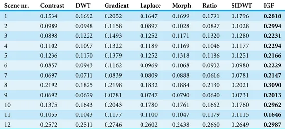
Table 3shows that IGF also outperforms all other multi-scale methods tested here in terms of NMI. This indicates that the proposed IGF fusion scheme transfers more information from the source images to the fused image than any of the other methods.
Table 2 MSSIM values for each of the methods tested and for all 12 scenes.
Scene nr. Contrast DWT Gradient Laplace Morph Ratio SIDWT IGF
1 0.7851 0.7975 0.8326 0.8050 0.7321 0.8054 0.8114 0.8381
2 0.6018 0.6798 0.7130 0.6406 0.6203 0.6406 0.6935 0.7213
3 0.7206 0.7493 0.7849 0.7555 0.6882 0.7468 0.7629 0.7932
4 0.6401 0.6790 0.7162 0.6875 0.6155 0.6668 0.6949 0.7184
5 0.5856 0.6649 0.6938 0.6695 0.6250 0.6270 0.6769 0.7038
6 0.5689 0.6448 0.6755 0.6516 0.5961 0.6099 0.6598 0.6921
7 0.3939 0.5742 0.5994 0.5809 0.5320 0.4490 0.5889 0.6344
8 0.6474 0.6272 0.6630 0.6392 0.5791 0.6291 0.6463 0.6940
9 0.6224 0.6883 0.7224 0.6955 0.6445 0.6718 0.7089 0.7405
10 0.3913 0.5410 0.5715 0.5430 0.4899 0.4331 0.5513 0.5961
11 0.7174 0.7307 0.7754 0.7439 0.6559 0.7419 0.7539 0.7908
12 0.7945 0.8116 0.8466 0.8227 0.7815 0.8106 0.8365 0.8646
Table 3 NMI values for each of the methods tested and for all 12 scenes.
Scene nr. Contrast DWT Gradient Laplace Morph Ratio SIDWT IGF
1 0.1534 0.1692 0.2052 0.1647 0.1699 0.1791 0.1796 0.2818
2 0.0989 0.0948 0.1158 0.0897 0.1028 0.0897 0.1028 0.2994
3 0.0898 0.1222 0.1493 0.1252 0.1171 0.1320 0.1280 0.2231
4 0.1102 0.1097 0.1322 0.1189 0.1169 0.1046 0.1177 0.2294
5 0.1236 0.1170 0.1379 0.1252 0.1318 0.1186 0.1251 0.2166
6 0.0857 0.0943 0.1162 0.0969 0.1068 0.0902 0.0980 0.2229
7 0.0697 0.0711 0.0839 0.0809 0.0888 0.0616 0.0781 0.2147
8 0.2192 0.1825 0.2198 0.1832 0.1884 0.2130 0.2021 0.3090
9 0.0692 0.0679 0.0781 0.0747 0.0790 0.0690 0.0731 0.2013
10 0.1375 0.1643 0.2043 0.1780 0.1761 0.1662 0.1760 0.2962
11 0.1055 0.1043 0.1177 0.1100 0.1047 0.1179 0.1115 0.1646
12 0.2572 0.2511 0.2746 0.2602 0.2438 0.2660 0.2649 0.2987
Summarizing, the proposed IGF fusion scheme appears to outperform the other multi-scale fusion methods investigated here in most of the conditions tested.
Runtime
Table 4 NFMI values for each of the methods tested and for all 12 scenes.
Scene nr. Contrast DWT Gradient Laplace Morph Ratio SIDWT IGF
1 0.4064 0.3812 0.3933 0.3888 0.3252 0.3498 0.4084 0.4008
2 0.4354 0.3876 0.4001 0.3493 0.3432 0.3493 0.4075 0.4383
3 0.4076 0.4081 0.4175 0.4138 0.3758 0.3552 0.4330 0.4454
4 0.4017 0.3913 0.4066 0.4051 0.3655 0.3497 0.4205 0.4490
5 0.4304 0.3971 0.4101 0.4081 0.3758 0.3497 0.4229 0.4580
6 0.4299 0.4074 0.4203 0.4164 0.3832 0.3570 0.4295 0.4609
7 0.5050 0.4383 0.4439 0.4357 0.3942 0.3779 0.4469 0.4286
8 0.4305 0.4074 0.4097 0.4113 0.3806 0.3553 0.4273 0.4325
9 0.4351 0.3959 0.4105 0.3995 0.3658 0.3539 0.4130 0.4370
10 0.4439 0.4251 0.4263 0.4268 0.3863 0.3465 0.4513 0.5045
11 0.3882 0.3798 0.3987 0.3804 0.3131 0.3453 0.4068 0.4206
12 0.4051 0.3725 0.3973 0.3820 0.3449 0.3635 0.4111 0.4257
spatial scale levels i= {0,1,2}. The mean runtime of the proposed fusion method was 0.61±0.05 s.
DISCUSSION AND CONCLUSIONS
We propose a multi-scale image fusion scheme based on guided filtering. Iterative guided filtering is used to decompose the source images into approximation and residual layers. Initial binary weighting maps are computed as the pixelwise maximum of the individual source saliency maps, obtained from frequency tuned filtering. Spatially consistent and smooth weighting maps are then obtained through guided filtering of the binary weighting maps with their corresponding source layers as guidance images. Saliency weighted recombination of the individual source residual layers and the mean of the coarsest scale source layers finally yields the fused image. The proposed multi-scale image fusion scheme achieves spatial consistency by using guided filtering both at the decomposition and at the recombination stage of the multi-scale fusion process. Application to multiband visual (intensified) and thermal infrared imagery demonstrates that the proposed method obtains state-of-the-art performance for the fusion of multispectral nightvision images. The method has a simple implementation and is computationally efficient.
ADDITIONAL INFORMATION AND DECLARATIONS
Funding
Grant Disclosures
The following grant information was disclosed by the author:
Air Force Office of Scientific Research, Air Force Material Command, USAF: FA9550-15-1-0433.
Competing Interests
The author declares there are no competing interests.
Author Contributions
• Alexander Toet conceived and designed the experiments, performed the experiments, analyzed the data, contributed reagents/materials/analysis tools, wrote the paper, prepared figures and/or tables, performed the computation work, reviewed drafts of the paper.
Data Availability
The following information was supplied regarding data availability: Figshare: TNO Image Fusion Dataset
http://dx.doi.org/10.6084/m9.figshare.1008029.
REFERENCES
Achanta R, Hemami S, Estrada F, Süsstrunk S. 2009. Frequency-tuned salient region
de-tection. In: Hemami S, Estrada F, Susstrunk S, eds.IEEE international conference on computer vision and pattern recognition (CVPR2009). Piscataway: IEEE, 1597–1604.
Agarwal J, Bedi SS. 2015.Implementation of hybrid image fusion technique for feature
enhancement in medical diagnosis.Human-centric Computing and Information Sciences5(1):1–17DOI 10.1186/s13673-014-0018-6.
Bavirisetti DP, Dhuli R. 2016a.Fusion of infrared and visible sensor images based
on anisotropic diffusion and Karhunen–Loeve transform.IEEE Sensors Journal
16(1):203–209DOI 10.1109/JSEN.2015.2478655.
Bavirisetti DP, Dhuli R. 2016b.Two-scale image fusion of visible and infrared
images using saliency detection.Infrared Physics and Technology 76:52–64 DOI 10.1016/j.infrared.2016.01.009.
Beyan C, Yigit A, Temizel A. 2011.Fusion of thermal- and visible-band video for
abandoned object detection.Journal of Electronic Imaging 20(033001):1–12 DOI 10.1117/1.3602204.
Bhatnagar G, Wu QMJ. 2011. Human visual system based framework for concealed
weapon detection. In:The 2011 Canadian conference on computer and robot vision (CRV). Piscataway: IEEE, 250–256.
Biswas B, Chakrabarti A, Dey KN. 2015. Spine medical image fusion using wiener
filter in shearlet domain. In:IEEE 2nd international conference on recent trends in information systems (ReTIS 2015). Piscataway: IEEE, 387–392.
Black MJ, Sapiro G, Marimont DH, Heeger D. 1998.Robust anisotropic diffusion.IEEE
Blum RS, Liu Z. 2006.Multi-sensor image fusion and its applications. Boca Raton: CRC Press, Taylor & Francis Group.
Bulanona DM, Burks TF, Alchanatis V. 2009.Image fusion of visible and thermal images
for fruit detection.Biosystems Engineering103(1):12–22 DOI 10.1016/j.biosystemseng.2009.02.009.
Burt PJ. 1988.Smart sensing with a pyramid vision machine.Proceedings IEEE
76(8):1006–1015DOI 10.1109/5.5971.
Burt PJ. 1992. A gradient pyramid basis for pattern-selective image fusion. In:SID
international symposium 1992. Playa del Rey: Society for Information Display, 467–470.
Burt PJ, Adelson EH. 1983.The Laplacian pyramid as a compact image code.IEEE
Transactions on Communications31(4):532–540DOI 10.1109/TCOM.1983.1095851.
Burt PJ, Kolczynski RJ. 1993. Enhanced image capture through fusion. In:Fourth
international conference on computer vision. Piscataway: IEEE Computer Society Press, 173–182.
Cui G, Feng H, Xu Z, Li Q, Chen Y. 2015.Detail preserved fusion of visible and infrared
images using regional saliency extraction and multi-scale image decomposition. Optics Communications341:199–209DOI 10.1016/j.optcom.2014.12.032.
Cvejic N, Canagarajah CN, Bull DR. 2006.Image fusion metric based on
mu-tual information and Tsallis entropy.Electronics Letters42(11):626–627 DOI 10.1049/el:20060693.
Daneshvar S, Ghassemian H. 2010.MRI and PET image fusion by combining IHS and
retina-inspired models.Information Fusion11(2):114–123 DOI 10.1016/j.inffus.2009.05.003.
Farbman Z, Fattal R, Lischinski D, Szeliski R. 2008.Edge-preserving decompositions
for multi-scale tone and detail manipulation.ACM Transactions on Graphics27(3
-Article No. 67):1–10DOI 10.1145/1360612.1360666.
Fecteau JH, Munoz DP. 2006.Salience, relevance, and firing: a priority map for target
selection.Trends in Cognitive Sciences10(8):382–390DOI 10.1016/j.tics.2006.06.011.
Gan W, Wu X, Wu W, Yang X, Ren C, He X, Liu K. 2015.Infrared and visible image
fusion with the use of multi-scale edge-preserving decomposition and guided image filter.Infrared Physics & Technology72:37–51DOI 10.1016/j.infrared.2015.07.003.
Ghassemian H. 2001. A retina based multi-resolution image-fusion. In:IEEE
interna-tional geoscience and remote sensing symposium (IGRSS2001). Piscataway: IEEE, 709–711.
Haghighat MBA, Aghagolzadeh A, Seyedarabi H. 2011.A non-reference image fusion
metric based on mutual information of image features.Computers & Electrical Engineering 37(5):744–756DOI 10.1016/j.compeleceng.2011.07.012.
Haghighat M, Razian MA. 2014.Fast-FMI: non-reference image fusion metric. Piscataway:
IEEE, 1–3.
He K, Sun J, Tang X. 2013.Guided image filtering.IEEE Transactions on Pattern Analysis
Hossny M, Nahavandi S, Creighton D. 2008.Comments on ‘‘Information mea-sure for performance of image fusion’’.Electronics Letters44(18):1066–1067 DOI 10.1049/el:20081754.
Jacobson NP, Gupta MR. 2005.Design goals and solutions for display of hyperspectral
images.IEEE Transactions on Geoscience and Remote Sensing 43(11):2684–2692 DOI 10.1109/TGRS.2005.857623.
Jacobson NP, Gupta MR, Cole JB. 2007.Linear fusion of image sets for display.IEEE
Transactions on Geoscience and Remote Sensing 45(10):3277–3288 DOI 10.1109/TGRS.2007.903598.
Jiang D, Zhuang D, Huan Y, Fu J. 2011. Survey of multispectral image fusion techniques
in remote sensing applications. In: Zheng Y, ed.Image fusion and its applications. Rijeka, Croatia: InTech Open, 1–22.
Kong SG, Heo J, Boughorbel F, Zheng Y, Abidi BR, Koschan A, Yi M, Abidi MA.
2007.Multiscale fusion of visible and thermal IR images for
illumination-invariant face recognition.International Journal of Computer Vision71(2):215–233 DOI 10.1007/s11263-006-6655-0.
Kong W, Wang B, Lei Y. 2015.Technique for infrared and visible image fusion based
on non-subsampled shearlet transform & spiking cortical model.Infrared Physics & Technology71:87–98DOI 10.1016/j.infrared.2015.02.008.
Kumar BKS. 2013.Image fusion based on pixel significance using cross bilateral filter.
Signal, Image and Video Processing 9(5):1193–1204DOI 10.1007/s11760-013-0556-9.
Lemeshewsky GP. 1999.Park SJ, Juday RD, eds.Multispectral multisensor image
fusion using wavelet transforms. Bellingham: The International Society for Optical Engineering, 214–222.
Lepley JJ, Averill MT. 2011. Detection of buried mines and explosive objects using
dual-band thermal imagery. In: Harmon RS, Holloway JH, Broach JT, eds.Detection and sensing of mines, explosive objects, and obscured targets XVI, Vol. SPIE-8017. Bellingham: The International Society for Optical Engineering, 80171V80171-80112.
Li S, Kang X, Hu J. 2013.Image fusion with guided filtering.IEEE Transactions on Image
Processing22(7):2864–2875DOI 10.1109/TIP.2013.2244222.
Li S, Kwok JT, Wang Y. 2002.Using the discrete wavelet frame transform to merge
Landsat TM and SPOT panchromatic images.Information Fusion3(1):17–23 DOI 10.1016/S1566-2535(01)00037-9.
Li S, Li Z, Gong J. 2010.Multivariate statistical analysis of measures for assessing the
quality of image fusion.International Journal of Image and Data Fusion1(1):47–66 DOI 10.1080/19479830903562009.
Li H, Manjunath BS, Mitra SK. 1995.Multisensor image fusion using the wavelet
transform.Computer Vision, Graphics and Image Processing: Graphical Models and Image Processing 57(3):235–245.
Liu Z, Blasch EP, Xue Z, Zhao J, Laganière R, Wu W. 2012.Objective assessment of
multiresolution image fusion algorithms for context enhancement in night vision: a comparative study.IEEE Transactions on Pattern Analysis and Machine Intelligence
Liu X, Mei W, Du H, Bei J. 2016.A novel image fusion algorithm based on nonsubsam-pled shearlet transform and morphological component analysis.Signal, Image and Video Processing 10(5):959–966DOI 10.1007/s11760-015-0846-5.
Liu Z, Xue Z, Blum RS, Laganiëre R. 2006.Concealed weapon detection and
visu-alization in a synthesized image.Pattern Analysis & Applications8(4):375–389 DOI 10.1007/s10044-005-0020-8.
Motamed C, Lherbier R, Hamad D. 2005. A multi-sensor validation approach for
human activity monitoring. In:7th international conference on information fusion (Information Fusion 2005). Piscataway: IEEE.
Nelsen RB. 1987.Discrete bivariate distributions with given marginals and
correla-tion.Communications in Statistics—Simulation and Computation16(1):199–208 DOI 10.1080/03610918708812585.
O’Brien MA, Irvine JM. 2004.Information fusion for feature extraction and the
develop-ment of geospatial information. In:7th international conference on information fusion. ISIF, 976–982.
Perona P, Malik J. 1990.Scale-space and edge detection using anisotropic diffusion.
IEEE Transactions on Pattern Analysis and Machine Intelligence12(7):629–639 DOI 10.1109/34.56205.
Petrovic VS, Xydeas CS. 2003.Sensor noise effects on signal-level image fusion
perfor-mance.Information Fusion4(3):167–183DOI 10.1016/S1566-2535(03)00035-6.
Petschnigg G, Agrawala M, Hoppe H, Szeliski R, Cohen M, Toyama K. 2004.Digital
photography with flash and no-flash image pairs. New York: ACM Press, 664–672.
Qu GH, Zhang DL, Yan PF. 2002.Information measure for performance of image
fusion.Electronics Letters38(7):313–315DOI 10.1049/el:20020212.
Rockinger O. 1997. Image sequence fusion using a shift-invariant wavelet transform.
In:IEEE international conference on image processing, Vol. III. Piscataway: IEEE, 288–291.
Rockinger O. 1999.Multiresolution-Verfahren zur Fusion dynamischer Bildfolge. PhD
Thesis, Technische Universität Berlin.
Rockinger O, Fechner T. 1998. Pixel-level image fusion: the case of image sequences.
In: Kadar I, ed.Signal processing, sensor fusion, and target recognition VII, vol. SPIE-3374. Bellingham: The International Society for Optical Engineering, 378–388.
Scheunders P, De Backer S. 2001.Fusion and merging of multispectral images
us-ing multiscale fundamental forms.Journal of the Optical Society of America A
18(10):2468–2477DOI 10.1364/JOSAA.18.002468.
Shah P, Reddy BCS, Merchant S, Desai U. 2013.Context enhancement to reveal
a camouflaged target and to assist target localization by fusion of multispec-tral surveillance videos.Signal, Image and Video Processing 7(3):537–552 DOI 10.1007/s11760-011-0257-1.
Singh R, Khare A. 2014.Fusion of multimodal medical images using Daubechies
complex wavelet transform—a multiresolution approach.Information Fusion
Singh R, Vatsa M, Noore A. 2008.Integrated multilevel image fusion and match score fusion of visible and infrared face images for robust face recognition.Pattern Recognition41(3):880–893DOI 10.1016/j.patcog.2007.06.022.
Tao C, Junping Z, Ye Z. 2005. Remote sensing image fusion based on ridgelet transform.
In:2005 IEEE international geoscience and remote sensing symposium (IGARSS’05), Vol. 2. Piscataway: IEEE, 1150–1153.
Tian YP, Zhou KY, Feng X, Yu SL, Liang H, Liang B. 2009.Image fusion for infrared
thermography and inspection of pressure vessel.Journal of Pressure Vessel Technology
131(2 - article no. 021502):1–5DOI 10.1115/1.3066801.
Toet A. 1989a.A morphological pyramidal image decomposition.Pattern Recognition
Letters9(4):255–261DOI 10.1016/0167-8655(89)90004-4.
Toet A. 1989b.Image fusion by a ratio of low-pass pyramid.Pattern Recognition Letters
9(4):245–253DOI 10.1016/0167-8655(89)90003-2.
Toet A. 2003. Color image fusion for concealed weapon detection. In: Carapezza EM, ed.
Sensors, and command, control, communications, and intelligence (C3I) technologies for homeland defense and law enforcement II, Vol. SPIE-5071. Bellingham: SPIE, 372–379.
Toet A. 2011.Computational versus psychophysical image saliency: a comparative
evaluation study.IEEE Transactions on Pattern Analysis and Machine Intelligence
33(11):2131–2146DOI 10.1109/TPAMI.2011.53.
Toet A. 2014.TNO Image fusion dataset.FigshareDOI 10.6084/m9.figshare.1008029.
Toet A, IJspeert I, Waxman AM, Aguilar M. 1997.Fusion of visible and thermal imagery
improves situational awareness.Displays18(2):85–95 DOI 10.1016/S0141-9382(97)00014-0.
Toet A, Van Ruyven LJ, Valeton JM. 1989.Merging thermal and visual images by a
contrast pyramid.Optical Engineering 28(7):789–792 DOI 10.1117/12.7977034.
Tomasi C, Manduchi R. 1998. Bilateral filtering for gray and color images. In:IEEE sixth
international conference on computer vision. Piscataway: IEEE, 839–846.
Wang Z, Bovik AC. 2002.A universal image quality index.IEEE Signal Processing Letters
9(3):81–84DOI 10.1109/97.995823.
Wang Z, Bovik AC, Sheikh HR, Simoncelli EP. 2004.Image quality assessment: from
error visibility to structural similarity.IEEE Transactions on Image Processing
13(4):600–612DOI 10.1109/TIP.2003.819861.
Wang L, Li B, Tian LF. 2014.Multi-modal medical image fusion using the inter-scale
and intra-scale dependencies between image shift-invariant shearlet coefficients. Information Fusion19:20–28DOI 10.1016/j.inffus.2012.03.002.
Wertheim AH. 2010.Visual conspicuity: a new simple standard, its reliability, validity
and applicability.Ergonomics53(3):421–442DOI 10.1080/00140130903483705.
Xue Z, Blum RS. 2003. Concealed weapon detection using color image fusion. In:Sixth
Xue Z, Blum RS, Li Y. 2002. Fusion of visual and IR images for concealed weapon detection. In:Fifth international conference on information fusion, Vol. 2. Piscataway: IEEE, 1198–1205.
Yajie W, Mowu L. 2009. Image fusion based concealed weapon detection. In:
Inter-national conference on computational intelligence and software engineering 2009 (CiSE2009). Piscataway: IEEE, 1–4.
Yang W, Liu J-R. 2013. Research and development of medical image fusion. In:2013
IEEE international conference on medical imaging physics and engineering (ICMIPE). Piscataway: IEEE, 307–309.
Yang S, Wang M, Jiao L, Wu R, Wang Z. 2010.Image fusion based on a new contourlet
packet.Information Fusion11(2):78–84DOI 10.1016/j.inffus.2009.05.001.
Yong J, Minghui W. 2014.Image fusion using multiscale edge-preserving
decompo-sition based on weighted least squares filter.IET Image Processing 8(3):183–190 DOI 10.1049/iet-ipr.2013.0429.
Zhang B, Lu X, Pei H, Zhao Y. 2015.A fusion algorithm for infrared and visible images
based on saliency analysis and non-subsampled Shearlet transform.Infrared Physics & Technology73:286–297DOI 10.1016/j.infrared.2015.10.004.
Zhang Q, Shen X, Xu L, Jia J. 2014. Rolling guidance filter. In: Fleet D, Pajdla T, Schiele
B, Tuytelaars T, eds.13th European conference on computer vision (ECCV2014), Vol. III. Berlin Heidelberg: Springer International Publishing, 815–830.
Zhao J, Feng H, Xu Z, Li Q, Liu T. 2013.Detail enhanced multi-source fusion using
visual weight map extraction based on multi scale edge preserving decomposition. Optics Communications287:45–52DOI 10.1016/j.optcom.2012.08.070.
Zhu Z, Huang TS. 2007.Multimodal surveillance: sensors, algorithms and systems.
Norwood: Artech House Publishers.
Zitová B, Beneš M, Blažek J. 2011. Image fusion for art analysis. In:Computer vision and
image analysis of art II, Vol. SPIE-7869. Bellingham: The International Society for Optical Engineering, 7869081–7869089.
Zou X, Bhanu B. 2005. Tracking humans using multi-modal fusion. In:2nd joint IEEE