www.atmos-chem-phys.net/17/745/2017/ doi:10.5194/acp-17-745-2017
© Author(s) 2017. CC Attribution 3.0 License.
Characterisation of boundary layer turbulent processes
by the Raman lidar BASIL in the frame of HD(CP)
2
Observational Prototype Experiment
Paolo Di Girolamo1, Marco Cacciani2, Donato Summa1, Andrea Scoccione2, Benedetto De Rosa1, Andreas Behrendt3, and Volker Wulfmeyer3
1Scuola di Ingegneria, Università degli Studi della Basilicata, Viale dell’Ateneo Lucano n. 10, 85100 Potenza, Italy 2Dipartimento di Fisica, Università di Roma “La Sapienza”, Piazzale Aldo Moro, n. 2, 00100 Rome, Italy
3Institut für Physik und Meteorologie, Universität Hohenheim, Garbenstraße 30, D-70599 Stuttgart, Germany Correspondence to:Paolo Di Girolamo ([email protected])
Received: 30 June 2016 – Published in Atmos. Chem. Phys. Discuss.: 7 July 2016 Revised: 27 October 2016 – Accepted: 7 November 2016 – Published: 17 January 2017
Abstract. Measurements carried out by the University of Basilicata Raman lidar system (BASIL) are reported to demonstrate the capability of this instrument to characterise turbulent processes within the convective boundary layer (CBL). In order to resolve the vertical profiles of turbu-lent variables, high-resolution water vapour and temperature measurements, with a temporal resolution of 10 s and verti-cal resolutions of 90 and 30 m, respectively, are considered. Measurements of higher-order moments of the turbulent fluc-tuations of water vapour mixing ratio and temperature are obtained based on the application of autocovariance analy-ses to the water vapour mixing ratio and temperature time series. The algorithms are applied to a case study (11:30– 13:30 UTC, 20 April 2013) from the High Definition Clouds and Precipitation for Climate Prediction (HD(CP)2) Obser-vational Prototype Experiment (HOPE), held in western Ger-many in the spring 2013. A new correction scheme for the removal of the elastic signal crosstalk into the low quantum number rotational Raman signal is applied. The noise errors are small enough to derive up to fourth-order moments for both water vapour mixing ratio and temperature fluctuations. To the best of our knowledge, BASIL is the first Raman li-dar with a demonstrated capability to simultaneously retrieve daytime profiles of water vapour turbulent fluctuations up to the fourth order throughout the atmospheric CBL. This is combined with the capability of measuring daytime profiles of temperature fluctuations up to the fourth order. These mea-surements, in combination with measurements from other
li-dar and in situ systems, are important for verifying and pos-sibly improving turbulence and convection parameterisation in weather and climate models at different scales down to the grey zone (grid increment∼1 km; Wulfmeyer et al., 2016).
For the considered case study, which represents a well-mixed and quasi-stationary CBL, the mean boundary layer height is found to be 1290±75 m above ground level (a.g.l.). Values of the integral scale for water vapour and temperature fluctuations at the top of the CBL are in the range of 70–125 and 75–225 s, respectively; these values are much larger than the temporal resolution of the measurements (10 s), which testifies that the temporal resolution considered for the mea-surements is sufficiently high to resolve turbulent processes down to the inertial subrange and, consequently, to resolve the major part of the turbulent fluctuations. Peak values of all moments are found in the interfacial layer in the proximity of the top of the CBL. Specifically, water vapour and tempera-ture second-order moments (variance) have maximum values of 0.29 g2kg−2and 0.26 K2; water vapour and temperature third-order moments have peak values of 0.156 g3kg−3and
−0.067 K3, while water vapour and temperature fourth-order
moments have maximum values of 0.28 g4kg−4and 0.24 K4.
confidence in the possibility of using these measurements for turbulence parameterisation in weather and climate models.
In the determination of the temperature profiles, particular care was dedicated to minimise potential effects associated with elastic signal crosstalk on the rotational Raman signals. For this purpose, a specific algorithm was defined and tested to identify and remove the elastic signal crosstalk and to as-sess the residual systematic uncertainty affecting tempera-ture measurements after correction. The application of this approach confirms that, for the present Raman lidar system, the crosstalk factor remains constant with time; consequently an appropriate assessment of its constant value allows for a complete removal of the leaking elastic signal from the rota-tional Raman lidar signals at any time (with a residual error on temperature measurements after correction not exceeding 0.18 K).
1 Introduction
Water vapour and temperature are key meteorological vari-ables which play a major role in the definition of the thermo-dynamic state of the atmosphere (Wulfmeyer et al., 2015). This is particularly true in the convective boundary layer (CBL), which is an unstable stratified boundary layer that develops in the lower troposphere during the day, dominated by buoyant turbulence generation as a result of strong sur-face solar heating (Garratt, 1992). Entrainment processes at the top of the CBL are controlled by temperature (capping) inversion in the interfacial layer, ultimately influencing the vertical transport of humidity in the free troposphere (Mahrt, 1991; Sorbjan, 1996; Sullivan et al., 1998; Wulfmeyer et al., 2016). Accurate measurements of water vapour and tempera-ture from the surface to the entrainment zone at the top of the CBL are, therefore, essential for improving weather forecast-ing (Dierer et al., 2009), reanalyses (Bengtsson et al., 2004) and regional climate simulations (Milovac et al., 2016).
Measurements of higher-order moments of moisture and temperature fluctuations provide unique and essential infor-mation for the characterisation of turbulent processes within the convective boundary layer (CBL). Water vapour and temperature variances are key variables in turbulence, con-vection and cloud parameterisations considered in weather and climate models (e.g. Stull, 1988; Berg and Stull, 2005; Gustafson and Berg, 2007). Within the CBL, water vapour variance increases with height, achieving a maximum at the top of the CBL due to the mixing of moist air in the up-draughts with drier air from above the CBL (Wulfmeyer 1999a, b; Kiemle et al., 2007). The water vapour variance profile can also be used to estimate the CBL height and characterise its internal structure by exploiting the tracing capabilities of atmospheric water vapour (among others, Wulfmeyer et al., 2010; Turner et al., 2014a, b). Further-more, water vapour skewness and kurtosis are found to be
characterised by an appreciable vertical variability within the CBL, which changes patterns during the different phases of the CBL evolution (Couvreaux et al., 2005, 2007).
Atmospheric turbulent processes within the CBL have been studied for decades based on the use of in situ sensors (among others, Lenschow and Kristensen, 1985; Kalthoff et al., 2011). However, lidar systems, on the basis of their capa-bility to provide high spatial and temporal resolution and ac-curate measurements of atmospheric water vapour and tem-perature, have nowadays reached the level of maturity needed to investigate the relevant atmospheric processes and enable measurements of turbulent variables within the CBL (among others, Eberhard et at., 1989; Frehlich and Cornman, 2002). The major advantage of the lidar techniques is represented by their capability to characterise turbulent variables from the proximity of the surface up to the interfacial layer and above. Additionally, lidar systems can be operated from different platforms and, when applied from ground-based platforms, can provide excellent long-term statistics. This is also neces-sary for reducing sampling errors, which are usually larger for ground-based than for airborne measurements.
for the considered case study were too large to derive fourth-order moments with sufficient accuracy. Thus, to the best of our knowledge, BASIL is the first Raman lidar with a demon-strated capability to accurately measure simultaneous day-time profiles of water vapour and temperature turbulent fluc-tuations up to the fourth order throughout the atmospheric CBL. The main aim of this paper is to provide a detailed char-acterisation of the performances of the Raman lidar BASIL and demonstrate that profiles of turbulent variables can be determined throughout the CBL with sufficient accuracy. For this purpose measurements from the High Definition Clouds and Precipitation for Climate Prediction (HD(CP)2) Obser-vational Prototype Experiment (HOPE), held in western Ger-many in spring 2013, are considered.
The paper outline is the following. Section 2 provides a description of the experimental set-up, with details on the data processing and the error analyses; this section also de-scribes the correction scheme considered for removing the elastic signal crosstalk from the low quantum number rota-tional Raman signal and the uncertainties associated with this approach. Section 3 provides a brief overview of the HOPE field campaign and illustrates the criteria considered for the selection of the case study; this section also illustrates the time–height cross sections of the water vapour mixing ratio and temperature data considered for the turbulence analysis, providing remarks on the meteorological conditions occur-ring duoccur-ring this period. Section 4 provides a brief descrip-tion of the methodology considered for the turbulence anal-ysis and illustrates the results achieved in terms of vertical profiles of turbulent variables. Finally, Sect. 5 summarises all results and provides some indications for possible future work.
2 Experimental set-up
2.1 System set-up and derivation of mixing-ratio and temperature profiles
Prior to HOPE, the University of Basilicata Raman lidar system (BASIL) underwent a substantial upgrade aimed to improve its overall performances in terms of measurement precision and vertical and temporal resolution. These set-up modifications will be described in a separate forthcoming pa-per (Di Girolamo et al., 2016b). BASIL is a ground-based Raman lidar hosted in a transportable seatainer. The major feature of BASIL is represented by its capability to perform high-resolution and accurate measurements of the vertical profiles of atmospheric temperature and water vapour, both in the daytime and at night-time, based on the application of the rotational and vibrational Raman lidar techniques in the UV (Di Girolamo et al., 2004, 2006, 2009a, 2016a, Bhawar et al., 2011). Besides temperature and water vapour, BASIL is also capable of providing measurements of the vertical pro-files of particle backscatter at 354.7, 532 and 1064 nm,
par-ticle extinction at 354.7 and 532 nm and parpar-ticle depolarisa-tion at 354.7 and 532 nm (Griaznov et al., 2007; Di Girolamo et al., 2009b, 2012a, b). BASIL is built around a Nd:YAG laser source, equipped with second and third harmonic gen-eration crystals, capable of emitting pulses at 354.7, 532 and 1064 nm, which are simultaneously transmitted in the atmosphere along the zenith. The receiver includes a large-aperture telescope in Newtonian configuration, with a 45 cm diameter primary mirror and a focal length of 2.1 m, and two small-aperture telescopes (50 mm diameter lenses). The ra-diation collected by the large-aperture telescope is split into eight portions by means of dichroic or partially reflecting mirrors. Specifically, two portions are fed into the detection channels used for temperature measurements (at 354.3 and 352.9 nm for the low and high quantum number rotational Raman signals,PLoJ(z)andPHiJ(z)), while two other
por-tions are sent to the water vapour (at 407.5 nm) and molec-ular nitrogen Raman channels (at 386.7 nm); corresponding signals are PH2O(z) andPN2(z) in the following. Another two portions of the collected radiation are fed into the 354.7 and 532 nm elastic channels. A fraction of the signal entering the 354.7 nm channel is split into two additional portions to allow the detection of the parallel and cross-polarised elas-tic signals, which are used for the determination parelas-ticle de-polarisation. Signal selection is performed by means of nar-rowband interference filters, the specifications of which were defined in Di Girolamo et al. (2004, 2009a).
The water vapour mixing ratiomcan be obtained from the power ratio of water vapour to molecular nitrogen vibrational Raman signals m (z)=K (z)× PH2O(z) /PN2(z)
, where
K(z)=c·f (z)is a calibration factor obtained by multiply-ing several dependent correction terms and a height-independent calibration term,c(e.g. Whiteman, 2003). The height-dependent correction terms,f (z), included inK(z), are a differential transmission term, accounting for the dif-ferent atmospheric transmission by molecules and aerosols at the two wavelengths corresponding to the water vapour and molecular nitrogen Raman signals, and a term asso-ciated with the use of narrowband interference filters and the consequent temperature dependence of H2O and N2
Ra-man scattering signals selected by these filters. The height-independent calibration factorcis finally obtained from the multiplication of the above-mentioned signal ratio by the height-dependent correction terms,f (z), and the comparison of this quantity with simultaneous and co-located mixing ra-tio measurements from different sensors (e.g. from radioson-des, microwave radiometers, GPS tomography).
Based on the application of the pure rotational Raman li-dar technique, atmospheric temperature is obtained from the power ratio of high-to-low quantum number rotational Ra-man signalsQ(z)through the application of the analytical expression:
withαandβbeing two calibration constants. Thus we gain the following:
T (z)= α
ln[Q(z)] −β. (2)
These two calibration constants can be determined through the comparison of the lidar signal ratio with simultane-ous and co-located temperature measurements from differ-ent sensors (e.g. from radiosondes, microwave radiometers). The above-considered analytical expression relatingQ(z)to
T (z) is not the only possible expression, but it is probably the simplest and implies the smallest number of calibration constants. Other more complex analytical expressions have been considered in literature (Behrendt and Reichardt, 2000; Di Girolamo et al., 2004; Behrendt et al., 2015). However, the systematic error associated with assuming the above-calibration function to be valid for a large portion of the rota-tional Raman spectrum is found to have a typical amplitude of 0.2 K, which is not relevant for the purposes of the present study (see Wulfmeyer et al., 2016 for an assessment of the effects of systematic errors on turbulence measurements).
During HOPE, water vapour mixing ratio and tempera-ture measurements by BASIL were both calibrated based on a comparison with simultaneous radiosondes, which were launched from the nearby supersite UHOH-KIT, located in Hambach, approx. 4 km E–SE. All clear-sky radiosonde launches coincident with lidar operation (60 in total) were considered, thus determining 60 distinct values for each cal-ibration coefficient. A mean value for each calcal-ibration co-efficient was then estimated and used throughout the HOPE period. The comparisons were carried out in a vertical region with an extent of 1 km located above the boundary layer. This selection allows for minimising the air mass differences re-lated to the physical distance between the lidar and the ra-diosonde. The variability of the calibration coefficients was found to be very limited throughout the duration of the filed campaign, with single calibration values showing very small deviations from the mean values. For example, concerning water vapour measurements, the standard deviation of single calibration values from the mean calibration coefficient was found to not exceed 5 %.
As specified above, BASIL underwent an upgrade before HOPE which allowed for obtaining a substantial improve-ment of the overall performances in terms of both measure-ment precision and vertical and temporal resolution. The up-grade included a modification of the optical layout of the Nd:YAG laser source, which allowed a 65 % increase of the emitted power in the UV to be achieved (from an original value of 6 W, single pulse energy of 300 mJ at 20 Hz, to a final value of 10 W, with a single pulse energy of 500 mJ at 20 Hz). The upgrade also included the implementation of a new sampling system (with double signal acquisition mode, i.e. both analogue and digital) in some of the measurement channels allowing us to acquire daytime and night-time lidar signals with a maximum vertical and temporal resolution of
0 500 1000 1500 2000 2500 3000
0,01 0,1 1 10
T=5 mins, z=150 m N oise variance Poisson statistics
x (g kg )
H2O
He
ight
a
.g.l
. (m
)
T=10 s, z=90 m N oise variance Poisson statistics
0 500 1000 1500 2000 2500 3000
1 10 100 1000
T=5 mins, z=150 m N oise variance Poisson statistics
x
H2O
/x
H2O
(%)
He
ight
a
.g.l
. (m
)
T=10 s, z=90 m N oise variance Poisson statistics
0 500 1000 1500 2000 2500 3000
0,01 0,1 1 10
T=5 min, z=150 m N oise variance Poisson statistics
T (K)
Hei
g
ht
a.g.l
. (m)
T=10 s, z=90 m N oise variance Poisson statistics
(a)
(b)
(c) –1
7.5 m and 1–10 s, respectively. In signal preprocessing, four adjacent data points are binned together to reduce the statis-tical fluctuations of the signals, increasing the verstatis-tical step between adjacent data points to 30 m.
2.2 Determination of noise errors
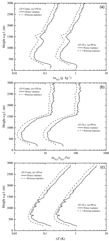
In order to characterise the quality of water vapour mixing ratio and temperature measurements, an accurate assessment of noise error is necessary. Noise error is quantified as the root-square of the noise variance (i.e. the noise standard de-viation). Profiles of noise error affecting water vapour mixing ratio and temperature measurements are illustrated in Fig. 1. Specifically, Fig. 1a illustrates the water vapour mixing ratio absolute error (expressed in g kg−1), Fig. 1b illustrates the
water vapour mixing ratio relative error (expressed in %), while Fig. 1c illustrates the temperature absolute error (ex-pressed in K). The figure shows the noise error profiles esti-mated based on the application of the autocovariance method (described in detail in Sect. 4.1). More specifically, noise er-ror assessments have been performed considering two op-tions for temporal and vertical resolution: a higher-resolution configuration, with a temporal resolution of 10 s and a verti-cal resolution of 90 and 30 m for water vapour mixing ratio and temperature, respectively (this is the selection consid-ered for the turbulence measurements) and a lower-resolution configuration, with a temporal resolution of 150 m and a vertical resolution of 5 min, which is the selection consid-ered for the data set generated and uploaded to the HOPE archive (see Sect. 6, primarily used for verification purposes, process studies and data assimilation). For the first selec-tion, the statistical error affecting water vapour mixing ra-tio measurements is smaller than 0.6 g kg−1(or 50 %) up to
1.4 km, while the statistical error affecting temperature mea-surements is smaller than 1 K up to 1.8 km. For the second selection, the statistical error affecting water vapour mixing ratio measurements is smaller than 0.1 g kg−1(or 15 %) up to 1.8 km, while the statistical error affecting temperature mea-surements is smaller than 0.8 K up to 3 km. The above-listed performances of BASIL in terms of water vapour mixing ra-tio measurements are comparable with those reported for the ARM Raman lidar (Wulfmeyer et al., 2010, also 0.6 g kg−1 at 1.4 km), considering the same temporal and vertical res-olution. The same is true for the above-listed performances of BASIL in terms of temperature measurements, which in-dicate statistical uncertainties with values close to those re-ported for the ARM Raman lidar (Newsom et al., 2013). The above-quantified errors are used to derive – by means of error propagation – the noise error profiles of the higher-order mo-ments. An overview of these equations is given in Wulfmeyer et al. (2016).
Water vapour mixing ratio and temperature profiles can be derived with different vertical and temporal resolutions de-pending on the considered application. Vertical and temporal resolutions can be traded-off with measurement precision,
0 3000 6000 9000 12 000 15 000
1 10 100 1000 10000
0,00 0,05 0,10
R(z)/T (K-1)
Photon number
H
eig
h
t a
.g
.l.
(
m
)
P355(z) PH
2O
(z) PN
2
(z) PHiJ(z) PLoJ(z)
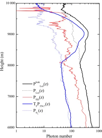
Figure 2. (a)The mean photon numbers (10 s average) for the con-sidered signals, i.e. the water vapour and molecular nitrogen vi-brational Raman signals,PH2O(z) andPN2(z), the 355 nm elas-tic signal,P355(z)and the pure-rotational Raman signals,PLoJ(z) andPHiJ(z);(b)temperature sensitivity of RRL measurement tech-nique.∂R (z) /∂T.
with random error affecting water vapour mixing ratio and temperature measurements being inversely proportional to the square root of both vertical and temporal resolution. Con-sequently, the consideration of the high temporal and vertical resolutions (10 s, 30–90 m, respectively) needed for the char-acterisation of turbulence processes translates into a lower measurement precision (and consequently a larger statistical error). As a result of this, the corresponding statistical error affecting daytime water vapour mixing ratio and temperature measurements is smaller than 100 % and 1 K, respectively, up to 2 km (Fig. 1), these performances being well suited for lidar measurements finalised to the characterisation of turbu-lent variables.
vapour mixing ratio and temperature measurements through Poisson statistics, it is necessary to first apply Poisson statis-tics to the photon counts of the individual lidar signals con-tributing to the measurements and then, through error prop-agation, compute the overall error affecting the measured at-mospheric variables. The error propagation expression is dif-ferent for water vapour mixing ratio and temperature mea-surements as are the analytical expressions relating the in-dividual signals to the two measured parameters. For water vapour mixing ratio measurements the application of error propagation yields the following expression (Di Girolamo et al., 2009a):
1xH2O(z) xH2O(z)
=
s
PH2O(z)+bkH2O PH2
2O(z)
+PN2(z)+bkN2
PN2 2(z)
, (3)
where the terms bkH2O and bkN2 represent the sky back-ground signal (primarily associated with solar irradiance) collected in the water vapour and molecular nitrogen chan-nels, respectively. Equation (3) provides the relative statisti-cal error (in percentage if multiplied for 100), while the ab-solute statistical error can be obtained by multiplying Eq. (3) for xH2O(z). The mean photon numbers for the 10 s water vapour and molecular nitrogen vibrational Raman signals,
PH2O(z)andPN2(z), displayed in Fig. 2, are found to vary featuring a maximum around 800 m of approx. 1500 and 12 000 counts and progressively decreasing down to 0 and approx. 20 counts around 10 km (after background subtrac-tion). Here the mean photon number profile is intended as the average of all 10 s signal profiles collected over the pe-riod 11:30–13:30 UT on 20 April 2013. Figure 2 also shows the mean photon number for the 10 s 354.7 nm elastic sig-nal,P354.7(z), which has a maximum of approx. 2200 counts
around 800 m and progressively decreases to 2 counts around 10 km.
For temperature measurements, the application of error propagation yields the expression (Behrendt et al., 2002, 2015; Di Girolamo et al., 2006, 2009a):
1T (z)=∂T (z)
∂R R (z)
s
PLoJ(z)+bkLoJ
PLoJ2 (z) +
PHiJ(z)+bkHiJ
PHiJ2 (z) , (4) where the terms bkLoJ and bkHiJ represent the sky
back-ground signal collected in the low- and high-J-rotational Ra-man channels, respectively. The quantity∂T (z) /∂Rcan be estimated based on the application of the calibration proce-dure mentioned above. The mean photon numbers for the 10 s low and high quantum number rotational Raman sig-nals,PLoJ(z)andPHiJ(z), also displayed in Fig. 2, are found
to vary, featuring a maximum of approx. 4500 and 3500 counts at 800 m, and progressively decreasing down to 8 and 4 counts around 10 km. Figure 2 also shows the temperature sensitivity of the RRL measurement technique, i.e. the quan-tity∂R (z) /∂T, which is found to vary between 0.06 K−1at surface level and approx. 0.03 K−1at 10 km, and the power
ratio of high-to-low quantum number rotational Raman sig-nals,R(z), which is found to vary between approx. 0.8 at surface level and approx. 0.3 at 10 km. The large values of the measurement sensitivity (∂R (z) /∂T ) contribute to the small random errors affecting the reported temperature mea-surements.
The terms bkH2Oand bkN2 in Eq. (3) and the terms bkLoJ and bkHiJ in Eq. (4) can be determined from the
photon-counting signals at very high heights. In fact, this portion of the signals is characterised by negligible contribution from laser backscatter photons and is typically attributable to sky background radiation and intrinsic detector noise, with the former quantity being much larger than the latter, especially for the daytime operation. For the reported measurements, values of bkH2Oand bkN2are found to be approx. 11000 and 8000 counts, while values of bkLoJand bkHiJare found to be
approx. 200 and 1000 counts.
It is to be noticed that the autocovariance analysis specifies the total statistical noise, while Poisson statistics accounts only for its shot noise contribution, i.e. the contribution as-sociated with the discrete nature of the photons sampled by photon counting devices. Consequently, the application of Poisson statistics to signal photon counts leads to an underes-timation of the total statistical noise (Wulfmeyer et al., 2010; Behrendt et al., 2015). Figure 1 reveals that noise error esti-mates obtained through the application of Poisson statistics are in good agreement with estimates obtained through the autocovariance approach. Specifically, Poisson statistics ac-count for approximately 75 % of the total statistical noise af-fecting the measurement of water vapour mixing ratio and temperature. In more detail, Poisson statistics account for 60 to 80 % of the total statistical noise affecting water vapour mixing measurements, with a mean value of 74.5 %, while it accounts for 60 to 90 % of the total statistical noise affect-ing temperature measurements, with a mean value of 78.0 %. This confirms that photon shot noise represents the main con-tribution to the total statistical noise, but other statistical error sources, usually very small, may also contribute.
2.3 Systematic errors
2.3.1 Time-independent systematic errors
In addition to the statistical error, a small systematic er-ror (bias) may affect both water vapour and temperature measurements. For example, for water vapour measure-ments, besides a bias (not exceeding 5 %) associated with the estimate of the calibration coefficient (resulting from ra-diosonde biases and different air masses being sounded by the radiosonde and the lidar), an additional very small bias (< 1 %) may be associated with the use of narrowband filters and, consequently, with the accurate estimate of the height-dependent correction factor accounting for the temperature dependence of the H2O and N2Raman scattering signals
se-lected by these filters. At the same time a 1 % systematic uncertainty may be associated with the determination of the differential transmission term (Whiteman, 2003). For tem-perature measurements, besides a small bias associated with the estimate of the calibration coefficient, an additional small bias (< 0.2 K) is associated with the assumption of the cali-bration function (1) to be valid for the selected portions of the rotational Raman spectrum. It is to be pointed out that, as the above-mentioned systematic error sources are time in-dependent (see Whiteman, 2003, for water vapour measure-ments and Sect. 2.3.2 of this paper for temperature mea-surements), biases can be substantially removed from wa-ter vapour and temperature time series measurements based on the use of suitable spectral filters before calculating their fluctuations; consequently, time-independent systematic er-rors have a marginal influence on the accuracy of turbulence profiles, especially for a high-accuracy system such as ours (see Eqs. A1–A8 in Wulfmeyer et al., 2016).
2.3.2 Elastic signal crosstalk into the rotational Raman signals and approach for its removal
Specific check and sensitivity studies have been performed in order to verify the presence and amplitude of elastic signal crosstalks into the rotational Raman signals and their poten-tial effect on temperature measurements. In this respect it can be pointed out that in the present system set-up the low and high quantum number rotational Raman signals,PLoJ(z)and PHiJ(z), are collected at 354.3 and 352.9 nm, respectively,
these wavelengths being very close to the laser emission at 354.7 nm. Consequently, particular care has to be paid to the definition of the spectral specifications of the interfer-ence filters used for the selection of PLoJ(z) and PHiJ(z),
especially concerning their blocking at 354.7 nm. This is particularly true for the Lo-J filter, having a central wave-length just 0.4 nm off the excitation wavewave-length, while it is less for the Hi-J filter, as its central wavelength is 1.8 nm off the excitation wavelength. The interference filters used in the present system set-up are characterised by a nomi-nal blocking at 354.7 nm of 10−6–10−7. However, based on
measurements carried out in the presence of clouds, we col-lected experimental evidence that the effective blocking of our Lo-J filter is not better than 10−5. For this motivation,
in previous field deployments (among others, the Convective and Orographically-induced Precipitation Study – COPS, Wulfmeyer et al., 2008; Behrendt et al., 2011a), a second nar-rowband interference filter was put in cascade to the Lo-J fil-ter, this second filter having the same central wavelength and passband of the Lo-J filter (the latter is 0.2 nm full width at half maximum), but having a nominal blocking at 354.7 nm of 10−3. The combination of two filters had been success-fully applied before at 532 nm, obtaining undisturbed mea-surements even in clouds (Behrendt and Reichardt, 2000). Just recently, the possibility of achieving sufficient blocking at 354.7 nm with only one filter could also be demonstrated based on recent advances achieved in multi-cavity interfer-ence filter technology (Hammann et al., 2015b). The ultimate goal of using two cascading interference filters was to obtain an overall blocking at 354.7 nm of 10−8or better. However, because of the very narrow passband of the two cascading filters, a perfect superimposition of their transmission curves was found difficult to achieve. In this respect it is to be speci-fied that a partial superimposition of the transmission curves of the two filters may determine an even narrower passband, ultimately compromising the filters’ capability to select the rotational lines necessary for the temperature measurements. Additionally, when a perfect superimposition of the two cas-cading filters’ transmission curves is achieved, the overall central wavelength transmission is significantly reduced (not exceeding 15 %, with the transmission of the Lo-J filter be-ing 30 % and the transmission of the second cascadbe-ing filter being 50 %); thus, the introduction of the second cascading filter determines an overall reduction ofPLoJ(z)by 50 % and
a consequent reduction in measurement precision.
In order to avoid these drawbacks, in recent field deploy-ments the second cascading filter was removed from the Lo-J channel, and we were fully aware that this would have deter-mined an overall lower blocking at 354.7 nm for the Lo-J in-terference filter and a consequent crosstalk of the 354.7 nm elastic lidar signal into the Lo-J rotational Raman signal. However, we were also fully aware of the different research efforts and corresponding literature papers dedicated to the definition of approaches to identify and remove elastic signal leakages from the rotational Raman signals (Behrendt et al., 2002; Su et al., 2013). These authors demonstrated that elas-tic signal crosstalk into the Lo-J rotational Raman signals can be completely removed if simultaneous and co-located measurements of the elastic signal are available. Behrendt et al. (2002) tested their approach on a rotational Raman lidar operating at 532 nm, while Su et al. (2013) applied their ap-proach to a rotational Raman lidar operating at 354.7 nm. At 354.7 nm, the approach considers the following equation:
6000 7000 8000 9000 10 000
1 10 100 1000
Photon number
He
ight
(m)
Pleak
LoJ(z)
P
LoJ(z)
P
HiJ(z)
T
FP354.7(z)
PN
2 (z)
Figure 3.Vertical profiles ofPLoJ(z),PHiJ(z),TFP354.7(z)and
PLoJsynt(z)for the time interval 13:38–13:46 UTC on 20 April 2013, revealing the presence of high cirrus clouds extending between 7.9 and 9.8 km.
withPLoJleak(z)being the leaked Lo-J rotational Raman lidar signal, PLoJ(z) being the effective Lo-J rotational Raman
lidar signal used for the derivation of temperature profiles,
P354.7(z)being the 354.7 nm elastic lidar signal,TFbeing the
transmission of neutral density filters (used to attenuate the elastic signals and avoid signal induced noise effects associ-ated with the low range echoes), and k being the crosstalk factor. Equation (5) specifies that, if the crosstalk factor is known, the effective Lo-J rotational Raman signal can be de-termined from leaked Lo-J rotational Raman signal by sim-ply subtracting the 354.7 nm elastic lidar signal from the lat-ter.
In this respect, it has to be specified that the simultaneity and co-location of the measured Lo-J and 354.7 lidar signals is, in our case, quite a strict requirement, as in fact the sig-nals necessary for the present turbulence studies are acquired with high vertical and temporal resolution. In our system, the simultaneity is guaranteed by the use of two distinct acquisi-tion channels with a common triggering included in a single sampling unit. The co-location of the measurements, i.e. the sounding of the same atmospheric air column, is guaranteed by the use of the same large-aperture telescope for the
collec-tion of the two signals and the proximity of the two deteccollec-tion channels within the optical layout of system. In this direc-tion, it is also to be specified that elastic and rotational Ra-man scattering are stimulated by the same laser wavelength (354.7 nm) and, consequently, the radiated air column is the same for the two measurement channels.
An accurate estimate of the crosstalk factor k is of paramount importance to remove, or at least minimise, po-tential systematic errors associated with any residual elas-tic signal crosstalk into the rotational Raman signals. For this purpose, a modified version of the approach defined by Behrendt et al. (2002) was applied. The approach is based on the selection of a measurement period with clouds, the calcu-lation ofPLoJ(z)for different values ofkand the selection of
the value ofkleading to temperature values inside the cloud best fitting the temperature values from a nearby radiosonde. For this purpose, we selected a 9 min time interval (13:38– 13:46 UTC), shortly after the 2 h time period considered for the turbulence analysis (11:30–13:30 UTC); as a result of this selection, the value ofkdetermined for this time interval can be effectively used to correct the data in the time interval con-sidered in the turbulence analysis. The 9 min time interval is characterised by the presence of high-level clouds (cirrus clouds) extending between 7.9 and 9.8 km, which are not op-tically thick, with all measured lidar signals extending above the cloud top. This characteristic makes the selected time in-terval particularly suited for the estimate ofk. A 9 min time interval was considered in order to achieve sufficiently high signal statistics and, consequently, a low uncertainty in the determination of the correct value ofk based on the above-mentioned best fit procedure. Figure 3 shows the vertical pro-files ofPLoJleak(z),PHiJ(z)andTFP354.7(z)averaged over the
9 min interval. To better illustrate the proposed approach, in Fig. 3 we focused our attention on the vertical interval 6– 10 km. The elastic signalP354.7(z)reveals the presence of
several layers associated with cirrus clouds between 7.9 and 9.8 km, with a peak at 9.3 km. The figure clearly highlights the elastic signal crosstalk intoPLoJleak(z)in the height region inside the cloud, while no evidence of elastic signal crosstalk is present inPHiJ(z) in this same height region. To apply
the additional radiosondes available in this period (i.e. at 15:00 and 17:00 UTC). Results reveal thatk has a constant value of 0.91, with very limited dispersion (0.01) around this value, i.e.k±1k=0.91±0.01 (Nocera, 2016). This result demonstrates that laser frequency or the filter’s position fluc-tuations, potentially generable by thermal drifts inside the laser cavity or the filter’s housing, respectively, have negli-gible effects onk.
It should be pointed out that crosstalk correction increases the statistical uncertainty affecting the temperature measure-ment as a result of the subtraction ofP354.7(z), which is
af-fected by statistical noise, from PLoJleak(z), also affected by statistical noise, the two statistical noises being uncorrelated. Additionally, the correction factorkis determined with a cer-tain degree of uncercer-tainty (small, but not negligible), which may lead to a residual systematic error (bias) affecting tem-perature measurements after the application of the crosstalk correction approach. The systematic error associated with this residual crosstalk may be estimated through error prop-agation, using the equation forT (z)including crosstalk cor-rection:
T (z)= α
ln
PHiJ(z) Pleak
LoJ(z)−k TFP354.7(z)
−β
, (6)
withTF being the overall transmission (∼10−3)of the two
neutral density filters located in front of the 354.7 nm in-terference filter. Consequently, the systematic error affecting each temperature profile associated with the uncertainty af-fectingkreads as follows:
1Tleak(z)
= −T
2(z)
α
k TFP354.7(z)
PLoJleak(z)−k TFP354.7(z) 1k
k
∼
= −T
2(z)
α
kTFP354.7(z)
PLoJleak(z) 1k
k
= −T
2(z)
α
TFP354.7(z)
PLoJleak(z) 1k (7)
with1kbeing the uncertainty affecting the estimate ofk. The crosstalk signal isk TFP354.7(z), which corresponds to about
22 % ofPLoJleak(z)around the ABL top. Thus, the remaining error affecting temperature measurements becomes a fluc-tuating error, which is dependent on atmospheric proper-ties, mainly on aerosol backscatter contribution toP354.7(z).
This effect has to be properly taken into account in the de-termination of turbulence profiles, as in fact fluctuations in aerosol particle backscatter, especially in the upper portion of the CBL, may produce a time-dependent residual system-atic error, which could propagate into the temperature fluc-tuations. Because of this, the quantityPLoJ(z)=PLoJleak(z)− k TFP354.7(z)has to be properly assessed in Eq. (6) for each
10 s temperature profile.
Considering an uncertainty of 0.01 on the estimate ofk, a value ofT =280 K, a value ofα=1200 K (which is the one resulting from the application of the calibration proce-dure), the systematic error1Tleak(z)associated with residual
crosstalk in the upper portion of the CBL is equal to 0.18 K. An additional overall, spurious term Tov, leak′(z)
2
also has to be considered in the temperature variance, which is associated with the residual systematic error affecting tem-perature measurements after the application of the crosstalk correction approach. This additional contribution is given by the following:
Tov, leak′(z)
2
≈1Tleak′2+2Ttr′(t ) 1Tleak′(t ) < 1Tleak′2+2
q 1Tleak′2
q
Ttr′2 (8)
where the first term is the contribution to the “crosstalk vari-ance” due to additional fluctuations caused by insufficient crosstalk correction and the second term is due to the cor-relation of the atmospheric temperature fluctuations within the not perfectly corrected crosstalk. We find the following:
1Tleak′2∼=
T2
α
2(k T
F)2 P354.7(t )−P354.7 2
PleakLoJ−k TFP354.7
2 1k k 2 = T2 α
2 k T
FP354.7 2
PleakLoJ−k TFP354.7
2
1k
k
2
P354.7(t )−P354.7 2
P2354.7
=(1Tleak)2
P354.7(t )−P354.7
2
P2354.7
=(1Tleak)2
var P354.7
P2354.7
≈(0.18K)21.7·10 4
5002 =2.2·10
−3
K2, (9)
where we took the relative amplitude and variance of the backscatter signal from our data at the ABL top. Here, the variance is maximum so that we reach an upper limit of the spurious temperature variance of 2.2×10⁻³K2which can be neglected with respect to the atmospheric temperature vari-ance (see Sect. 4.3). For the correlation term, however, we get
2Ttr′(t ) 1Tleak′(t ) <2 q
1Tleak′2 q
Ttr′2
≈2·0.048K·0.64K=0.06K2, (10)
consider-ably smaller than our estimate of the atmospheric tempera-ture variance at the peak in the entrainment layer so that the structures in the higher-order moments are significant.
Based on the above considerations, we have to be aware that, besides a random error represented in Fig. 6b with the error bar, an additional systematic error (with a maximum amplitude of 0.18 K) resulting from residual elastic signal crosstalk into the rotational Raman signals has to be consid-ered. This is also true for the noise error estimated in Fig. 1c. The missed inclusion of this systematic error both in Figs. 6b and 1c is due to the very small amplitude of this contribution; additionally, random and systematic error sources have al-ways to be treated separately and cannot be just summed up. The spurious temperature variance, even if small with respect to the atmospheric temperature variance, is always positive. So an iteration with different values forkcan also be used to verify the correctness of the above-determined value ofk, as in fact the correct value minimizes the overall variance.
Based on the above-mentioned approach, before proceed-ing with the turbulence analysis, we corrected all 10 s Lo-J signals for the systematic effect associated with elastic signal crosstalk. However, in order to overcome the residual sys-tematic uncertainty associated with this correction, a future upgrade of BASIL is planned with the introduction of a new Lo-J filter, with high blocking at 354.7 nm and high central wavelength transmission, to be developed benefiting from the recent advances in multi-cavity interference filter technology.
3 Time–height cross sections of water vapour mixing ratio and temperature
3.1 Case study and weather conditions
In this paper we illustrate measurements carried out in the framework of the HD(CP)2 Observational Prototype Ex-periment (HOPE). HOPE, embedded in the project High-Definition Clouds and Precipitation for advancing Climate Prediction (HD(CP)2) of the German Research Ministry, was specifically designed to provide a data set for the evalua-tion of the German non-hydrostatic general circulaevalua-tion model ICON at the scale of the model simulations. It took place in western Germany in the time period April–May 2013. For the purposes of HOPE, BASIL was deployed in the Supersite JOYCE, located within the Jülich Research Cen-tre (Central Germany, Lat.: 50◦54′N; Long.: 6◦24′E, Elev.
105 m). The system operated between 25 March and 31 May 2013, collecting more than 430 h of measurements dis-tributed over 44 days and 18 IOPs. Quick-looks from this data set are present on the HOPE Website (https://code. zmaw.de/projects/hdcp2-obs/), while water vapour and par-ticle backscatter data can be downloaded from the HD(CP)2 database.
In the selection of the case study considered in this paper, attention was paid to identifying weather conditions
charac-Figure 4.Time–height cross section of the particle backscatter co-efficient,βpar, between 11:30 and 13:30 UTC on 20 April 2013. The black line in the figure identifies the CBL heightzi.
terised by the presence of a well-mixed and quasi-stationary CBL. Consequently, in those cases when measurements of the complete CBL cycle are available, i.e. from the onset to its progressive build-up and final decay, attention has been focused only on those time segments characterised by a sta-ble or almost stasta-ble CBL height, which corresponds to the period of its maximum development. Typically time seg-ments with a duration of 1–2 h are used as for longer peri-ods the CBL can no longer be considered as being quasi-stationary, while shorter periods would reduce the number of sampled thermals and thus increase the sampling errors, affecting all turbulent variables.
The synoptic condition on 20 April 2013 was characterised by the presence of a high-pressure system located over Great Britain, with effects extending over north-central Germany, and a low-pressure system located over central Italy (see also Muppa et al., 2016). The forecast for the HOPE region indi-cated some thin convective clouds from 8:00 to 10:00 UTC and clear sky starting from 10:00 UTC, with cirrus clouds starting from 15:00 UTC. This was considered as a day with suitable atmospheric conditions for an Intensive Observation Period (IOP), specifically IOP 5, dedicated to radiometer to-mography. This IOP turned out to be also a good case study for the purpose of studying CBL development under clear-sky or almost clear-clear-sky conditions. Indeed, the almost undis-turbed solar irradiance resulted in the development of a well-mixed CBL which was not affected by clouds.
3.2 Water vapour mixing ratio, temperature and backscatter fields
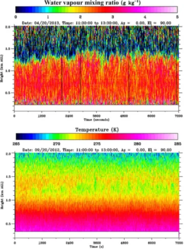
Figure 5. Time–height cross section of water vapour mixing ra-tio(a)and temperature(b)in the same time interval considered in Fig. 4.
13:30 UTC. This is the time interval that we selected for the turbulence analysis.
In order to achieve a sufficiently high signal-to-noise ra-tio (SNR) and, consequently, an acceptably low noise error level, a running average over 3 points was considered for the water vapour mixing ratio data, which translates into a re-duced vertical resolution of 90 m. No average was applied to the temperature data, keeping the original vertical resolution of 30 m.
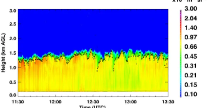
Figure 4 illustrates the time–height plot of the particle backscatter coefficient at 1064 nm,βpar, between 11:30 and
13:30 UTC on 20 April 2014. The figure reveals the presence of a significant aerosol loading within the boundary layer (with values of βparin the range 0.3–1.4×10⁻⁶m−1sr−1),
tracing the presence of a well-mixed and quasi-stationary CBL at this time of the day, extending up to a height of approximately 1300 m. The figure also reveals the presence of alternating updraughts and downdraughts.βparwas
deter-mined based on the application of a Klett-modified approach (Di Girolamo et al., 1995, 1999). The identification of the CBL height and the monitoring of its variability is made pos-sible by exploiting aerosols to act as atmospheric tracers.
The mean CBL height,zi, is an important scaling variable for turbulence profiles. The evolution of the instantaneous CBL heightz′i (black dots in Fig. 4) was determined through the application of a conventional approach based on the de-tection of the strongest gradient in the aerosol backscatter signal (see, among others, Pal et al., 2010; Haeffelin et al., 2012; Milroy et al., 2012; Summa et al., 2013). Within the considered time interval,z′i is found to be characterised by a limited variability, with a mean value zi of 1290 m a.g.l, and a standard deviation of 75 m. The minimum and max-imum values ofz′i during the observation period are 1140 and 1440 m a.g.l., respectively. This result is in very good agreement with the simultaneous measurements performed by the University of Hohenheim Differential Absorption Li-dar (UHOH-DIAL; Wagner et al., 2013; Späth et al., 2016), deployed in Hambach, approx. 4 km E–SE, with a mean value of 1295 m and a standard deviation of 86 m (Muppa et al., 2016).zi is used in the remaining part of the paper to de-termine the normalised height scalez/zi. Particle backscatter coefficient data can also be used to identify the presence of aerosol layers and/or clouds within and above the CBL, with an effective demonstrated capability to detect cloud bases and tops (the latter in the case of cloud optical thickness typ-ically smaller than 2, Di Girolamo et al., 2009b).
Figure 5 illustrates the time–height cross section of water vapour mixing ratio (Fig. 5a) and temperature (Fig. 5b) for the same time interval considered in Fig. 4. Figure 5a and b clearly highlights the large variability of water vapour mix-ing ratio and temperature within the CBL associated with the presence of alternating updraughts and downdraughts. The largest variability of both water vapour mixing ratio and temperature is observed in the interfacial layer, as a result of the penetration of the warm humid air rising from the ground and the entrainment of cool dry air from the free troposphere. Figure 5b also reveals the presence of decreas-ing temperatures within the CBL up to a minimum around 1200–1300 m and an appreciable temperature inversion (ap-prox. 1 K) above.
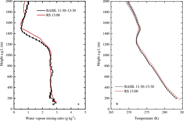
Figure 6 illustrates the mean profile for water vapour mix-ing ratio (Fig. 6a) and temperature (Fig. 6b) as measured by BASIL over the same time interval considered in Fig. 4 (11:30–13:30 UTC on 20 April 2013), together with the cor-responding profiles measured by the radiosonde launched at 13:00 UTC from the nearby site of Hambach. The water vapour mixing ratio profiles from BASIL and the radiosonde are found to agree within 0.2 g kg−1 in the mixed layer. A
larger deviation is found in the interfacial layer (0.5 g kg−1).
0 200 400 600 800 1000 1200 1400 1600 1800 2000
0 1 2 3 4 5
BASIL 11:30– 13:30 RS 13:00
Water vapour mixing ratio (g kg )
Hei
g
h
t a
.g.
l.
(
m
)
0 200 400 600 800 1000 1200 1400 1600 1800 2000
265 270 275 280 285
BASIL 11:30– 13:30 RS 13:00
Temperature (K)
H
eig
h
t a
.g
.l.
(
m
)
a b
–1
Figure 6. Mean water vapour mixing ratio(a)and temperature(b) profiles measured by BASIL on 20 April 2013 between 11:30 and 13:30 UTC, together with the corresponding profiles as measured by a radiosonde launched at 13:00 UTC from the nearby site of Hambach. Noise error bars are also shown.
the wind and the consequent deviation of its atmospheric path from the vertical. In the presence of intense convective activ-ity, deviations from the sounding data are also possible for radiosondes launched from the lidar site. In this case humid air updraughts and dry air downdraught may have lengths of a few kilometres; consequently the radiosonde can capture different features during its ascent within the CBL with re-spect to the lidar. This property makes lidar systems much more suitable for studying turbulence statistics than in situ sounding systems. In fact, because of the capability of the former to monitor the vertical air column above the station as opposed to radiosondes undergoing a horizontal drift during their ascent and, consequently, a deviation from the vertical, lidar systems guarantee the capability to measure turbulence statistics within the turbulent eddies involved in the bound-ary layer mixing processes. Similar considerations apply to the comparison between BASIL and the radiosonde in terms of temperature profile (Fig. 6b). In this case, the deviation be-tween the two sensors is∼=0.5 K throughout the CBL, with BASIL being characterised by systematically smaller values than the radiosonde, while a better agreement (deviation not exceeding 0.3 K) is observed in the free troposphere above the CBL top. In this respect, it is to be noticed that the se-quence of consecutive radiosondes launched during IOP 5 (at 09:00, 11:00, 13:00 UTC, not shown here) reveals the oc-currence of vertical profiles characterised by an almost con-stant potential temperature values within the mixed layer, as
expected for a well-mixed CBL, with potential temperature constant value progressively increasing with time. Consider-ing that Raman lidar data in Fig. 6 are averaged over a 2 h period (11:30–13:30 UTC) which is largely anticipating the radiosonde launch time (at 13:00 UTC), the systematically smaller temperature values of BASIL with respect to the ra-diosonde within the CBL are easily justifiable.
4 Turbulence analysis methodology and results 4.1 Methodology
In CBL turbulence studies, the instantaneous value of a mea-sured atmospheric variable,x(z, t ), at heightz, can be ex-pressed as the sum of three terms: a slowly varying or even constant term,x (z), where the overbar represents the time average over the considered temporal interval for the turbu-lence analysis, a fluctuation or perturbation term,x′(z, t )and
a system noise term,ε(z, t ), following the equation:
x (z, t )=x (z)+x′(z, t )+ε (z, t ) . (11)
x (z)can be derived by applying a linear fit to the data over the time period when the turbulent processes are studied (typ-ically 60–120 min, 120 min in our case).
a CBL in a quasi-stationary state, a linear fit is applied to the atmospheric variable time series.
For any measured atmospheric variable, as atmospheric variance and the noise variance are uncorrelated, total vari-ance can be expressed as follows (Lenschow et al., 2000):
(xm′(z))2=(xa′(z))2+(xn′(z))2, (12)
with(xm′(z))2 being the total measured variance,(xa′(z))2
being the atmospheric variance and(xn′(z))2being the noise
variance.
Different procedures may be considered to separate atmo-spheric variance from noise variance in the total measured variance. The autocovariance method is probably the most effective and straightforward among these procedures. This method is based on the consideration that atmospheric tuations are correlated in time, while instrumental noise fluc-tuations are uncorrelated (Lenschow et al., 2000). This ap-proach allows us to determine atmospheric variance based on the computation of the autocovariance function (ACF) for the considered atmospheric variable and then extrapolating this function to zero lag based on the application of a power-law fit. As specified in Lenschow et al. (2000), the autoco-variance function at zero lag represents the total measured variance and, consequently, the noise variance can be deter-mined as the difference between the autocovariance function extrapolated to zero lag and its value at zero leg.
An alternative approach is represented by the spectral method. In this case, the power spectrum of the atmospheric variable fluctuations is computed and the constant white noise level close to the Nyquist frequency is evaluated. Both the spectral method, based on the assumption that the sys-tem noise is white, and the autocovariance method allow us to verify whether the major part of the turbulent fluctuations is resolved through the measurements, either by comparing the high-frequency component of the spectrum with the the-oretical decay in the inertial subrange or by fitting the turbu-lent structure function to the autocovariance function. Thus, there is no reason to transfer the data in the spectral domain for these applications and, because of that, the data analy-sis was kept in the time domain. Furthermore, while both approaches were considered and tested on the water vapour and temperature data in this paper, the autocovariance tech-nique (see Fig. 1) is to be preferred because of its capability to directly determine system noise variance by means of the Fourier transformation of the autocovariance function, with-out introducing additional uncertainties (Wulfmeyer et al., 2010).
Preliminary preprocessing steps have to be applied to the data before both techniques can be applied. In general, before any further processing, spikes must be detected and flagged, as they negatively affect the calculation of turbulent variables (Senff et al., 1996). In fact, the presence of spikes in the time series may have a significant impact on the computations of higher-order moments of the turbulent statistics. Spikes in
water vapour and temperature profiles primarily result from non-linear effects associated with the application of retrieval algorithms, these being likely to happen especially at low to-noise levels (Di Girolamo et al., 2008). Low signal-to-noise levels are typically found in the daytime Raman li-dar water vapour and temperature measurements at heights above 3–5 km. This height varies depending on the consid-ered variable (being lower for water vapour and higher for temperature) or in the presence of clouds as a result of the laser beam attenuation. For the application considered in this paper, i.e. the characterisation of turbulent processes within the CBL, the vertical range of interest is up to 2000 m, and within this range the signal-to-noise level of rotational and vibrational Raman signals is typically large enough to refrain from applying the spike removal algorithm to the data. Addi-tionally, for the specific case study considered in this paper, clouds are completely missing within the CBL; consequently the application of the spike removal algorithm to the lidar data returns a data set with almost no data removed. How-ever, there may be missing data or data gaps generated in the adaptation of the temporal resolution; because of this, a spike detection algorithm (McNicholas and Turner, 2014) is routinely applied to the data before either the autocovariance method or the spectral method are applied.
4.2 Turbulent fluctuations and corresponding autocovariance functions
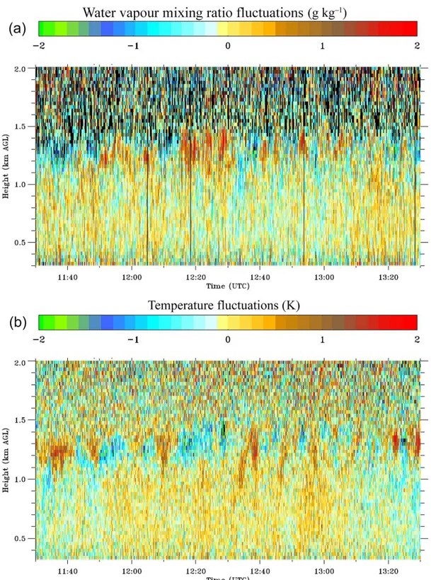
Figure 7 illustrates the time–height cross section of water vapour mixing ratio (Fig. 7a) and temperature fluctuations (Fig. 7b) in the same time interval considered in Fig. 4. Pos-itive and negative humidity and temperature fluctuations are present within the CBL. In the interfacial layer, the fluctua-tions become larger than they were below. More specifically, instantaneous water vapour fluctuations are within±0.5 in the mixed layer and±1 g kg−1in the interfacial layer, while instantaneous temperature fluctuations are within±0.5 K in the mixed layer and±1 K in the interfacial layer. In the free troposphere humidity and temperature fluctuations are al-most completely missing and the observed variability is pri-marily driven by instrumental noise.
Figure 7.Time–height cross section of water vapour mixing ratio(a)and temperature fluctuations(b)in the same time interval considered in Fig. 4.
and 1410 m indicate a larger atmospheric variance at these heights, as a result of the large atmospheric variability within the interfacial layer.
4.3 Measurements of higher-order moments
-200 -100 0 100 200 0,0 0,1 0,2 0,3 0,4 0,5 0,6 0,7 A u to co v ar ia n ce f u n ct io n ( g k g ) 2 -2 Lag (s) 420 m 630 m 810 m 1020 m 1230 m 1410 m 1620 m S tr. funct. 1230 m S tr. funct. 1410 m
-200 -100 0 100 200
0,0 0,1 0,2 0,3 0,4 0,5 0,6 A u to co v ar ia n ce fu n ctio n (K 2 ) Lag (s) 420 m 630 m 810 m 1020 m 1230 m 1410 m 1620 m S tr. funct. 1230 m S tr. funct. 1410 m (a)
(b)
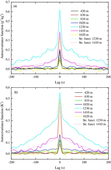
Figure 8. Autocovariance functions obtained from the measured water vapour mixing ratio(a)and temperature(b)fluctuations in the same time interval considered in Fig. 4. Autocovariance functions are displayed for the height levels between 400 and 1600 m a.g.l., i.e. 0.3 to 1.25zi, for lags from−200 to 200 s.
The integral scale can be considered an estimate of the mean size of the turbulent eddies involved in the boundary layer mixing processes. The integral scale of both water vapour mixing ratio and temperature fluctuations is found to have large values (also in excess of 200, up to 500 s for water vapour) in the lower portion of the CBL up to∼=750 m (i.e.
z/zi< 0.6). Values of the integral scale for water vapour mix-ing ratio fluctuations in the upper portion of the CBL (above 750 m) are in the range 70–125 s, with a peak value of 125 s at 1230 m (i.e.z/zi =0.95). These values are in agreement with those reported for water vapour by Wulfmeyer et al. (2010, 70–130 s) and by Turner et al. (2014a, 120–140), as well as with the simultaneous nearby measurements performed by the UHOH-DIAL, with values in the range 60–130 s (Muppa et al., 2016). Values of the integral scale for temperature fluc-tuations in the upper portion of the CBL are in the range 75–225 s, with a peak value of 225 s around the top of the
CBL (at 1310 m). These values are in agreement with those reported by Behrendt et al. (2015, 40–120 s) in a different case study, for the nearby site of Hambach. Values of the in-tegral scale throughout the CBL for both water vapour and temperature fluctuations are much larger than the temporal resolution used for the measurements (10 s), which demon-strates that the considered temporal resolution is high enough to characterise the major part of turbulence inertial subrange and, consequently, resolve the major part of the CBL turbu-lent fluctuations.
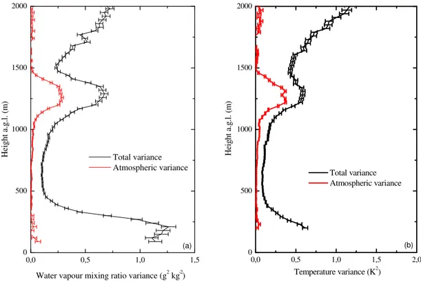
Figure 10 shows the vertical profiles of atmospheric and total variance for water vapour mixing ratio (panel a) and temperature (panel b), including noise errors. Water vapour mixing ratio variance is almost zero up to ∼=750 m (i.e.
z/zi=0.6). It remains small (< 0.05 g2kg−2) in the mid-dle and upper portion of the CBL (750 m <z< 1100 m, i.e. 0.6 <z/zi< 0.85), and it significantly increases in the inter-facial layer due to the entrainment effects. The maximum of the variance profile in the interfacial layer is 0.287 g2kg−2 at 1260 m (i.e.z/zi=0.98), with 0.051 and 0.034 g2kg−2 being the sampling error and noise error, respectively. The near-zero values in the lower portion of the CBL are typical and indicate weak forcing from the surface. In the interfa-cial layer, the variance reaches a maximum as a result of the large water vapour mixing ratio variability which is gener-ated by the vertical exchange associgener-ated with the strong up-draughts and downup-draughts (Wulfmeyer et al., 2010; Turner et al., 2014a; Muppa et al., 2016). Variance values at the top of the CBL are in good agreement with those reported by Wulfmeyer (1999a, b, 0.1–0.2 g2kg−2), Lenschow et
al. (2000, 0.1–0.2 g2kg−2) and Kiemle et al. (1997, 0.3–
0.45 g2kg−2), as well as with the simultaneous nearby
mea-surements by the UHOH-DIAL, with a peak value in the in-terfacial layer of 0.39 g2m−6, corresponding to 0.19 g2kg−2. The full width at half maximum of peak variance in the en-trainment zone is 240 m, i.e. 0.19z/zi, in agreement with measurements reported by Wulfmeyer et al. (2010, 0.16z/zi) and by Turner et al. (2014a, 0.15 z/zi). Values of water vapour mixing ratio variance decrease above the CBL top to approach zero around 1500 m.
The temperature variance remains smaller than 0.1 K2 in the middle and upper portion of the CBL up to 1150 (i.e. z/zi< 0.9). Larger values are observed in the inter-facial layer, with a maximum of 0.260 K2 at 1310 m (i.e.
0 500 1000 1500 2000
0 200 400 600 800
Water vapour mixing ratio integral scale (s)
He
ig
ht
a
.g.
l.
(m
)
0 500 1000 1500 2000
0 200 400 600 800
Temperature integral scale (s)
He
ig
h
t a
.g.l
. (m)
(a) (b)
Figure 9.Integral scale of water vapour mixing ratio(a)and temperature fluctuations(b)computed for the same time interval considered in Fig. 4.
0 500 1000 1500 2000
0,0 0,5 1,0 1,5
Total variance A tmospheric variance
Water vapour mixing ratio variance (g kg )2 - 2
H
ei
g
ht
a.g.l. (m
)
0 500 1000 1500 2000
0,0 0,5 1,0 1,5 2,0
Total variance A tmospheric variance
Temperature variance (K2)
H
eig
h
t a
.g
.l.
(
m
)
(a) (b)
Figure 10.Vertical profiles of atmospheric and total variance for water vapour mixing ratio(a)and temperature(b)computed for the same time interval considered in Fig. 4. In the figure the error bars represent only the noise error.
et al. (2016). It is to be noticed that both water vapour mix-ing ratio and temperature variance are characterised by very small sampling and noise errors, which makes the quality of
0 500 1000 1500 2000
-0,05 0,00 0,05 0,10 0,15 0,20
Third-order moment (g kg )3 -3
Hei
g
ht
a.g.l
. (m
)
0 500 1000 1500 2000
-0,10 -0,05 0,00 0,05 0,10 0,15 W ater vapour mixing ratio
Temperature
Third-order moment (K )3
H
ei
g
h
t (
m
)
(a) (b)
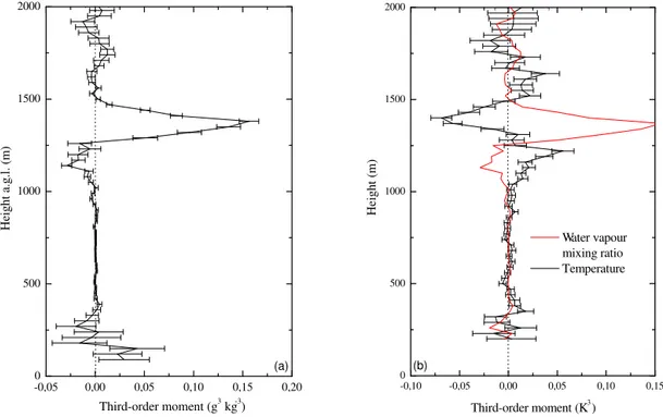
Figure 11.Vertical profiles of the third-order moment for water vapour mixing ratio(a)and temperature(b)computed for the same time interval considered in Fig. 4. In the figure the error bars represent only the noise error.
Figure 11 illustrates the vertical profiles of the third-order moment for water vapour mixing ratio (panel a) and temper-ature (panel b). The third-order moment of a variable quanti-fies the degree of asymmetry of its distribution, with positive values indicating a right-skewed distribution (with the mode smaller than the mean) and negative values indicating a left-skewed distribution (with the mode larger than the mean). Again, third-order moment estimates are characterised by very small errors, which testify the high quality of the present measurements of this turbulent variable. In Fig. 11 values of the third-order moment of water vapour mixing ratio fluctu-ations are found to be close to zero between 400 and 900 m (i.e. for 0.3zi<z< 0.7zi)and are negative between 900 and 1290 m (i.e. for 0.7 zi<z<zi), with a negative peak value of−0.029±0.005 g3kg−3at 1140 m. A large positive peak is observed just above the CBL top, with a maximum of 0.156±0.009 g3kg−3at 1380 m (z=1.07zi).
Negative values for the water vapour mixing ratio third-order moment in the upper portion of the CBL is the result of the sharp entrainment of dry air pockets into the bound-ary layer, which gradually mix with the environmental air (Couvreux et al., 2005, 2007; Wulfmeyer et al., 2010, 2016; Turner et al., 2014a). Positive values for the water vapour mixing ratio third-order moment above the top of the CBL are associated with narrow, but strong, convective plumes that penetrate up to this height. The sign and shape of the third-order moment at the top of the boundary layer may also depend on the humidity gradient above the CBL (Cou-vreux et al., 2007). The near-zero third-order moment values
in the mixed layer (z/zi< 0.7) are attributable to a symmet-ric transport process of moisture (Mahrt, 1991; Wulfmeyer et al., 2010).
The temperature third-order moment shows values close to zero (< 0.01 K3)up to 1100 m (z/zi< 0.85) and slightly pos-itive values between 1100 and 1310 m (0.85zi<z< 1.02zi), with a positive peak of 0.055 K3at 1220 m. Above 1250 m it becomes negative, with a negative peak of−0.067±0.01 K3
vari-0 500 1000 1500 2000
-0,05 0,00 0,05 0,10 0,15 0,20 0,25 0,30
Fourth-order moment (g kg )4 -4
H
eigh
t a.g.l. (m
)
0 200 400 600 800 1000 1200 1400 1600 1800 2000
-0,2 -0,1 0,0 0,1 0,2 0,3 0,4 0,5 0,6 0,7 0,8 0,9 1,0
Fourth-order moment (K )4
Heigh
t (m)
(a) (b)
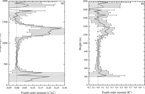
Figure 12.Vertical profiles of the fourth-order moment for water vapour mixing ratio(a)and temperature(b)computed for the same time interval considered in Fig. 4. In the figure the error bars represent only the noise error.
able gives an indication of the steepness of its distribu-tion and the width of its peak. Water vapour mixing ra-tio fourth-order moment is almost zero up to ∼=750 m (i.e.
z/zi=0.6), remains smaller than 0.02 g4kg−4 in the mid-dle and upper portion of the CBL (750 m <z< 1100 m, i.e. 0.6 <z/zi< 0.85) and increases above 1100 m, reaching its maximum of 0.28±0.13 g4kg−4around the top of the CBL (at 1350 m). It gets again close to zero above 1530 m. Similarly, temperature fourth-order moment is almost zero (< 0.05 K4)up to 1100 m (i.e.z/zi=0.85) and has positive values above, reaching a positive peak of 0.24±0.10 K4)
around the top of the CBL (at 1370 m, i.e. z/zi=1.06). Again, it becomes smaller than 0.05 K4 above 1500 m (i.e.
z/zi=1.15).
Besides the third- and fourth-order moments, atmospheric skewness and kurtosis have been determined for both water vapour mixing ratio and temperature fluctuations. Figure 13 illustrates the vertical profiles of skewness (panel a) and kur-tosis (panel b) for water vapour mixing ratio and tempera-ture. Values of water vapour mixing ratio skewness are in very good agreement with those reported by Wulfmeyer et al., 2010, with positive values (up to 1.5) in the lower portion of the CBL (up to 800 m, i.e.z/zi=0.65) and negative val-ues (down to−1) in the middle and upper portion of the CBL (800 <z< 1290 m, i.e. 0.65 <z/zi< 1.00). Large positive val-ues are found within the entrainment zone and just above the CBL top (with a maximum of approx. 5 at 1400 m, i.e.
z/zi=1.15), which testifies the presence of humidity fluctu-ations strongly deviating from a normal distribution. Values
and vertical structure of water vapour mixing ratio skewness are also in good agreement with the simultaneous and nearby measurements performed by the UHOH-DIAL (Muppa et al., 2016), with negative values (down to−1.16) in the middle and upper portion of the CBL (0.35 <z/zi< 1.00) and posi-tive values just above the PBL top (with a maximum of ap-prox. 1 atz/zi =1.05). They also agree with the measure-ments reported by Turner et al. (2014a), with negative values (down to∼ −1) up to the CBL top, zero values aroundzi and positive values just above the CBL top (with a maximum of approx. 1 atz/zi=1.1).
Temperature skewness has a negative peak (∼ −4) at 500 m, i.e.z/zi=0.4, positive peaks (∼8 and 4) at 890 and 1100 m (i.e. z/zi=0.7 and z/zi=0.85) and negative val-ues within the entrainment zone and just above the CBL top (with a peak value of∼ −7 at 1460 m, i.e.z/zi=1.13), in good agreement with measurements reported by Behrendt et al. (2015, 40–120 s) for the nearby site of Hambach in a dif-ferent case study. Again, values of skewness within the en-trainment zone and just above the CBL top are found to be large, as expected for temperature fluctuations strongly devi-ating from a normal distribution.