Comparisons of polar processing diagnostics from 34 years of the ERA-Interim and MERRA reanalyses

(1)

ACPD

14, 31361–31408, 2014

Comparisons of polar processing diagnostics

Z. D. Lawrence et al.

Title Page

Abstract Introduction

Conclusions References

Tables Figures

◭ ◮

Back Close

Full Screen / Esc

Printer-friendly Version Interactive Discussion

Discussion

P

a

per

|

Discussion

P

a

per

|

Discussion

P

a

per

|

Discussion

P

a

per

|

Atmos. Chem. Phys. Discuss., 14, 31361–31408, 2014 www.atmos-chem-phys-discuss.net/14/31361/2014/ doi:10.5194/acpd-14-31361-2014

This discussion paper is/has been under review for the journal Atmospheric Chemistry and Physics (ACP). Please refer to the corresponding final paper in ACP if available.

Comparisons of polar processing

diagnostics from 34 years of the

ERA-Interim and MERRA reanalyses

Z. D. Lawrence1, G. L. Manney1,2, K. Minschwaner1, M. L. Santee3, and A. Lambert3

1

New Mexico Institute of Mining and Technology, Socorro, NM, USA 2

NorthWest Research Associates, Socorro, NM, USA 3

Jet Propulsion Laboratory, California Institute of Technology, Pasadena, CA, USA

Received: 24 October 2014 – Accepted: 6 November 2014 – Published: 12 December 2014

Correspondence to: Z. D. Lawrence (zlawrenc@nmt.edu)

(2)

ACPD

14, 31361–31408, 2014

Title Page

Tables Figures

◭ ◮

Back Close

Full Screen / Esc

Discussion

P

a

per

|

Discussion

P

a

per

|

Discussion

P

a

per

|

Discussion

P

a

per

|

Abstract

We present a comprehensive comparison of polar processing diagnostics derived from the National Aeronautics and Space Administration (NASA) Modern Era Retrospective-analysis for Research and Applications (MERRA) and the European Centre for Medium-Range Weather Forecasts (ECMWF) Interim Reanalysis (ERA-Interim). We 5

use diagnostics that focus on meteorological conditions related to stratospheric chem-ical ozone loss based on temperatures, polar vortex dynamics, and air parcel trajec-tories to evaluate the e_ﬀects these reanalyses might have on polar processing stud-ies. Our results show that the agreement between MERRA and ERA-Interim changes significantly over the 34 years from 1979 through 2013 in both hemispheres, and in 10

many cases improves. By comparing our diagnostics during five time periods when an increasing number of higher quality observations were brought into these reanal-yses, we show how changes in the data assimilation systems (DAS) of MERRA and ERA-Interim a_ﬀected their meteorological data. Many of our stratospheric temperature diagnostics show a convergence toward significantly better agreement, in both hemi-15

spheres, after 2001 when Aqua and GOES (Geostationary Operational Environmental Satellite) radiances were introduced into the DAS. Other diagnostics, such as the win-ter mean volume of air with temperatures below polar stratospheric cloud formation thresholds (VPSC) and some diagnostics of polar vortex size and strength, do not show

improved agreement between the two reanalyses in recent years when data inputs 20

into the DAS were more comprehensive. The polar processing diagnostics calculated from MERRA and ERA-Interim agree much better than those calculated from earlier reanalysis datasets. We still, however, see fairly large relative biases in many of the di-agnostics in years prior to 2002, raising the possibility that the choice of one reanalysis over another could significantly influence the results of polar processing studies. Af-25

(3)

ACPD

14, 31361–31408, 2014

Title Page

Tables Figures

◭ ◮

Back Close

Full Screen / Esc

Discussion

P

a

per

|

Discussion

P

a

per

|

Discussion

P

a

per

|

Discussion

P

a

per

|

1 Introduction

The depletion of stratospheric ozone in the polar regions is a consequence of chemical processing that is strongly dependent upon meteorological conditions (e.g., Solomon, 1999). This polar processing takes place within the stratospheric vortices that form over the Earth’s poles in the fall and persist into spring. These polar vortices act as 5

strong barriers to transport and mixing of air across their edges (e.g., Schoeberl et al., 1992; Manney et al., 1994a), providing a pool of isolated air inside them where po-lar processing can take place (e.g., Schoeberl et al., 1992). The lower stratospheric processes that lead to chemical ozone destruction include the development of polar stratospheric clouds (PSCs), denitrification via sedimentation of PSCs, and conversion 10

of inert chlorine reservoirs to ozone-destroying forms by reactions on the surfaces of PSCs (e.g., Solomon, 1999). Because these phenomena depend critically on temper-atures and winds throughout the lower stratosphere, diagnostics related to ozone loss (e.g., WMO, 2007, 2011; Manney et al., 2011, and references therein) require fields (e.g., winds) and data coverage (e.g., vertically-resolved, hemispheric, multiannual) 15

that cannot be obtained from individual measurement systems such as satellites and radiosonde networks. As a result, the global analyses of meteorological fields provided by data assimilation systems (DAS) that combine many of these measurements are invaluable for polar processing and ozone loss studies. Numerous such DAS analy-ses are now available, facilitating both observational and modeling studies of polar 20

processing. However, variations in the representation of meteorological conditions are expected because of differences in the model formulations and resolution, assimilation methods, and assimilated products. The existence of these di_fferences raises the pos-sibility of conflicting results and conclusions between similar studies conducted using different DAS analyses.

25

(4)

ACPD

14, 31361–31408, 2014

Title Page

Tables Figures

◭ ◮

Back Close

Full Screen / Esc

Discussion

P

a

per

|

Discussion

P

a

per

|

Discussion

P

a

per

|

Discussion

P

a

per

|

especially PSC formation and chlorine activation, are commonly used. Some of these diagnostics, such as the volume of air below PSC temperature thresholds (V_PSC), have been found to have strong links to total column ozone depletion (e.g., Rex et al., 2004; Tilmes et al., 2006; Harris et al., 2010). While some studies have linked changes in V_PSCto an expectation of colder winters and greater ozone loss in the Arctic with global 5

climate change (Rex et al., 2004, 2006), others do not support this conclusion (Hitch-cock et al., 2009; Pommereau et al., 2013; Rieder and Polvani, 2013). Climate model projections of future ozone loss are also highly uncertain (Charlton-Perez et al., 2010). Thus, the prediction of future ozone loss is still problematic, and improvements in such predictions will require better understanding of the uncertainties and potential biases in 10

representation of the meteorological conditions upon which polar processing depends so critically in commonly-used DAS.

Previous studies have recognized the importance of understanding the sensitivity of polar processing and ozone loss quantification to di_ﬀerent datasets: Davies et al. (2002) showed that two SLIMCAT chemical transport model (CTM) runs driven by hori-15

zontal winds and temperatures from the ECMWF (European Centre for Medium-Range Weather Forecasts) and Met O_ffice DAS led to significantly di_fferent patterns of deni-trification and chlorine activation, and consequently large di_fferences in ozone loss of nearly 20 %. Similarly, Santee et al. (2002) found significant discrepancies in PSC for-mation and composition between model runs that used Met O_ffice temperatures with 20

and without a 3 K reduction. Sinnhuber et al. (2011) found that reducing the temper-atures from the ECMWF operational analyses by 1 K in CTM runs for the 2010/2011 Arctic winter resulted in a substantial increase in ozone loss. Brakebusch et al. (2013) reduced GEOS-5 (Goddard Earth Observing System model, version 5) temperatures by 1.5 K in a Whole Atmosphere Community Climate Model simulation of ozone for 25

(5)

Man-ACPD

14, 31361–31408, 2014

Title Page

Tables Figures

◭ ◮

Back Close

Full Screen / Esc

Discussion

P

a

per

|

Discussion

P

a

per

|

Discussion

P

a

per

|

Discussion

P

a

per

|

ney et al. (2005b) and Feng et al. (2005) discuss many issues with polar temperatures from the ECMWF 40 year reanalysis (ERA-40), including periods with large spurious vertical oscillations in polar winter temperature profiles (e.g., Simmons et al., 2005). In intercomparisons of temperature diagnostics related to Arctic polar processing of several meteorological analyses, Manney et al. (2003) found that the area with tem-5

peratures below PSC thresholds varied by up to 50 % between diﬀerent analyses, and potential PSC lifetimes diﬀered by several days. Manney et al. (2005a) argued that several reanalyses (the datasets referred to therein as the National Centers for Envi-ronmental Prediction and National Center for Atmospheric Research (NCEP-NCAR) reanalysis, NCEP–DOE reanalysis-2, and ERA-40) were unsuitable for stratospheric 10

and polar processing studies.

Since the above-mentioned studies, significant advances have been made in mod-eling and data assimilation, and several additional datasets have become available for constraining the DAS. Long-term reanalysis systems have become much more widely used, and the long-term records of global meteorology based on observa-15

tional data that they provide are increasingly critical for climate studies. The grow-ing use of reanalysis datasets demands intercomparisons that quantify the di_ﬀ er-ences between them. While numerous intercomparisons have been done (see, e.g., https://reanalyses.org/atmosphere/inter-reanalysis-studies-0), most focus primarily on tropospheric and/or near-surface processes. A few studies have also compared tropi-20

cal upper tropospheric processes in commonly used reanalyses (e.g., Schoeberl and Dessler, 2011; Fueglistaler et al., 2013). Rieder and Polvani (2013) showed calcula-tions of one polar processing diagnostic, VPSC, from three reanalyses. However, no

comprehensive intercomparisons of diagnostics pertinent to polar processing in the winter lower stratosphere have been done for the reanalyses that are currently in 25

(6)

ACPD

14, 31361–31408, 2014

Title Page

Tables Figures

◭ ◮

Back Close

Full Screen / Esc

Discussion

P

a

per

|

Discussion

P

a

per

|

Discussion

P

a

per

|

Discussion

P

a

per

|

study because of their extensive application in numerous stratospheric studies. Rather than focusing on specific seasons and/or a single hemisphere, we present most of our diagnostics for the 1979–2013 record of the reanalyses for both Arctic and Antarctic winters. We examine the potential correlation of biases between the analyses over the above time period with the timing of changes in observations ingested by their DAS. It 5

is diﬃcult to directly assess the accuracy of reanalyses because there are few, if any, independent measurements (i.e., not used in the assimilation) of temperature available that span the full periods of those analyses; the degree of agreement between re-analyses is thus an important indicator of their inherent uncertainties and the potential impact of those uncertainties on polar processing studies.

10

In Sect. 2 we describe the datasets, relevant aspects of the assimilated observations, and the diagnostics and comparison methods we use. The results, presented in Sect. 3, comprise comparisons of polar processing diagnostics based on temperatures, polar vortex dynamics, and trajectory-based temperature histories. Our conclusions are then summarized and discussed in Sect. 4.

15

2 Data and analysis

2.1 NASA Modern Era Retrospective analysis for research and applications

MERRA is a global atmospheric reanalysis that uses version 5.2 of the Goddard Earth Observing System (GEOS) model and assimilation system. It utilizes a combination of 3D-Var assimilation and Incremental Analysis Update (IAU) (Bloom et al., 1996) to 20

apply corrections from analysis to the forecast model. The MERRA system operates natively on a 0.5◦×0.667◦ latitude/longitude grid (361×540 gridpoints) and uses a hy-brid sigma-pressure scheme with 72 vertical levels; the vertical resolution in the lower stratosphere is near 1 km. Further details about the MERRA system are given by Rie-necker et al. (2011). The MERRA data files available from NASA’s Global Modeling and 25

(7)

ACPD

14, 31361–31408, 2014

Title Page

Tables Figures

◭ ◮

Back Close

Full Screen / Esc

Discussion

P

a

per

|

Discussion

P

a

per

|

Discussion

P

a

per

|

Discussion

P

a

per

|

otherwise, the MERRA temperature data used here are from instantaneous daily files at 12:00 UT on the model levels and grid. However, the potential vorticity (PV) data from MERRA are available only on a reduced 1◦×1.25◦ latitude/longitude grid (181×288 gridpoints) with 42 pressure levels; for the purposes of this study, PV is interpolated to match the model levels and grid.

5

2.2 ECMWF Interim reanalysis

ERA-Interim (hereinafter ERA-I) is another global atmospheric data assimilation sys-tem. The goal of the ERA-I project was to improve upon ECMWF’s previous reanalysis, ERA-40, in advance of their planned next-generation reanalysis. It uses 12 h cycles of 4D-Var assimilation and a T255 spectral model with 60 vertical levels; the vertical res-10

olution in the lower stratosphere is comparable to that of MERRA. The ERA-I system is described in detail by Dee et al. (2011), and the datasets provided by ECMWF from the ERA-I archive are described by Berrisford et al. (2009). In this case, ERA-I data are used on the highest resolution regular latitude/longitude grid publicly available at 0.75◦×0.75◦(241×480 gridpoints) on the 60 model vertical levels; this grid has spac-15

ing closest to that of the Gaussian grid associated with the spectral model. As with MERRA, the ERA-I temperature and PV data used in this study are instantaneous at 12:00 UT. However, in this case the PV is derived from the provided relative vorticity, temperature, and pressure fields.

2.3 Timelines of assimilated observations

20

Since satellite observations are the primary constraint on reanalysis products at strato-spheric levels, it is useful to consider how the data evolve with the introduction of new missions and instruments: Pawson (2012) noted the eﬀect of the TOVS (Tiros Opera-tional Vertical Sounder) to Advanced TOVS (ATOVS) transition in 1998 on middle and upper stratospheric global temperature anomalies from MERRA and ERA-I. At 5 hPa, 25

(8)

ACPD

14, 31361–31408, 2014

Title Page

Tables Figures

◭ ◮

Back Close

Full Screen / Esc

Discussion

P

a

per

|

Discussion

P

a

per

|

Discussion

P

a

per

|

Discussion

P

a

per

|

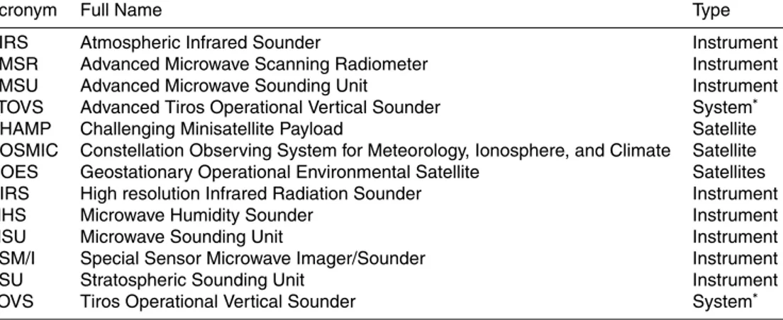
the mean annual cycle changed noticeably. Pawson asserts that these distinct dis-continuities suggest that more work is needed to properly handle SSU (Stratospheric Sounding Unit) radiances in reanalyses. Fueglistaler et al. (2013) mention that the in-troduction of COSMIC (Constellation Observing System for Meteorology, Ionosphere, and Climate) GPSRO (Global Positioning Satellite Radio Occultation) temperature data 5

in ERA-I caused a temperature shift in the tropics of about 0.5 K at 100 hPa. Simmons et al. (2014) discuss in detail the various eﬀects of the diﬀerent satellite missions and instruments on ERA-I temperature data, and perform intercomparisons with MERRA and the Japanese 55 year Reanalysis (JRA55).

In many of our diagnostics, we examine how well MERRA and ERA-I agree over the 10

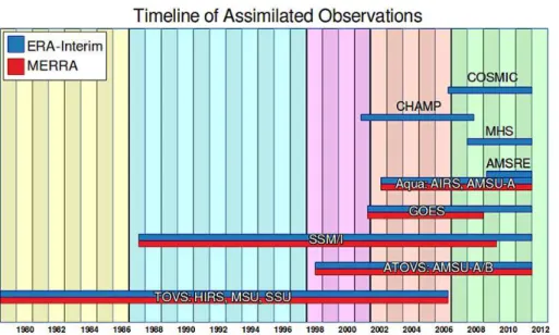
1979 to 2013 time period. The observations assimilated in the reanalyses change dra-matically over this period, and in some cases there are di_ﬀerences between MERRA and ERA-I in the timing of the changes and the observations included. Figure 1 shows a comparison of the primary satellite datasets assimilated in MERRA and ERA-I, com-piled from information in Rienecker et al. (2011), Dee et al. (2011) and Simmons et al. 15

(2014). (See Table 1 for the full names of the instruments and satellites listed in Fig. 1 and throughout this paper.) The colored regions indicate periods of years between which the data input streams change significantly; in other words, marking times when the di_ﬀerences between MERRA and ERA-I might be expected to shift. In this case, we have chosen boundaries at 1987 (when SSM/I was introduced), 1998 (when ATOVS 20

was introduced), 2002 (inclusion of CHAMP in ERA-I, and AIRS and AMSU-A in both reanalyses), and 2007 (when COSMIC was included in ERA-I).

2.4 Polar processing diagnostics and intercomparisons

Many of the diagnostics we use are described by Manney et al. (2003, 2005a, 2011), and are designed to assess a wide range of conditions related to polar processing. 25

(9)

ACPD

14, 31361–31408, 2014

Title Page

Tables Figures

◭ ◮

Back Close

Full Screen / Esc

Discussion

P

a

per

|

Discussion

P

a

per

|

Discussion

P

a

per

|

Discussion

P

a

per

|

to chemical processing and ozone destruction in the polar stratosphere. Because our focus is on assessing the eﬀects of reanalysis diﬀerences on studies of polar process-ing that takes place in the lower stratosphere, we focus in this paper on isentropic levels below about 600 K (approximately 25 km, or 30 hPa).

The importance of stratospheric temperatures to the formation of PSCs gives rise to 5

the need for temperature diagnostics. Although some recent studies have suggested that liquid PSCs play a dominant role in activating chlorine (e.g., Wegner et al., 2012; Wohltmann et al., 2013), the formation temperatures of solid nitric acid trihydrate (NAT, Hanson and Mauersberger, 1988) and ice particles remain convenient thresholds for the initiation of chlorine activation processes. In this study, we examine daily mini-10

mum temperatures, and calculations of area with temperatures below PSC thresholds (henceforth, T_min and A_PSC, respectively). We also use diagnostics derived fromT_min and A_PSC, such as the number of days during a polar winter with temperatures be-low PSC thresholds, and the volume of stratospheric air bebe-low PSC thresholds (V_PSC). ForA_PSC, vertical temperature profiles of the NAT and ice thresholds are derived us-15

ing climatological profiles of HNO₃ and H₂O mixing ratios on six per decade pressure levels (Manney et al., 2003), and interpolating to approximately co-located potential temperature surfaces (e.g., the 56.2 and 31.6 hPa levels are referenced to 490 and 580 K, respectively).V_PSCis calculated by vertically integrating eight potential tempera-ture levels between 390 and 580 K using the altitude approximation introduced by Knox 20

(1998).

Since the polar vortex provides the “containment vessel” within which polar chemical processing takes place (e.g., Schoeberl et al., 1992), we also compare diagnostics that characterize vortex strength and size. These include daily maximum PV gradients (one measure of vortex strength, e.g., Manney et al., 2011, and references therein), 25

(10)

ACPD

14, 31361–31408, 2014

Title Page

Tables Figures

◭ ◮

Back Close

Full Screen / Esc

Discussion

P

a

per

|

Discussion

P

a

per

|

Discussion

P

a

per

|

Discussion

P

a

per

|

vertically integrateAvortin the same manner asAPSCto derive the vortex fraction of low

temperature air (i.e.,V_PSC/V_vort). In all cases we use isentropic surfaces, and scale PV into “vorticity units” (s−1) (Dunkerton and Delisi, 1986; Manney et al., 1994b). MPVG is calculated as described by Manney et al. (1994a): scaled PV (sPV) is numerically di_ﬀerentiated with respect to equivalent latitude (i.e., the value of the latitude circle 5

enclosing the same area as a given PV contour); if the maximum gradient occurs at an equivalent latitude poleward of±80◦, we consider the vortex to be undefined and set the maximum gradient equal to zero. To calculate the area of the polar vortex, we use the 1.4×10−4s−1sPV contour as a simple proxy for the vortex edge (e.g., Manney et al., 2007). The total area of the vortex is then the area of the contour. The sunlit area 10

is the area inside the vortex-edge contour that is equatorward of the daily polar night latitude at 12:00 UT.

One of our diagnostics is best described as a hybrid temperature-vortex diagnostic. It is the concentricity of the polar vortex with regions of temperatures below the NAT PSC threshold (henceforth referred to as vortex-temperature concentricity, or VTC). 15

VTC is adapted from the concept of concentricity as discussed by Mann et al. (2002). We calculate it using the simple formula

VTC=1−GCDist(Vortex Centroid, Cold Region Centroid)

GCDist(Pole, Equiv. Lat. of Vortex Edge) (1)

where GCDist(x,y) is the great circle distance betweenx and y. This definition pro-vides an intuitive picture of the vortex/temperature relationships under extreme con-20

ditions: a maximum value of 1 for collocated centroids (completely concentric), and values less than or equal to 0 for a cold region centroid approximately at or outside the vortex edge. Centroid locations are calculated as described by Mitchell et al. (2011) and Seviour et al. (2013), with the 1.4×10−4s−1sPV and pressure-dependent NAT PSC temperatures as the edge values for the vortex and cold regions, respectively. For 25

(11)

ACPD

14, 31361–31408, 2014

Title Page

Tables Figures

◭ ◮

Back Close

Full Screen / Esc

Discussion

P

a

per

|

Discussion

P

a

per

|

Discussion

P

a

per

|

Discussion

P

a

per

|

were not characterized individually. Under conditions where multiple closed contours exist, VTC values may be calculated using centroids that lie completely outside of the regions of interest. While it would be important to more accurately characterize split vortices for detailed dynamical studies, this simplification does not significantly aﬀect the broad climatological comparisons we are focusing on here.

5

We also use trajectory diagnostics to examine temperature histories of air parcels; these provide important information about the potential for polar processing. Here we use a trajectory code adapted from the Lagrangian Trajectory Diagnostic (LTD) code described by Livesey (2013), which advects parcels using a fourth-order Runge–Kutta method. Our standard runs consist of 15 day forward and backward (30 days total) 10

trajectories initialized at 00:00 UT integrated with 15 min timesteps for parcels on an equal-area grid. For this paper, we initialized parcels on the 490 K potential tempera-ture surface on an equal-area grid poleward of±40◦latitude with 0.5◦×0.5◦equatorial spacing. We examine the parcels initialized in cold regions defined by T≤195 K (the approximate NAT threshold at 490 K), and the amount of time they spend below the 15

threshold before and after the initialization date. From this subset of parcels, we calcu-late and compare distributions for total time spent below 195 K (TT195) and continuous time spent below 195 K (CT195) as described by Manney et al. (2003, 2005a).

3 Results

3.1 Monthly relative biases

20

Figure 2 shows an example of the type of differences we calculate for most of the di-agnostic intercomparisons (in this caseT_min), for 1979 through 2013. The orange line showing the di_fferences for 2012/2013 provides an example of the magnitude of dif-ferences in an individual recent year. Note that there are large day-to-day variations in differences, and that the differences are largest in December 2012 and early Jan-25

(12)

ACPD

14, 31361–31408, 2014

Title Page

Tables Figures

◭ ◮

Back Close

Full Screen / Esc

Discussion

P

a

per

|

Discussion

P

a

per

|

Discussion

P

a

per

|

Discussion

P

a

per

|

SSW (Coy and Pawson, 2014). The departure of the daily average diﬀerences (thick black line) from zero suggests a persistent relative bias between the two reanalyses that dominates for much of the 34 years. Since this bias varies over the season, we define monthly relative biases between the datasets as the monthly averaged mean daily di_ﬀerences over the years in each of the periods defined in Fig. 1. These quan-5

tities provide a compact means of summarizing the agreement between the datasets for a given month and subset of years, and of comparing the magnitude of diﬀerences between comparison periods for a particular diagnostic. We refer to these as “relative” biases to emphasize that they represent biases between the two datasets, as opposed to an assessment of absolute accuracy of either. For the rest of this paper, we use the 10

convention of subtracting ERA-I from MERRA (that is, MERRA minus ERA-I) to cal-culate monthly relative biases. As such, diﬀerences in a diagnostic greater (less) than zero indicate that, on average, MERRA is greater (less) than ERA-I.

3.2 Temperature diagnostic intercomparisons

The seasonal progression of polar minimum temperatures provides an indication of 15

when conditions favor the development of PSCs. The dependence of PSC formation on a temperature threshold implies that conclusions drawn from theT_mindiagnostic are most sensitive to di_ﬀerences at the beginning and ends of the season when minimum temperatures first drop below or rise above PSC thresholds. For the Arctic, these peri-ods are typically around the beginning of December and mid-March, respectively, but 20

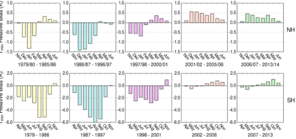
large interannual variability and the common occurrence of mid-winter SSWs can re-sult in much earlier or later threshold dates in individual years (Manney et al., 2005a, and references therein). In the Antarctic, the threshold periods tend to be in the first half of May and in mid-October. Figure 3 shows the monthly relative biases between MERRA and ERA-I at the 580 K level (∼30 hPa, corresponding to an approximateT_NAT 25

(13)

ACPD

14, 31361–31408, 2014

Title Page

Tables Figures

◭ ◮

Back Close

Full Screen / Esc

Discussion

P

a

per

|

Discussion

P

a

per

|

Discussion

P

a

per

|

Discussion

P

a

per

|

in the Arctic, which are about−1.4 K. Diﬀerences in 1998–2001, after the introduction of the ATOVS instruments, but before the introduction of the Aqua instruments, are sig-nificantly reduced over those prior to 1998. In both hemispheres, there is a distinct shift in agreement after the introduction of the Aqua instruments from 2002 onward (likely due to the vast increase in the number of observations included by assimilating AIRS 5

data). This is especially easy to see for the Antarctic, where the relative biases are reduced to values akin to those in the Arctic. In the Northern Hemisphere (NH), the shift marks the first period in which ERA-I minimum temperatures become consistently lower than those from MERRA. At lower levels down to about 460 K (not shown), the T_min relative biases are smaller in magnitude (e.g., at 490 K they are between−0.4 and 10

0.7 K in the Arctic, and−2 to 2 K in the Antarctic), and have di_ﬀerent seasonal varia-tions, with ERA-I having comparatively more months in the first three time periods with lower minimum temperatures.

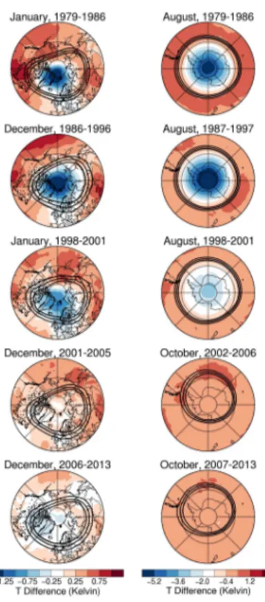
To examine the global variation of temperature di_ﬀerences between MERRA and ERA-I, Fig. 4 shows maps of mean temperature di_ﬀerences (averaged over the time 15

periods of interest from Fig. 1) for the months with the largest relative T_min biases in Fig. 3. The maps for the Arctic, with the more symmetric color bar, clearly demonstrate that the regions where MERRA is colder tend to be mostly confined between ±90◦ longitude and poleward of 60◦ latitude. This is a preferred direction for the polar vortex and cold region to be shifted o_ﬀ the pole in Arctic winters (e.g., Waugh and Randel, 20

1999). Outside of this area, ERA-I temperatures are, for the most part, lower than those from MERRA. In the Southern Hemisphere (SH), the first three time periods show that the regions that are colder in MERRA are fairly symmetric poleward of the 60◦

S latitude circle. Examination of the mean temperature fields (not shown) for these periods suggests that larger biases are associated with lower temperatures. The maps 25

(14)

ACPD

14, 31361–31408, 2014

Title Page

Tables Figures

◭ ◮

Back Close

Full Screen / Esc

Discussion

P

a

per

|

Discussion

P

a

per

|

Discussion

P

a

per

|

Discussion

P

a

per

|

show extratropical zonal-mean temperature diﬀerences between ERA-I and MERRA at 30 hPa that indicate the extratropics (±20–90◦ latitude) are colder in ERA-I than in MERRA for most of the reanalysis period. The results shown here are generally consistent with that finding, but suggest that this result does not hold true poleward of ±60◦latitude in winter/spring.

5

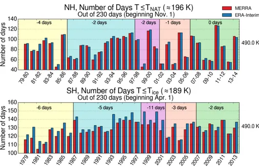
The number of days below PSC thresholds, a diagnostic derived fromT_min, for win-ters in the 1979 through 2013 period is shown at 490 K (∼56 hPa) for both hemispheres in Fig. 5; we show days belowT_ice, rather thanT_NAT, in the Antarctic because the pe-riod with temperatures below either threshold is much longer, making the diﬀerences clearer for the lower ice threshold. This diagnostic indicates the approximate duration 10

of the period with conditions conducive to polar processing. Overall, the number of cold days from ERA-I is greater than the number from MERRA in both hemispheres. The Antarctic diﬀerences before 2002 are quite large, with some years showing ERA-I hav-ing over 10 more days with temperatures below the ice PSC threshold than MERRA. At levels up to 580 K (not shown), the situation in the Antarctic is opposite; that is, there 15

are significantly more days with temperatures below the ice PSC threshold in MERRA than in ERA-I. These results, along with those discussed aboutT_min, suggest that not only may the choice of dataset have a large influence on analysis and modeling of po-lar processes in the Antarctic for years preceding 2002, but also that eﬀects may vary qualitatively and quantitatively in the vertical. In contrast to the Antarctic, the magnitude 20

of di_ﬀerences in the Arctic at higher levels up to 580 K are largely similar to those at 490 K, but with MERRA having more cold days than ERA-I.

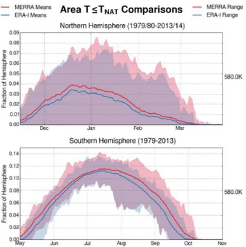
Average values for the total area with temperatures below the NAT threshold at 580 K are displayed in Fig. 6. The Arctic maximum mean area is just above 3 % of the hemi-sphere for ERA-I, while MERRA reaches nearly 4 %. In a similar fashion, the Antarctic 25

(15)

ACPD

14, 31361–31408, 2014

Title Page

Tables Figures

◭ ◮

Back Close

Full Screen / Esc

Discussion

P

a

per

|

Discussion

P

a

per

|

Discussion

P

a

per

|

Discussion

P

a

per

|

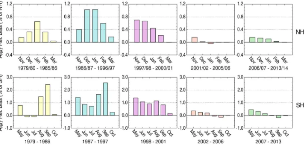
month of the season in each hemisphere are expected as these include many days that have zero biases because minimum temperatures have risen above the NAT threshold in both reanalyses. Consistent with theT_minrelative biases, there is much closer agree-ment after the first three periods. The relatively frequent occurrence of warm Arctic winters after 1998 (e.g., Manney et al., 2005a) suggests that the third Northern Hemi-5

sphere period might be less easily compared with the previous period with unusually cold Arctic winters (e.g., Pawson and Naujokat, 1999), but the marked decreases of relative biases in the SH still indicate a substantial e_ﬀect due to changes in assimilated observations. In most cases the relative biases are positive, indicating that MERRA tends to have larger cold regions than ERA-I at this level in both hemispheres. For lev-10

els below 580 K, down into the upper troposphere/lower stratosphere (UTLS) region at 390 K (not shown), MERRA still tends to have larger cold regions than ERA-I, but the conditions are diﬀerent: the relative biases are much smaller in all periods, generally lying between−1 and 1 % in the Antarctic, and−0.4 and 0.4 % in the Arctic. Although the relative biases are smaller, the same convergence towards better agreement we 15

see at 580 K is not always seen at levels below 520 K, especially in the Arctic.

3.3 Vortex diagnostic intercomparisons

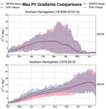
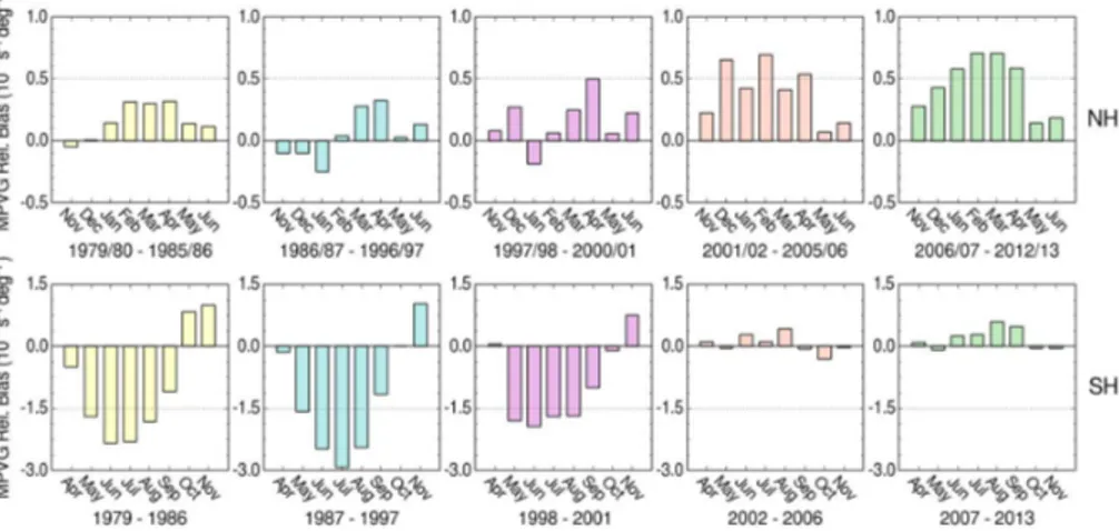
Maximum PV gradients (MPVG) indicate the strength of the polar vortex as a barrier to transport and mixing of air from lower latitudes and the cold vortex air where chlorine activation takes place (e.g., Manney et al., 2011). The seasonal evolution and mean 20

values of maximum PV gradients at 490 K are shown in Fig. 8. The primary di_ﬀerence between the hemispheres is seen in the average values; the Arctic maximum gradients tend to level oﬀat around 10−5s−1deg−1early in the season, while the Antarctic maxi-mum gradients steadily increase up to approximately 1.7×10−5s−1deg−1near the end of the season. The MPVG relative biases are shown in Fig. 9. Note that the scaling of 25

(16)

ACPD

14, 31361–31408, 2014

Title Page

Tables Figures

◭ ◮

Back Close

Full Screen / Esc

Discussion

P

a

per

|

Discussion

P

a

per

|

Discussion

P

a

per

|

Discussion

P

a

per

|

the greater MERRA MPVGs in the months when the vortex usually weakens (March or April in the Arctic, November in the Antarctic) suggest that the polar vortices as rep-resented by ERA-I tend to weaken earlier than those in MERRA. Furthermore, a shift in agreement contemporaneous with those seen in Figs. 3 and 7 is also present. In this case, however, the relative biases increase considerably for the Northern Hemi-5

sphere rather than decrease. This behavior, with agreement in the SH (NH) improving (degrading) slightly, is also seen at other vertical levels between 460 and 580 K.

Similar to A_PSC, the sunlit area of the vortex provides an approximate quantitative measure of the area on a given vertical level where chlorine-catalyzed ozone destruc-tion can take place. Diﬀerent sunlit area diagnostics have been used in detailed polar 10

processing studies to establish correlations between the coverage (e.g., Feng et al., 2007) and duration (e.g., Rex et al., 1999; Livesey et al., 2014, in preparation) of sun-light and ozone loss; these diagnostics are usually somewhat computationally inten-sive, whereas the diagnostic used here (described in Sect. 2.4 above) is simple enough to compute for multiple long-term datasets. Figure 10 shows time series averages and 15

ranges of the sunlit vortex diagnostic as a fraction of a hemisphere at 490 K. The sea-sonal variations of the sunlit vortex are very similar in both datasets. There are, how-ever, small biases that can be seen: the ERA-I Arctic polar vortex tends to be filled with slightly more sunlight than the MERRA vortex, while in the Antarctic, the bias changes over the season. Consistent with this, the sunlit vortex monthly relative biases in Fig. 11 20

show predominantly negative values in the Arctic (indicating the bias towards ERA-I), and biases that change sign in the Antarctic. Like the NH MPVG relative biases, the NH sunlit vortex relative biases increase to a maximum by the 5th time period (2007– 2013) of Fig. 1. The overall maximum relative biases occur in November and February of this final time period, both months when a substantial portion of the vortex is typi-25

(17)

ACPD

14, 31361–31408, 2014

Title Page

Tables Figures

◭ ◮

Back Close

Full Screen / Esc

Discussion

P

a

per

|

Discussion

P

a

per

|

Discussion

P

a

per

|

Discussion

P

a

per

|

especially in the Antarctic where the vortex is larger, colder, and less variable from year to year than in the Arctic. The vertical structure of the sunlit area biases (not shown) is complicated, but for recent years the ERA-I NH polar vortex tends to have a larger sunlit area than that in MERRA at levels between 460 and 550 K, while the opposite is true for the SH. The biases in sunlit vortex area shown here primarily arise from similar 5

biases in total vortex area (A_vort, not shown). However, small differences between the relative biases of sunlit and total vortex area indicate a very small effect from differing vortex positions. Examination of the relative vorticity and static stability from MERRA and ERA-I suggests a small, but persistent, global bias towards larger magnitude static stability values in ERA-I, which likely contributes to the biases in vortex size.

10

The winter mean vortex fraction of cold air diagnostic helps to identify years with con-ditions favorable for PSC formation. In the Arctic, years with low values ofV_PSC/V_vort correspond to winters with very short cold periods usually associated with a disturbed vortex and midwinter SSWs. Because of its relationship to column ozone loss, V_PSC has been used extensively in climatological ozone loss studies (e.g., Pommereau et al., 15

2013; Rex et al., 2004, 2006; Rieder and Polvani, 2013; Tilmes et al., 2006). V_vort as a stand-alone diagnostic is much less common; however, the volume of air within the vortex is an indicator of the absolute size of the region over which chemical ozone loss can occur. Figures 12 and 13 show winter mean V_PSC/V_vort for the Arctic and Antarctic, respectively, along with the corresponding winter meanV_PSC and V_vort val-20

ues separately. In general, MERRA tends to have a larger volume of cold air in both hemispheres, consistent with the largerA_NAT relative biases shown in Fig. 7. The only major exceptions are the years from 1979 to 1987 in the Antarctic, where ERA-IVice

is a bit larger than that in MERRA. The lack of improvement in agreement for V_PSC follows directly from the prior discussion ofA_NAT; since the agreement ofA_NAT between 25

(18)

ACPD

14, 31361–31408, 2014

Title Page

Tables Figures

◭ ◮

Back Close

Full Screen / Esc

Discussion

P

a

per

|

Discussion

P

a

per

|

Discussion

P

a

per

|

Discussion

P

a

per

|

Exceptions to this are in 2007–2013 in the NH, when slightly smaller MERRAV_vort val-ues emphasize the∼0.01 largerV_PSC/V_vort values seen in MERRA, and in 1979–1987 in the SH, when the∼0.02 larger ERA-I V_PSC/V_vort values represent larger cold frac-tions of smaller vortices. This analysis demonstrates several caveats for comparisons of diagnostics that rely on vertical integration, time averages, or combinations of both. 5

Their dependence on time and/or altitude can lead to cancellations and smoothing when integrated and/or time-averaged, making comparisons of the final results diﬃcult to interpret since agreement (or lack thereof) can come about for the wrong reasons. In this case, the agreement of winter meanV_PSC,V_vort, andV_PSC/V_vort between the re-analyses was a_ﬀected by the representation of several conditions. Because the relative 10

biases inA_PSCand A_vort change diﬀerently with time and altitude, better agreement at some levels does not necessarily correlate with better confidence in our knowledge of V_PSC, and consequentlyV_PSC/V_vort. This suggests that these diagnostics function better as qualitative measures, and argues for considerable caution in interpretation of their time variations or trends.

15

The concentricity of the vortex with regions of air withT ≤T_NAT (VTC) has not been widely used in polar processing studies. However, Mann et al. (2002), using a con-centricity diagnostic di_fferent from that defined here, found that di_fferent values led to dramatically di_fferent patterns of denitrification in model simulations of NAT particle growth and evaporation because differences in the position of the cold region relative 20

to the strong winds bounding the vortex can result in large di_ﬀerences in the amount of time air spends in cold regions of comparable size (Manney et al., 2003). Using ideal-ized model simulations with a constant vortex field and cold regions ranging from highly concentric to nonconcentric, Mann et al. showed that concentricity aﬀected denitrifica-tion independent of any variadenitrifica-tions in the vortex itself. Since the concentricity calculadenitrifica-tion 25

(19)

ACPD

14, 31361–31408, 2014

Title Page

Tables Figures

◭ ◮

Back Close

Full Screen / Esc

Discussion

P

a

per

|

Discussion

P

a

per

|

Discussion

P

a

per

|

Discussion

P

a

per

|

the results at the 490 K level. The total number of days shown corresponds to the num-ber of days with a valid VTC value summed over the years from the comparison time periods defined in Fig. 1 and used in the monthly relative bias plots. As evidenced by the non-overlapping colors, in most cases the ERA-I vortices spend more time at higher concentricity values (within the 0.8 to 1.0 range) in both hemispheres. Consistent with 5

the number of days below PSC thresholds shown in Fig. 5, ERA-I also tends to have more valid VTC days than MERRA in both hemispheres. The detailed implications of di_ﬀerences in concentricity are di_ﬃcult to assess, but the results of Mann et al. (2002) and Manney et al. (2003) suggest that greater concentricity in ERA-I could bias model runs driven by that reanalysis towards longer-lasting PSCs, greater denitrification, and 10

enhanced chlorine activation.

3.4 Trajectory diagnostic intercomparisons

Temperature histories along air parcel trajectories provide further information about polar processing potential beyond what can be obtained from the simple diagnostics described above. For these intercomparisons, we use isentropic trajectory calculations 15

on the 490 K surface. As discussed by Manney et al. (2003), although neglecting cross-isentropic motion would not be suitable for detailed polar processing studies, this simpli-fication allows us to e_ﬃciently run and analyze a large number of parcels for extensive intercomparisons. Following Manney et al. (2003, 2005a), we consider only the parcels that are initialized in regions with temperatures less than 195 K. With this initial filter, we 20

examine the total and continuous amounts of time that these parcels spend at temper-atures below 195 K (TT195 and CT195, respectively) before and after the initialization date, and the mean temperature of the parcels over the full run. The TT195 diagnostic captures the total exposure of an air mass to temperatures low enough for PSC forma-tion and thus acts as a proxy for cumulative chlorine activaforma-tion; CT195 better represents 25

(20)

ACPD

14, 31361–31408, 2014

Title Page

Tables Figures

◭ ◮

Back Close

Full Screen / Esc

Discussion

P

a

per

|

Discussion

P

a

per

|

Discussion

P

a

per

|

Discussion

P

a

per

|

show trajectory calculations initialized on 10 January 1996 and 24 January 2011 for the NH, and 17 September 1988, 13 September 2002, and 25 May 2011 for the SH. These dates have been chosen to span a range of conditions representative of the in-terannual variability in both hemispheres, and in some cases to compare with previous studies using the same diagnostics. Several other cases have been investigated for 5

each hemisphere; the results shown here are representative.

Figure 15 summarizes the trajectory diagnostics for the NH. Overall, the parcel his-tograms for TT195 and CT195 are very similar between MERRA and ERA-I, with con-sistent distributions, peaks, and average values. The number of parcels included in the calculations indicate that MERRA has slightly larger regions of cold air, but the aver-10

age values of the distributions only di_ffer by approximately 0.05 days (∼1.2 h) for TT195 and 0.5 days (∼12 h) for CT195. Where there are small differences, they are consistent with minor spatial differences in maps of the parcels (not shown), which are also other-wise very similar. In investigating other NH winter initialization dates, we found that all agreed well (similar to the examples shown here) in each diagnostic for years as early 15

as 1981, and as recent as 2013. The SH cases shown in Fig. 16 present a diﬀerent picture. In particular, the mean parcel temperature plots reveal a significant improve-ment in agreeimprove-ment between MERRA and ERA-I over time. The 16 September 1988 case shows a persistent warm bias in MERRA parcels, with temperatures roughly 1 K greater than those in ERA-I. The 13 September 2002 case also shows a noticeable 20

MERRA warm bias, but to a lesser extent than in 1988. Although we highlight a di_ﬀ er-ent part of the SH winter season for 2011, there is a lack of a discernible temperature bias in comparison to the two previous dates, which agrees with the results from Figs. 3 and 4; thus, we consider the 25 May 2011 initialization date to be representative. The TT195 and CT195 histograms also reflect this evolution in the diﬀerences over the 25

years, with the parcels on average spending fewer days below 195 K for MERRA than for ERA-I when the warm bias in MERRA is present.

(21)

ACPD

14, 31361–31408, 2014

Title Page

Tables Figures

◭ ◮

Back Close

Full Screen / Esc

Discussion

P

a

per

|

Discussion

P

a

per

|

Discussion

P

a

per

|

Discussion

P

a

per

|

even for early years, thus lending confidence in transport calculations using winds from these two reanalyses. The same cannot be said for early years in the SH, where many fewer observations were available in the 1980s and 1990s, allowing diﬀerences in the models and DAS to dominate the data constraints. This resulted in systematic diﬀ er-ences in temperature histories that are consistent with the large relative biases seen 5

in direct temperature diagnostics (e.g., Figs. 3 through 7). Overall, the agreement of the trajectory diagnostics from MERRA and ERA-I is much better than that from older analyses: in previous intercomparison studies, Manney et al. (2003, 2005a) found very large diﬀerences in trajectory runs driven by fields from earlier analyses/reanalyses. Discrepancies in 465 K trajectories for average TT195 were as large in magnitude as 10

5 days for the NH and 7 days for SH, with discrepancies in average CT195 in both hemispheres up to 2.5 days. For 10 January 1996 (shown here in Fig. 15), the time se-ries of average parcel histose-ries calculated by Manney et al. (2003) showed diﬀerences as large as 10 K on some days; in addition, the five analyses compared in that study showed qualitatively very di_ﬀerent distributions of TT195 and CT195. Large qualitative 15

diﬀerences were also seen between the diﬀerent analyses in September 2002 (Man-ney et al., 2005a), in contrast to the small biases and good qualitative agreement seen here in Fig. 16 (middle panels). The improvements in the agreement between MERRA and ERA-I over that between earlier analyses, which largely ingested the same data, demonstrate the degree of improvement in the models and DAS techniques over the 20

past decade.

4 Discussion and conclusions

We have presented comparisons of stratospheric polar processing diagnostics derived from the MERRA and ERA-Interim reanalyses for Arctic and Antarctic winters from 1979 through 2013. By using temperature, vortex, and trajectory diagnostics, we have 25

(22)

ACPD

14, 31361–31408, 2014

Title Page

Tables Figures

◭ ◮

Back Close

Full Screen / Esc

Discussion

P

a

per

|

Discussion

P

a

per

|

Discussion

P

a

per

|

Discussion

P

a

per

|

characterized how agreement between the two reanalyses evolved over the 1979–2013 period as assimilated observations changed. To do this, we compared the tempera-ture and vortex diagnostics during five time periods bounded by large changes in the datasets that were assimilated. Most of the comparisons are shown using calculations of monthly relative biases, which are monthly means of the daily average diﬀerences 5

between MERRA and ERA-I. Our primary conclusions are as follows:

– Comparisons of temperature diagnostics derived from MERRA and ERA-I show a major shift towards better agreement around 2002, especially at levels above about 490 K. At 580 K (around 30 hPa), ERA-I tends to have more days with lower temperatures, whereas MERRA tends to have larger regions of cold air. These 10

results are consistent between the hemispheres.

– The comparisons of winter meanVPSC have a complex dependence on time and

altitude as evidenced by theA_NAT relative biases. The shift towards better agree-ment in both hemispheres for A_NAT above 490 K was not enough to make the comparisons of winter meanVPSCagree better.

15

– Comparisons based on di_ﬀerences of winter meanV_PSC/V_vort can be complicated because of the dependence onV_PSCandV_vortindividually. Since MERRA tends to have larger regions of cold air (largerVPSC) than ERA-I, and similarly or

smaller-sized vortices in recent periods, MERRA also has larger vortex fractions of cold air in years beyond∼1992.

20

– The vortex diagnostic comparisons are more complicated than those of the tem-perature diagnostics. In many cases the relative biases do not improve; some even increase over the 1979–2013 time period, especially in the Arctic. These biases, however, tend to be small.

– Isentropic trajectory runs driven by MERRA and ERA-I give very similar results 25

(23)

ACPD

14, 31361–31408, 2014

Title Page

Tables Figures

◭ ◮

Back Close

Full Screen / Esc

Discussion

P

a

per

|

Discussion

P

a

per

|

Discussion

P

a

per

|

Discussion

P

a

per

|

agree very well across most of the years, while in the Southern Hemisphere, the agreement improves significantly over time.

Overall, we found that agreement between MERRA and ERA-I is better in the Arctic than in the Antarctic for nearly all of the diagnostics, especially before approximately 2002. The monthly relative biases in the Southern Hemisphere show large di_ﬀerences 5

in the first three periods, before the introduction of ATOVS data in 1998 (and subse-quent introduction of Aqua data in 2002), but evolve over time to approach the level of agreement found in the Northern Hemisphere. Consistent behavior was also seen in our calculations of temperature histories from air parcel trajectories, in which agree-ment of mean parcel temperatures and distributions of the time spent below PSC for-10

mation thresholds improved substantially as more observations were introduced into the DAS. Nevertheless, even the relatively poor agreement between MERRA and ERA-I in the Southern Hemisphere during the earlier periods with sparse data is still con-siderably better than that between analyses and reanalyses available a decade ago. Furthermore, small biases are less critical to polar processing studies of the SH than 15

of the NH because the colder, more quiescent Antarctic conditions result in extensive (near total at some altitudes) SH ozone destruction each winter.

The patterns and evolution of the diﬀerences between MERRA and ERA-I in the Arctic are much more complicated than those in the Antarctic. The temperature diag-nostics in the NH show monthly relative biases decreasing in magnitude by a signifi-20

cant amount over the five observational periods studied, with, for example, maximum monthly mean diﬀerences in minimum temperature (the most sensitive diagnostic, as it relies on a single-point comparison for each day) since 1998 under 1 K, and no larger than∼0.5 K after 2007. Since the development of PSCs depends critically on temper-ature thresholds, this close agreement means that choice of MERRA or ERA-I data 25

(24)

ACPD

14, 31361–31408, 2014

Title Page

Tables Figures

◭ ◮

Back Close

Full Screen / Esc

Discussion

P

a

per

|

Discussion

P

a

per

|

Discussion

P

a

per

|

Discussion

P

a

per

|

assimilated datasets can still be important factors even when the temperature fields are quite well constrained by data.

The results in this paper provide strong evidence that the agreement between MERRA and ERA-I evolves with their changing data inputs. While this is an unsur-prising result, it confirms that changes in the assimilated observations often directly 5

influence the analyzed temperature fields more than the model and assimilation char-acteristics do. Only when observations were sparse and nearly identical in MERRA and ERA-I (such as in the SH before 2002) did we see large di_fferences that indicated the effect of model and assimilation system differences. Our results further indicate that ERA-I’s assimilation of measurements from GPSRO and other additional instruments 10

that are not used in MERRA in the final observation period (2007 through 2013) re-sults in only a small improvement in stratospheric temperature diagnostics that already show good agreement after 2002. The most recent period has the best agreement for most of the diagnostics shown. This has been noted elsewhere: Martineau and Son (2010) found that MERRA and ERA-I had the lowest biases among other reanalyses 15

in comparison to COSMIC temperatures during the 2009 Arctic sudden stratospheric warming.

Further work is planned to more fully characterize the agreement of diagnostics of polar processing between recent reanalyses, and the importance of these diagnostics to polar processing studies. In the context of the SPARC (Stratosphere–troposphere 20

Processes And their Role in Climate) Reanalysis Intercomparison Project (S-RIP), we plan to extend these intercomparisons to include the NCEP Climate Forecast System Reanalysis (NCEP/CFSR, Saha et al., 2010) and the Japanese 55 year Reanalysis (JRA55, Ebita et al., 2011). In addition, two of the diagnostics introduced (sunlit vortex area and VTC) have not been widely used in previous polar processing studies. Work 25

(25)

ACPD

14, 31361–31408, 2014

Title Page

Tables Figures

◭ ◮

Back Close

Full Screen / Esc

Discussion

P

a

per

|

Discussion

P

a

per

|

Discussion

P

a

per

|

Discussion

P

a

per

|

Acknowledgements. The authors would like to thank the personnel responsible for producing the ERA-Interim and MERRA reanalysis datasets. ERA-Interim data was made available by ECMWF, Shinfield Park, Reading, UK; MERRA data was provided by the GMAO, Greenbelt, Maryland, USA. Thanks to David Tan and Steven Pawson for helpful comments and sugges-tions regarding this work, Nathaniel Livesey for help with setting up the trajectory code, and

5

Brian Knosp, William Daﬀer, and the JPL Microwave Limb Sounder team for computing and data management support. Work at the Jet Propulsion Laboratory, California Institute of Tech-nology, was done under contract with the National Aeronautics and Space Administration.

References

Berrisford, P., Dee, D. P., Fielding, K., Fuentes, M., Kallberg, P., Kobayashi, S., and Uppala, S.:

10

The ERA-Interim Archive, ERA report series, Shinfield Park, Reading, European Centre for Medium-Range Weather Forecasts, 1–16, 2009. 31367

Bloom, S. C., Takacs, L. L., da Silva, A. M., and Ledvina, D.: Data assimilation using incremental analysis updates, Mon. Weather Rev., 124, 1256–1271, 1996. 31366

Brakebusch, M., Randall, C. E., Kinnison, D. E., Tilmes, S., Santee, M. L., and Manney, G. L.:

15

Evaluation of whole atmosphere community climate model simulations of ozone during Arctic winter 2004–2005, J. Geophys. Res., 118, 2673–2688, 2013. 31364

Charlton-Perez, A. J., Hawkins, E., Eyring, V., Cionni, I., Bodeker, G. E., Kinnison, D. E., Akiyoshi, H., Frith, S. M., Garcia, R., Gettelman, A., Lamarque, J. F., Nakamura, T., Paw-son, S., Yamashita, Y., Bekki, S., Braesicke, P., Chipperfield, M. P., Dhomse, S.,

Marc-20

hand, M., Mancini, E., Morgenstern, O., Pitari, G., Plummer, D., Pyle, J. A., Rozanov, E., Scinocca, J., Shibata, K., Shepherd, T. G., Tian, W., and Waugh, D. W.: The potential to nar-row uncertainty in projections of stratospheric ozone over the 21st century, Atmos. Chem. Phys., 10, 9473–9486, doi:10.5194/acp-10-9473-2010, 2010. 31364

Coy, L. and Pawson, S.: The major stratospheric sudden warming of January 2013:

25

analyses and forecasts in the GEOS-5 data assimilation system, Mon. Weather Rev., doi:10.1175/MWR-D-14-00023.1, in press, 2014. 31372

(26)

ACPD

14, 31361–31408, 2014

Title Page

Tables Figures

◭ ◮

Back Close

Full Screen / Esc

Discussion

P

a

per

|

Discussion

P

a

per

|

Discussion

P

a

per

|

Discussion

P

a

per

|

Jost, H., and Webster, C. R.: Modeling the eﬀect of denitrification on Arctic ozone depletion during winter 1999/2000, J. Geophys. Res., 107, SOL 65-1–SOL 65-18, 2002. 31364 Dee, D. P., Uppala, S. M., Simmons, A. J., Berrisford, P., Poli, P., Kobayashi, S., Andrae, U.,

Balmaseda, M. A., Balsamo, G., Bauer, P., Bechtold, P., Beljaars, A. C. M., van de Berg, L., Bidlot, J., Bormann, N., Delsol, C., Dragani, R., Fuentes, M., Geer, A. J., Haimberger, L.,

5

Healy, S. B., Hersbach, H., Hólm, E. V., Isaksen, L., Kållberg, P., Köhler, M., Matricardi, M., McNally, A. P., Monge-Sanz, B. M., Morcrette, J.-J., Park, B.-K., Peubey, C., de Rosnay, P., Tavolato, C., Thépaut, J.-N., and Vitart, F.: The ERA-Interim reanalysis: configuration and performance of the data assimilation system, Q. J. Roy. Meteor. Soc., 137, 553–597, 2011. 31367, 31368

10

Dunkerton, T. J. and Delisi, D. P.: Evolution of potential vorticity in the winter stratosphere of January-February 1979, J. Geophys. Res., 91, 1199–1208, 1986. 31370

Ebita, A., Kobayashi, S., Ota, Y., Moriya, M., Kumabe, R., Onogi, K., Harada, Y., Yasui, S., Miyaoka, K., Takahashi, K., Kamahori, H., Kobayashi, C., Endo, H., Soma, M., Oikawa, Y., and Ishimizu, T.: The Japanese 55-year Reanalysis “JRA-55”: an interim report, SOLA, 7,

15

149–152, 2011. 31384

Feng, W., Chipperfield, M. P., Roscoe, H. K., Remedios, J. J., Waterfall, A. M., Stiller, G. P., Glatthor, N., Höpfner, M., and Wang, D.-Y.: Three-dimensional model study of the Antarctic ozone hole in 2002 and comparison with 2000, J. Atmos. Sci., 62, 822–837, 2005. 31365 Feng, W., Chipperfield, M. P., Davies, S., von der Gathen, P., Kyrö, E., Volk, C. M., Ulanovsky, A.,

20

and Belyaev, G.: Large chemical ozone loss in 2004/2005 Arctic winter/spring, Geophys. Res. Lett., 34, L09803, doi:10.1029/2006GL029098, 2007. 31376

Fueglistaler, S., Liu, Y. S., Flannaghan, T. J., Haynes, P. H., Dee, D. P., Read, W. J., Rems-berg, E. E., Thomason, L. W., Hurst, D. F., Lanzante, J. R., and Bernath, P. F.: The relation between atmospheric humidity and temperature trends for stratospheric water, J. Geophys.

25

Res., 118, 1052–1074, 2013. 31365, 31368

Hanson, D. and Mauersberger, K.: Laboratory studies of the nitric acid trihydrate: implications for the south polar stratosphere, Geophys. Res. Lett., 15, 855–858, 1988. 31369

Harris, N. R. P., Lehmann, R., Rex, M., and von der Gathen, P.: A closer look at Arctic ozone loss and polar stratospheric clouds, Atmos. Chem. Phys., 10, 8499–8510,

doi:10.5194/acp-30

(27)

ACPD

14, 31361–31408, 2014

Title Page

Tables Figures

◭ ◮

Back Close

Full Screen / Esc

Discussion

P

a

per

|

Discussion

P

a

per

|

Discussion

P

a

per

|

Discussion

P

a

per

|

Hitchcock, P., Shepherd, T. G., and McLandress, C.: Past and future conditions for polar stratospheric cloud formation simulated by the Canadian Middle Atmosphere Model, Atmos. Chem. Phys., 9, 483–495, doi:10.5194/acp-9-483-2009, 2009. 31364

Knox, J. A.: On converting potential temperature to altitude in the middle atmosphere, Eos Trans. AGU, 79, 376–378, 1998. 31369

5

Livesey, N. J.: Aura Microwave Limb Sounder Lagrangian Trajectory Diagnostics Users’ guide and file description document, Tech. Rep., JPL, available at: http://mls.jpl.nasa.gov/data/ltd. php (last access: 20 October 2014), 2013. 31371

Livesey, N. J., Santee, M. L., Manney, G. L., and Rex., M.: Polar stratospheric ozone loss quantification: a Match approach applied to Aura Microwave Limb Sounder observations, to

10

be submitted to Atmos. Chem. Phys. Discuss., 2014. 31376

Lucchesi, R., 2012: File Specification for MERRA Products. GMAO Office Note No. 1 (Version 2.3), Greenbelt, Maryland, National Aeronautics and Space Administration Global Modeling and Assimilation Office, 82 pp., available from http://gmao.gsfc.nasa.gov/pubs/office_notes, 2012. 31366

15

Mann, G. W., Davies, S., Carslaw, K. S., Chipperfield, M. P., and Kettleborough, J.: Polar vortex concentricity as a controlling factor in Arctic denitrification, J. Geophys. Res., 107, 4663, doi:10.1029/2002JD002102, 2002. 31370, 31378, 31379

Manney, G. L., Zurek, R. W., Gelman, M. E., Miller, A. J., and Nagatani, R.: The anomalous Arctic lower stratospheric polar vortex of 1992–1993, Geophys. Res. Lett., 21, 2405–2408,

20

1994a. 31363, 31370

Manney, G. L., Zurek, R. W., O’Neill, A., and Swinbank, R.: On the motion of air through the stratospheric polar vortex, J. Atmos. Sci., 51, 2973–2994, 1994b. 31370

Manney, G. L., Sabutis, J. L., Pawson, S., Santee, M. L., Naujokat, B., Swinbank, R., Gel-man, M. E., and Ebisuzaki, W.: Lower stratospheric temperature diﬀerences between

mete-25

orological analyses in two cold Arctic winters and their impact on polar processing studies, J. Geophys. Res., 108, 8328, doi:10.1029/2001JD001149, 2003. 31365, 31368, 31369, 31371, 31378, 31379, 31381

Manney, G. L., Allen, D. R., Krüger, K., Naujokat, B., Santee, M. L., Sabutis, J. L., Pawson, S., Swinbank, R., Randall, C. E., Simmons, A. J., and Long, C.: Diagnostic comparison of

mete-30