Homogeneity test for correlated binary data.

Homogeneity Test for Correlated Binary Data

Changxing Ma1*, Guogen Shan2, Song Liu3

1Department of Biostatistics, University at Buffalo, Buffalo, New York 14214, USA,2Department of Environmental and Occupational Health, School of Community Health Sciences, University of Nevada Las Vegas, Las Vegas, NV 89154, USA,3Department of Biostatistics and Bioinformatics, Roswell Park Cancer Institute, Buffalo, NY 14203, USA

*cxma@buffalo.edu

Abstract

In ophthalmologic studies, measurements obtained from both eyes of an individual are often highly correlated. Ignoring the correlation could lead to incorrect inferences. An as-ymptotic method was proposed by Tang and others (2008) for testing equality of proportions between two groups under Rosner's model. In this article, we investigate three testing

pro-cedures for generalg2 groups. Our simulation results show the score testing procedure

usually produces satisfactory type I error control and has reasonable power. The three test procedures get closer when sample size becomes larger. Examples from ophthalmologic studies are used to illustrate our proposed methods.

Introduction

In randomized clinical trials [2], patients are usually randomized into two or more treatment groups, and patients within each group receive the same treatment. Often a control group or a group with standard treatment is included for testing the efficiency of new treatments. After the randomization, all patients are followed up in exactly the same way as designed, and the only difference is the treatment assigned to each group. A randomized clinical trial is a good choice to eliminate many of the biases and to avoid ethical problems that may arise from com-paring treatments [3] [4]. For example, in a double-blinded two-arm clinical trial for an oph-thalmologic study, all patients are randomized into two treatment groups and the same treatment is applied to both eyes of patients from the same group. Such clustered data with a cluster size of two often arises from statistical and medical applications, for example, ophthal-mologic studies, orthopaedic studies, otolaryngological studies and twin studies.

We wish to test if the outcomes are identical among the two or more treatment groups. Ob-viously, the information collected from two eyes of a single person tends to be highly correlat-ed. Any statistical methods that ignore the feature of dependence, such as t tests, analyses of variance, or chi-square tests, could lead to incorrect inferences (see, [5] [6] [7] [8] [9]).

In this article, we consider the case of a dichotomous outcome, such as the presence of a dis-ease or some other binary trait. Several statistical tests have been proposed. Rosner [5] pro-posed a parametric model and a test statistic for testing homogeneity of proportions amongg groups. However, the maximum likelihood estimates (MLEs) and likelihood-based tests were not given. [1] [10] considered this problem for two groups only and proposed several

a11111

OPEN ACCESS

Citation:Ma C, Shan G, Liu S (2015) Homogeneity Test for Correlated Binary Data. PLoS ONE 10(4): e0124337. doi:10.1371/journal.pone.0124337

Academic Editor:Song Wu, The State University of New York at Stony Brook, UNITED STATES

Received:January 2, 2015

Accepted:February 25, 2015

Published:April 21, 2015

Copyright:© 2015 Ma et al. This is an open access article distributed under the terms of theCreative Commons Attribution License, which permits unrestricted use, distribution, and reproduction in any medium, provided the original author and source are credited.

Data Availability Statement:All relevant data are within the paper.

Funding:The authors have no support or funding to report.

asymptotic testing procedures, including the score test. It is difficult to extend the testing pro-cedures from 2 groups toggroups (g>2), due to the complexity of deriving the information matrix and maximum likelihood estimates which can be obtained only by numerical iterations. The score test statistic has demonstrated better type I error control and power than other test-ing procedures, when compartest-ing two treatment groups [1]. We expect the score test, investi-gated for comparing multiple treatment groups in this article, to perform well as compared to other procedures.

In this article, we present the methods for comparing proportions among anyggroups, with g2. The maximum likelihood estimate under Rosner’s model and three different methods (Likelihood Ratio test, Wald-type test, Score test) are derived and investigated in Section 2. In Section 3, Monte Carlo simulation studies are conducted to compare the performance of vari-ous tests and comparisons are evaluated with respect to empirical type I error rates and powers. Examples from otolaryngological studies are illustrated to demonstrate our methodologies in Section 4. Finally, we give some concluding remarks in Section 5.

Methods

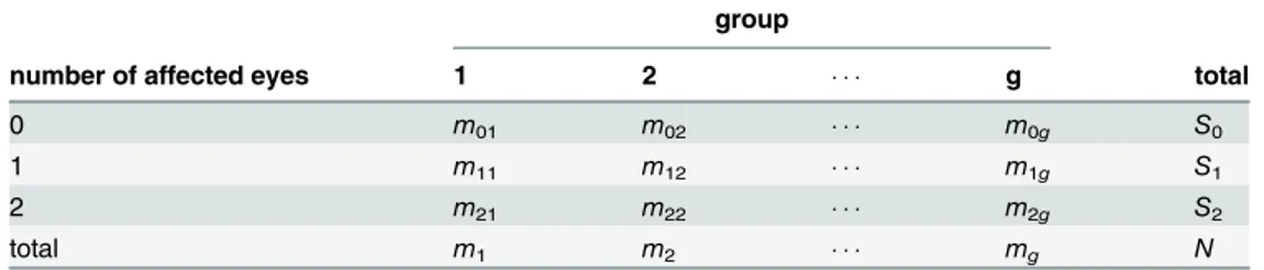
Suppose we wish to compareggroups of individuals from an ophthalmologic study withmi in-dividuals in theith group,i= 1,. . .,g;N=∑_{mitotal subjects (Table 1). LetZijk= 1 if thekth eye}

ofjth individual in theith group has a response at the end of the study, and 0 otherwise,i= 1, . . .,g,j= 1,. . .,mi,k= 1, 2. Letmlidenote the number of subjects who has exactlylresponses in theith group, andSlbe the number of subjects who has exactlylresponses (e.g., affected eyes)

Sl¼ X

g

i¼1

mli;l¼0;1;2:

A parametric model proposed by [5] is given as

PrðZijk¼1Þ ¼pi;PrðZijk¼1jZij;3 k¼1Þ ¼Rpi; ð1Þ

i= 1,. . .,g,j= 0,. . .,mi,k= 1, 2 for some positiveR. The constantRis a measure of depen-dence between two eyes of the same person. IfR= 1, the two eyes from the same patient are completely independent. IfRπi= 1, the eyes of each patient in thei-th group are completely de-pendent. TheRsatisfies 0<R1/a, ifa1/2; (2−_1/a)/aR1/a, ifa>1/2; wherea= max{πi,i= 1,. . .,g}. From the conditional probability inEq (1), it is easy to show that the

Table 1. Frequencies of the number of affected eyes for persons inggroups. group

number of affected eyes 1 2 g total

0 m01 m02 m0g S0

1 m11 m12 m1g S1

2 m21 m22 m2g S2

total m1 m2 mg N

correlation between two eyes is

r_i¼corrðZij1;Zij2Þ ¼

p_i

1 p_iðR 1Þ;i¼1; . . .;g: ð2Þ

We wish to test whether the response rates of theggroups are identical. The hypotheses are given as

H0:p1¼ ¼pg¼p

against

H1:some of thepiare unequal:

Based on the observed dataM~ ¼ ðm01; ;m0g;m11; ;m1g;m21; ;m2gÞ, the

corre-sponding log-likelihood can be expressed as

lðp1;. . .;pg;RÞ ¼ X

g

i¼1

½m0ilogðRpi 2 ₂

p_iþ1Þ þm1ilogð2pið1 RpiÞÞ þm2ilogðRp 2 iފ:

Differentiatingl(π1,. . .,πg;R) with respect to parametersπ1,. . .,πgandRyields

@l

@p_i ¼

2m2i

p_i þ

ð2Rp_i 2Þm0i

Rp_i2 _2p iþ1

þð4Rpi 2Þm1i

2p_iðRp_i 1Þ ;i¼1;. . .;g ð3Þ

@l

@R¼

Xg

i¼1

m2i

R þ

p_i2_m 0i

Rp_i2 _2p iþ1

þ pim1i

Rp_i 1

ð4Þ

Under the null hypothesisH0:π1= =πg=π, the maximum likelihood estimates ofπand

Rsatisfy

@l

@R¼0and

@l

@p¼

2S2

p þ

ð2Rp 2ÞS0

Rp2 _2pþ1þ

ð4Rp 2ÞS1 2pðRp 1Þ¼0;

A direct algebra calculation results in the MLEs ofp0

isandR

^

p_H0 ¼S1þ2S2 2N

and

^

RH0¼

4NS2

ðS1þ2S2Þ 2:

Denotep^_i;i¼1;. . .;gandR^as the maximum likelihood estimate ofπi,i= 1,. . .,gandR,

respectively.p^_i;i¼1;. . .;gandR^are the solution of the following equations

@l

@p_i ¼0;i¼1;. . .;g; @l

@R¼0:

There is no closed form solution and it has to be solved iteratively. We can simplify the formula inEq (3)as the following 3rd order polynomial (fori= 1,. . .,g)

p3 i

4m0iþ5m1iþ6m2i 2Rmi

p2 i þ

m0iþ ð1þRÞm1iþ ð2þRÞm2i

R2_m i

p_i m1iþ2m2i

2R2_m i

The (t+ 1)th update forπican be directly obtained by the real root of the above equation, and Rcan be updated by the Fisher scoring method

Rðtþ1Þ_¼RðtÞ @

2_l

@R2ðp

ðtÞ

1 ;. . .;p

ðtÞ

g ;R

ðtÞ_Þ

1 _@

l

@Rðp

ðtÞ

1 ;. . .;p

ðtÞ

g ;R

ðtÞ_Þ:

See next section for the formula of@2_l

@R2.

Information matrix

@p_i;i¼1;. . .;gand

@l

@Rwith respect toπi,i= 1,. . .,gandRrespectively yields

@2

l

@p2 i

¼ m0ið 2R 2_p2

i þ4Rpiþ2R 4Þ

ðRp2

i 2piþ1Þ 2

2m2i

p2 i

ð2R2_p2

i 2Rpiþ1Þm1i

p2

iðRpi 1Þ

2 ;

@2

l

@p_i@R ¼

m_1i

ðRp_i 1Þ2

2ðp_i 1Þp_im_0i

ðRp_i2 _2p iþ1Þ

2;

i¼1;. . .;g

@2

l

@p_i@p_j ¼ 0;i6¼j;

@2

l

@R2 ¼

S2

R2 Xg

i¼1

p2 i m1i

ðRp_i 1Þ2 Xg

i¼1

p4 i m0i

ðRp2

i 2piþ1Þ 2:

Then we have

Iii ¼ E

@2

l

@p2 i

¼2mið2R 2_p

i 2 _Rp

i

2 _2Rp iþ1Þ

p_iðRp_i2 _2p

iþ1Þð1 RpiÞ

;

Ii;gþ1 ¼ E

@2

l

@p_i@R

¼ 2ð1 RÞpi

2_m i

ðRp_i2 _2p

iþ1Þð1 RpiÞ

;

i¼1;. . .;g

Iij ¼ E

@2

l

@p_i@p_j !

¼0;i6¼j;

Igþ1;gþ1 ¼ E

@2

l

@R2

¼X

g

i¼1

p_i2_m

iðRpi 2piþ1Þ

RðRp_i2 _2p

iþ1Þð1 RpiÞ

:

The (g+ 1) × (g+ 1) information matrix is denoted asI(π1,. . .,πg;R) = (Iij).

Under the null hypothesisH0:π1= =πg=π, it is straightforward but tedious to show

that the inverse of the information matrix can be expressed as

I 1_{ðp;RÞ ¼} p

4_{RðR 1Þ}2

Nð2p2_R2 _p2_{R 2pRþ1Þ}

c1 1 1 d

1 c2 1 1 d

1 1 cg d

d d d d h

2 6 6 6 6 6 6 6 6 6 6 4 3 7 7 7 7 7 7 7 7 7 7 5

where

ci ¼

ðRp2 _{2pþ1Þ ð1 pRÞN} 2p3_{RðR 1Þ}2_m

i

þ1;i¼1;. . .;g;

d ¼ 2p

2_R2 _p2_{R 2pRþ1}

p3_{ðR 1Þ} ;

h ¼ ð2p

2_R2 _p2_{R 2pRþ1Þ}2

p6_{ðR 1Þ}2 :

With the MLEs and information matrix derived, we consider the following test statistics.

Likelihood ratio test (

T

)

The likelihood ratio (LR) test is given by

TLR ¼2½lð^p1;. . .;^pg; ^RÞ lð^pH0;. . .;p^H0; ^RH0ފ:

Under the null hypothesis,TLRis asymptotically distributed as a chi-square distribution withg

−_{1 degrees of freedom.}

Wald-type test (

T

)

The null hypothesisH0:π1= =πgcan be alternatively expressed asCβT= 0 whereβ= (π1, ,πg,R) and

C¼

1 1 0

1 1 0

. . .

. . .

.. .

1 1 0

2

6 6 6 6 6 6 6 4

3

7 7 7 7 7 7 7 5

g 1;g

:

Wald-type test statistic (TW) for testingH0can be expressed as

TW¼ ðbCTÞðCI 1_CT_Þ 1

ðCbTÞjb¼ ðp^1;. . .;p^g;R^Þ;

whereIis the Fisher information matrix for andTWis asymptotically distributed as a chi-square distribution withg−_{1 degrees of freedom.TWcan be simplified as}

TW¼ Pg

i;j¼1^pip^jDij Pg

k¼1ðb 2 k hakÞ

where

Dij ¼ (

ðb2 i haiÞ

P

k6¼iakþaið P

k6¼ibiÞ 2

; if i¼j;

biaj P

k6¼jbkþbjai P

k6¼i bk haiaj bibj P

k6¼i;jak; if i6¼j;

ak¼

2mkð2^R 2_p^2

k R^p^ 2

k 2^Rp^kþ1Þ ^

p_kð_R^2_p^3 k 3^Rp^

2

kþR^^pkþ2^pk 1Þ

;

bk¼

2mkð1 R^Þp^ 2 k ^

R2_p^3 k 3^Rp^

2

kþR^p^kþ2^pk 1

;

h¼X

g

i¼1

mi

^

p4 i 1 2^p_iþ_R^_p^2

i

þp^

2 i ^

R þ

2^p3 i 1 R^p^_i

" #

:

Other multivariate tests ofπ’s can be similarly done by choosing the correspondingCmatrix

in the above statistic. Further, a Wald-type test statistic for testingH0a:πi=πjvsH1a:πi6¼πj,i

6¼jcan be given by

TWaði;jÞ ¼ ðbcTÞðcI 1_cT_Þ 1

ðcbTÞjb¼ ðp^1;. . .;p^g;R^Þ;

wherec= (0,. . ., 1,. . .,−_1,. . ., 0) with 1 in theith element and−_{1 in thejth element.TWais}

as-ymptotically distributed as a chi-square distribution with 1 degree of freedom.TWa(i,j) can be simplified as

TWaði;jÞ ¼

aiajðp^i p^jÞ 2

ðPg k¼1ðb

2

k=akÞ hÞ

ðaiþajÞð Pg

k6¼i;jðb2k=akÞ hÞ þ ðbiþbjÞ 2:

Score test (

T

)

The score test statisticTSCis given by

T2

SC¼UIðp;RÞ 1

UT_jp

1 ¼ ¼pg¼p^H0;R¼

^

RH0

where

U ¼ @l @p₁;. . .;

@l

@p_g;0 !

and see (Eq 5) for the formula of the inverse of the information matrixI(π,R)−1.

It can be simplified as

T2 SC¼

X g

k¼1

NðS2

1m0k S0S1ðm1kþ2m2kÞ þ2S0S2m1kÞ 2

S0S1ðS 3 1þS0S

2 1þ4S0S

2 2Þmk

ð6Þ

after lengthy algebra calculations.T2

SCis asymptotically distributed as a chi-square distribution

withg−_{1 degree of freedom.}

Remark1. One limitation of the score statistic is that it cannot be computed ifS0= 0 orS1=

Remark2. [1] derived a score testTSCforg= 2 as

TSC¼

N½S0S1ðm11þ2m21Þ m01S 2

1 2m11S0S2Š ffiffiffiffiffiffiffiffiffiffiffiffiffiffiffiffiffiffiffiffiffiffiffiffiffiffiffiffiffiffiffiffiffiffiffiffiffiffiffiffiffiffiffiffiffiffiffiffiffiffiffiffiffiffiffiffiffiffiffi

m1m2S0S1½S21ðS0þS1Þ þ4S0S22Š

p ;

which is equivalent to (Eq 6).

Monte Carlo simulation studies

We now investigate the performance of proposed statistics and testing procedures discussed in the previous section. First, we investigate the behavior of the type I error rates of various proce-dures forg= 2,3,4,5; sample sizem1= =mg= 20, 40, 60, 80 and 100;π1= =πg=π0= 0.5

(0.1)0.8; andR= 1 +ρ(1−π0)/π0whereρ= 0.4(0.1)0.6. An imbalanced sample setting is also

considered. In each configuration, 50,000 replications are generated based on the null hypothe-sis, and empirical type I error rates are computed asthe number of rejections/50000. The results are presented inTable 2. Following [1], we calculated the ratio of empirical type I error rate to the nominal type I error rate. A test is said to be liberal if the ratio is greater than 1.2 (i.e.,>6% forα= 5%), conservative if the ratio is less than 0.8 (i.e.,<4%), and robust if the ratio is be-tween 0.8 and 1.2.

Generally, score testsT2

SCproduce satisfactory type I error controls for any configuration

while LR tests and Wald tests are liberal, especially for small samples and larger numbers of groups (g). Wheng>2, Wald tests are more liberal than LR tests and these tests get closer when sample size becomes larger.

LR tests and Wald-type tests are extremely liberal for a small sample size (i.e.,m= 20), and their actual sizes inflate with the increase of the correlation coefficient (i.e.,ρ).

Next, we evaluate the power performance of proposed methods. We consider the alternative hypotheses withH1:π= (0.25, 0.4), (0.25, 0.325, 0,4), and (0.25, 0.3, 0.35, 0.4) forg= 2, 3, and

4, respectively.Ris chosen as 1, 1.5, and 2.0 and sample sizem1= =mg= 20, 40, 60, 80 and 100. Ronser’s statisticTis also considered in the simulation studies and the results are pre-sented inTable 3.

Based on the simulation results, LR and Wald tests are generally more powerful than score tests and Ronser’sTgenerally has less power. However, power of LR and Wald tests is often overestimated in small sample size due to the inflated type I error rates from these tests being observed (seeTable 2). For moderate or large sample sizes, the powers of the three proposed methods are close. Overall, the score test is highly recommended as it has reasonable power with satisfactory type I error control.

Examples

We first reanalyze the data presented by [5] to illustrate the newly proposed methods. The data consists of 218 persons aged 20–39 with retinitis pigmentosa (RP) who were seen at Massachu-setts Eye and Ear Infirmary. They were classified into four genetic types, namely, autosomal dominant RP (DOM), autosomal recessive RP (AR), sex-linked RP (SL), and isolate RP (ISO). The differences between these four groups on the Snellen visual acuity (VA) were assessed. An eye was considered affected if VA was 20/50 or worse, and normal if VA was 20/40 or better. The sample used for this analysis consists of 216 persons out of the sample of 218 persons each of whom had complete information for VA on both eyes (Table 4).

An overall significant difference between the proportions of affected eyes in the four groups is from 0.0769 to 0.1173 based on proposed methods and 0.010 on Rosner’s statisticT

Table 2. The type I error rates (percent) of various procedures underH0:π1= =πg=π0atα= 0.05 based on 50,000 replicates.

m π0 ρ g= 2 g= 3 g= 4 g= 5

T2

LR T

2

W T

2

SC T

2

LR T

2

W T

2

SC T

2

LR T

2

W T

2

SC T

2

LR T

2

W T

2

SC 20 0.5 0.4 6.70 6.63 5.39 6.95 8.09 5.06 7.10 9.64 4.99 7.19 10.66 5.05

0.5 6.70 5.76 5.34 7.11 7.66 5.10 7.34 9.48 5.01 7.34 10.81 4.82 0.6 7.11 4.86 5.35 7.27 6.94 4.80 7.72 9.51 4.79 8.19 11.97 4.92 0.6 0.4 6.63 6.51 5.25 6.80 8.18 5.16 7.05 9.42 5.15 6.87 10.44 4.80 0.5 6.64 5.57 5.32 6.82 7.14 4.95 6.96 8.93 4.82 7.38 10.45 4.92 0.6 7.18 4.58 5.37 7.34 6.95 4.91 7.64 9.29 4.89 7.80 11.54 4.85 0.7 0.4 6.46 6.28 4.76 6.79 7.96 5.05 6.85 9.28 4.92 6.99 10.55 4.77 0.5 6.90 5.58 5.11 6.89 7.23 4.90 7.30 9.06 4.77 7.64 10.98 4.91 0.6 7.46 4.43 5.02 7.72 6.94 4.80 7.97 10.36 4.73 8.42 13.80 4.92 0.8 0.4 6.76 6.51 4.94 7.26 8.35 4.85 7.49 10.37 4.81 7.71 12.15 4.75 0.5 7.58 5.45 4.99 7.92 7.89 4.78 8.04 11.50 4.72 8.24 14.92 4.65 0.6 7.81 4.00 4.37 8.31 6.94 4.46 8.15 11.87 4.42 8.28 17.56 4.52

40 0.5 0.4 5.72 5.61 5.07 6.00 6.42 5.16 5.86 7.01 4.97 6.00 7.66 5.03

0.5 5.71 5.11 5.15 5.84 5.89 4.98 5.90 6.80 4.91 6.11 7.55 4.92

0.6 5.76 4.66 5.13 5.84 5.48 4.98 6.12 6.62 4.97 6.20 7.45 5.02

0.6 0.4 5.58 5.48 4.98 5.72 6.08 5.05 5.83 6.90 4.98 5.87 7.48 4.99

0.5 5.74 5.13 5.14 5.82 5.83 5.03 6.04 6.73 5.18 6.16 7.57 5.13

0.6 5.84 4.73 5.19 5.79 5.37 5.00 5.98 6.49 4.94 6.05 7.43 4.97

0.7 0.4 5.62 5.41 5.03 5.84 6.11 5.13 5.58 6.42 4.85 5.71 7.30 4.89

0.5 5.59 4.94 4.96 5.88 5.79 5.21 5.86 6.65 5.05 5.69 7.28 4.89

0.6 5.74 4.56 5.00 5.73 5.60 4.88 6.01 6.76 5.00 6.08 7.59 4.97

0.8 0.4 5.76 5.33 5.30 5.85 6.16 4.99 5.98 7.19 5.10 6.00 8.00 5.04

0.5 5.58 4.63 4.97 5.68 5.78 4.76 5.81 6.87 4.68 6.00 7.79 4.92

0.6 5.85 4.44 4.91 5.91 5.71 4.67 6.20 7.23 4.77 6.43 8.51 4.71

60 0.5 0.4 5.39 5.20 4.94 5.67 6.02 5.06 5.60 6.27 4.95 5.62 6.77 4.91

0.5 5.57 5.10 5.11 5.85 5.83 5.23 5.75 6.28 5.02 5.74 6.59 4.99

0.6 5.58 4.67 5.06 5.60 5.28 5.02 5.84 6.08 5.15 5.51 6.39 4.79

0.6 0.4 5.57 5.46 5.19 5.57 5.77 5.06 5.38 6.09 4.86 5.80 6.75 5.14

0.5 5.36 4.90 4.97 5.42 5.39 5.01 5.55 5.85 4.94 5.57 6.39 4.91

0.6 5.56 4.79 5.21 5.56 5.33 4.98 5.52 5.78 4.93 5.69 6.62 4.95

0.7 0.4 5.46 5.24 5.09 5.51 5.62 5.10 5.60 6.23 5.08 5.44 6.47 4.85

0.5 5.44 4.99 5.10 5.54 5.51 5.08 5.48 6.02 4.97 5.47 6.55 4.85

0.6 5.42 4.70 5.04 5.32 5.14 4.84 5.50 5.82 4.91 5.47 6.57 4.82

0.8 0.4 5.41 5.05 5.07 5.52 5.69 5.01 5.47 6.19 4.94 5.50 6.76 4.97

0.5 5.42 4.79 5.04 5.67 5.58 5.19 5.61 6.14 4.98 5.53 6.91 4.80

0.6 5.36 4.56 4.87 5.76 5.59 5.08 5.78 6.54 4.88 5.81 7.33 4.94

80 0.5 0.4 5.29 5.17 4.95 5.56 5.75 5.12 5.61 6.21 5.13 5.50 6.32 5.00

0.5 5.25 4.88 4.91 5.34 5.37 5.02 5.43 5.75 4.90 5.53 6.14 4.96

0.6 5.34 4.72 5.05 5.49 5.26 5.08 5.50 5.70 4.93 5.59 6.09 5.04

0.6 0.4 5.46 5.34 5.23 5.41 5.51 4.99 5.25 5.66 4.82 5.38 6.10 4.98

0.5 5.32 4.91 5.02 5.26 5.25 4.96 5.47 5.77 5.16 5.37 5.98 4.97

0.6 5.31 4.75 4.98 5.35 5.12 5.00 5.59 5.81 5.15 5.35 6.04 4.92

0.7 0.4 4.99 4.78 4.75 5.30 5.41 4.97 5.30 5.74 4.92 5.45 6.24 4.98

0.5 5.35 4.93 5.13 5.36 5.26 5.06 5.58 5.96 5.16 5.37 6.00 4.90

0.6 5.38 4.83 5.13 5.41 5.38 5.03 5.39 5.83 4.91 5.42 6.01 4.86

0.8 0.4 5.32 4.97 5.08 5.47 5.51 5.09 5.35 5.81 4.97 5.40 6.22 4.96

The maximum likelihood estimates and pairwise comparisons based on Wald-type test TWa(i,j) are shown inTable 6. It shows a significant difference between DOM and AR (p = 0.0207).

Another example was a recent study from a cross-sectional, population-based sample in Iran assessing the prevalence of avoidable blindness [11]. Nearly 3000 persons were examined and blindness was assessed for seven age groups (Table 7). Test statisticsT2

LR¼134:7,

T2

W¼89:1,T 2

SC¼161:1, andT= 202.0 consistently show the significant age differences

(p-values<0.0001), and MLER^¼3:35(r^_i ¼ p^_i

1 ^p_iðR^ 1Þare from 0.05 to 0.59) shows positive

correlations between eyes for the same person.

Concluding remarks

In this article, we investigated three procedures for testing the homogeneity of correlated data with a cluster size of two. We derived the maximum likelihood estimate algorithm by utilizing Table 2. (Continued)

m π0 ρ g= 2 g= 3 g= 4 g= 5

T2

LR T

2

W T

2

SC T

2

LR T

2

W T

2

SC T

2

LR T

2

W T

2

SC T

2

LR T

2

W T

2

SC

0.5 5.04 4.61 4.83 5.51 5.44 5.16 5.60 6.05 5.14 5.27 6.22 4.86

0.6 5.19 4.64 4.92 5.39 5.40 4.86 5.46 6.00 4.90 5.49 6.52 4.86

100 0.5 0.4 5.23 5.09 4.94 5.27 5.38 4.98 5.34 5.81 4.98 5.21 5.90 4.72

0.5 5.41 5.13 5.17 5.40 5.44 5.01 5.32 5.64 4.98 5.44 5.96 4.99

0.6 5.39 4.85 5.16 5.45 5.25 5.14 5.28 5.38 4.83 5.47 5.78 4.95

0.6 0.4 5.33 5.23 5.13 5.42 5.63 5.18 5.46 5.79 5.15 5.17 5.82 4.83

0.5 5.11 4.85 4.91 5.40 5.29 5.02 5.39 5.62 5.07 5.13 5.66 4.79

0.6 5.26 4.87 5.07 5.48 5.23 5.21 5.37 5.48 4.96 5.09 5.53 4.76

0.7 0.4 5.37 5.16 5.18 5.15 5.23 4.85 5.44 5.74 5.05 5.35 5.87 5.08

0.5 5.17 4.90 5.00 5.15 5.08 4.91 5.16 5.47 4.86 5.28 5.83 4.96

0.6 5.50 5.06 5.29 5.38 5.27 5.08 5.36 5.61 4.99 5.30 5.87 4.93

0.8 0.4 5.33 5.09 5.09 5.04 5.12 4.78 5.29 5.72 4.91 5.31 5.93 4.95

0.5 5.16 4.79 4.93 5.23 5.21 4.97 5.45 5.84 5.03 5.38 6.21 4.88

0.6 5.18 4.72 4.88 5.38 5.31 4.96 5.62 6.04 5.19 5.38 6.35 4.85

* 0.5 0.4 6.32 6.87 5.30 6.14 7.42 4.92 6.62 8.69 5.15 6.29 9.33 4.81

0.5 6.44 6.54 5.29 6.49 7.30 5.05 6.60 8.47 4.93 6.62 9.50 4.86

0.6 6.54 6.07 5.13 6.58 7.11 4.93 6.88 8.66 4.91 6.88 9.76 4.95

0.6 0.4 5.91 6.42 5.07 6.12 7.34 4.98 6.33 8.40 5.04 6.40 9.31 5.10

0.5 6.00 6.16 4.95 6.48 7.39 5.19 6.61 8.31 5.17 6.32 9.10 4.77

0.6 6.16 5.99 4.85 6.52 6.91 4.97 7.15 8.54 5.06 6.91 9.69 4.92

0.7 0.4 6.00 6.44 5.13 6.17 7.36 5.09 6.19 8.30 4.88 6.26 9.26 4.82

0.5 6.26 6.24 5.19 6.30 7.25 4.91 6.50 8.20 4.83 6.75 9.48 5.11

0.6 6.56 6.15 5.04 6.75 7.28 4.90 6.99 8.90 4.77 6.58 9.90 4.67

0.8 0.4 6.20 6.74 5.01 6.48 7.60 5.07 6.78 9.04 4.92 6.71 9.93 4.81

0.5 6.77 6.71 5.04 6.69 7.65 4.72 7.09 9.59 4.80 6.72 10.54 4.62 0.6 7.16 7.08 4.63 7.50 9.41 4.83 7.75 12.24 4.78 7.36 14.32 4.60 *unequal sample sizes: (m1,. . .,mg) = (20,40), (20,30,40), (20, 25, 30, 35), (20,25,30,35,40) forg= 2,3,4,5, respectively.

Table 3. The power (percent) of various procedures atα= 0.05 based on 50,000 replicates.

m R g= 2 g= 3 g= 4

T2

SC T

2

LR T

2

W T T

2

SC T

2

LR T

2

W T T

2

SC T

2

LR T

2

W T

20 1.0 29.5 31.7 33.5 30.2 22.1 24.8 28.7 22.7 20.6 23.5 28.5 20.9

1.5 24.7 29.2 29.9 24.5 18.7 23.2 26.0 18.7 17.4 22.1 26.6 16.8

2.0 30.0 36.4 29.8 21.3 23.6 30.8 27.4 16.1 21.9 29.4 29.4 14.8

40 1.0 52.2 53.5 54.9 52.8 41.9 43.6 46.1 42.3 39.9 41.7 44.7 40.1

1.5 45.6 48.7 49.3 44.1 35.9 39.5 41.3 34.2 34.4 37.8 40.7 32.3

2.0 55.9 60.0 55.6 37.6 45.8 50.6 48.3 29.1 43.7 48.7 48.2 27.2

60 1.0 69.8 70.6 71.5 70.2 59.4 60.6 62.3 60.0 57.5 58.8 60.9 57.8

1.5 62.7 64.8 65.3 60.1 52.3 54.8 56.3 49.5 50.4 53.1 55.2 47.3

2.0 74.3 76.6 74.4 52.6 64.8 68.2 66.8 42.0 63.4 66.9 66.2 40.2

80 1.0 81.7 82.2 82.7 82.1 72.9 73.7 74.7 73.2 71.4 72.2 73.6 71.5

1.5 75.9 77.2 77.6 72.7 65.8 67.6 68.7 62.3 64.7 66.6 68.0 61.0

2.0 86.1 87.2 86.1 64.5 78.4 80.6 79.7 53.8 78.0 80.2 79.9 52.3

100 1.0 89.4 89.6 89.9 89.6 82.6 83.1 83.7 82.7 82.0 82.5 83.4 82.1

1.5 84.8 85.6 85.9 82.1 76.4 77.7 78.5 73.0 75.5 76.9 77.9 71.6

2.0 92.8 93.4 92.8 74.3 87.4 88.9 88.4 64.6 87.4 88.8 88.6 63.0

H1: π= (0.25, 0.4) (0.25, 0.325, 0,4) (0.25, 0.3, 0.35, 0.4)

Note:Tis the test statistic [5].

doi:10.1371/journal.pone.0124337.t003

Table 4. Distribution of the number of affected eyes for persons in each genetic type [5]. genetic type

number of affected eyes DOM AR SL ISO

0 15 7 3 67

1 6 5 2 24

2 7 9 14 57

doi:10.1371/journal.pone.0124337.t004

Table 5. Statistic and p-value for comparing VA for different genetic types of RP.

method T2

LR T

2

W T

2

SC T

statistic 5.8862 6.2966 6.8475 11.36

p-value 0.1173 0.0980 0.0769 0.010

the root of third order polynomial equations. The Fisher scoring method is usually criticized for converging slowly, especially when the number of parameters is large (e.g.gis large). How-ever, the algorithm derived in this paper is very efficient. This is because onlyRis updated by Fisher scoring iterations, andπi,i= 1,. . .,gare the roots of third order polynomials, a closed

form solution.

Simulation results showed that the proposed approach (score test) has satisfactory type I error control and reasonable power, regardless of number of groups, sample size, or parameter configurations. On the other hand, the LR test and Wald test have inflated type I error in small sample size. When sample size becomes larger, the three test procedures get closer.

For binary correlated data, there are alternative ways to solve the MLE iteratively or perform hypothesis testing by model-based methods, e.g., GENMOD or GLIMMIX in SAS. However, neither iterative version of test statistics nor model-based method provides the explicit form of the test statistic. The explicit form of the test statistic in our proposed method is useful not only for its simplicity, but also for further development of the exact test. For example, in small sam-ple situation, an exact test may overcome the inflated type I error rate and thus is highly desir-able. To perform exact test, it will requires extensive calculations which makes it nearly impossible using iterative versions of test statistics or model-based methods.

To overcome inflated type I error control in asymptotic tests, [10] and [12] considered exact tests forg= 2. We consider the exact tests forg>2 as interesting future work.

A user-friendly web-based calculator, including model estimations, hypothesis testings, and simulations, is available from the corresponding author upon request.

Table 6. Wald-type test results comparing VA for different genetic types of RP. Groupi MLE^_p^

i Standard Error Comparison group

DOM AR SL ISO

DOM 0.3930 0.0041 – -0.0868 (p= 0.3116) -0.1698 (p= 0.0207) -0.1001 (p= 0.1363)

AR 0.4798 0.0039 – -0.0830 (p= 0.2135 -0.0132 (p= 0.8284)

SL 0.5628 0.0022 – 0.0697 (p= 0.0748)

ISO 0.4931 0.0011 –

^

R^

¼1:6639

doi:10.1371/journal.pone.0124337.t006

Table 7. Prevalence of avoidable blindness from a sample population in Iran [11].

Age Group Blindness Sample Prevalence MLE

None Unilateral Bilaterial

50–54 yrs 964 23 2 0.014 0.014

55–59 yrs 541 17 8 0.029 0.030

60–64 yrs 469 18 4 0.026 0.027

65–69 yrs 257 16 5 0.047 0.048

70–74 yrs 242 32 3 0.069 0.067

75–79 yrs 127 30 9 0.145 0.134

80+ yrs 104 29 10 0.171 0.149

Acknowledgments

The authors thank the associate editor and three referees for constructive comments and sug-gestions which improve the presentation of the paper.

Author Contributions

Conceived and designed the experiments: CM GS. Performed the experiments: CM. Analyzed the data: CM. Contributed reagents/materials/analysis tools: CM GS. Wrote the paper: CM GS SL.

References

1. Tang NS, Tang ML, Qiu SF. Testing the equality of proportions for correlated otolaryngologic data.

Computational Statistics & Data Analysis, 52(7):3719–3729, March 2008. doi:10.1016/j.csda.2007.12.

017

2. Simon R, Wittes RE, Ellenberg SS. Randomized phase II clinical trials.Cancer treatment reports, 69 (12):1375–1381, December 1985. PMID:4075313

3. Wilding GE, Shan G, Hutson AD. Exact two-stage designs for phase II activity trials with rank-based endpoints.Contemporary Clinical Trials, 2011.

4. Donner A. Cluster randomization trials in epidemiology: theory and application.Journal of Statistical Planning and Inference, 42(1–2):37–56, November 1994. doi:10.1016/0378-3758(94)90188-0

5. Rosner B. Statistical methods in ophthalmology: an adjustment for the intraclass correlation between eyes.Biometrics, 38(1):105–114, March 1982. doi:10.2307/2530293PMID:7082754

6. Dallal GE. Paired Bernoulli trials.Biometrics 44, 253–257, 1988. doi:10.2307/2531913PMID:

3358992

7. Rosner B, Milton RC. Significance testing for correlated binary outcome data.Biometrics 44, 505–512,

1988. doi:10.2307/2531863PMID:3390508

8. Donner A. Statistical methods in ophthalmology: An adjusted chi-square approach.Biometrics 45, 605–611. doi:10.2307/2531501PMID:2765640

9. Bodian CA. Intraclass correlation for two-by-two tables under three sampling designs.Biometrics50, 183–193, 1994. doi:10.2307/2533208PMID:8086601

10. Tang ML, Tang NS, Rosner B. Statistical inference for correlated data in ophthalmologic studies. Statis-tics in Medicine 25, 2771–2783, 2006. doi:10.1002/sim.2425PMID:16381067

11. Rajavi Z, Katibeh M, Ziaei H, Fardesmaeilpour N, Sehat M, Ahmadieh H, et al. Rapid assessment of avoidable blindness in Iran,Ophthalmology118, 1812–18, 2011. doi:10.1016/j.ophtha.2011.01.049

PMID:21571371

12. Shan G, Ma CX. Exact Methods for Testing the Equality of Proportions for Binary Clustered Data From Otolaryngologic Studies.Statistics in Biopharmaceutical Research, 6, 115–122, 2014. doi:10.1080/