autoinhibition: Stability of dynamic states
Stevan Maćešić1, Željko Čupić2, Ljiljana Kolar-Anić1
1
University of Belgrade, Faculty of Physical Chemistry, Belgrade, Serbia
2
University of Belgrade, Institute of Chemistry, Technology and Metallurgy, Department of Catalysis and Chemical Engineering, Belgrade, Serbia
Abstract
Self-regulation, achieved through positive (autocatalytic) or negative (autoinhibitory) feed-back is commonly encountered in natural, technological and economic systems. The dyna-mic behavior of such systems is often complex and cannot be easily predicted, necessi-tating mathematical modelling and theoretical analyses. The aim of this work is to analyze the dynamics of a minimal model system with autocatalytic and autoinhibitory steps coupled through the same species, in order to understand under which critical condition the sys-tem loses stability and passes through an Andronov-Hopf bifurcation. The analysis used was improved stoichiometric network analysis (SNA) in combination with bifurcation and sensitivity analysis.
Keywords: Nonlinear dynamics; stoichiometric network analysis; autocatalysis; HPA system; Andronov–Hopf bifurcation.
SCIENTIFIC PAPER
UDC 544.474:544:517.9
Hem. Ind.66 (5) 637–646 (2012)
doi: 10.2298/HEMIND120210034M
Available online at the Journal website: http://www.ache.org.rs/HI/
Autocatalysis and autoinhibition often exist to-gether in complex dynamical systems that exhibit self-regulation, but the feedback is not necessarily achieved through the same intermediate species. We analyze here a low-dimensional reaction model where positive and negative feedback loops are coupled, occurring through the same species. In order to understand how the stability of this system is affected by the concen-trations of other reactive species and the kinetic rate constants, we have generated MATLAB routines for im-proved stoichiometric network analysis (SNA) [1]. We use stability and bifurcation analyses for a detailed dis-cussion of dynamic states.
THE MODEL
The Model (R1)–(R9) (Table 1), consists of four reac-tion species (B, M, A and G) and nine reacreac-tions cha-racterized by kinetic rate constants ki (i = 1, 2,...,9).
It contains one positive (R6) and one negative (R7) feedback loop that are coupled through the same intermediate (G). These two reactions are important for oscillatory behavior of the systems [2,3].
Positive/negative feedback coupling can be found in many natural systems, such as the hypothalamo-hypo-fizo adrenal (HPA) axis [4].
The dynamics of the Model (R1)–(R9)can be repre-sented by a set of ordinary differential kinetic equations:
Correspondence: S. Maćešić, University of Belgrade, Faculty of Phy-sical Chemistry, Studentski trg 12-16, 11000 Belgrade, Serbia. E-mail: [email protected]
Paper received: 10 February, 2012 Paper accepted: 20 March, 2012
1 3
d d
b
k k b
t
= −
(1)
2
2 5 7
d d
m
k k a k mg
t
= + −
2
3 4 5 6 8
d d
a
k b k a k a k ag k a
t
= − − − −
2 2
4 6 7 9
d d
g
k a k ag k mg k g
t
= + − −
where a, b, g, and m are concentrations of inter-mediate reaction species A, B, G and M, respectively; t
is the time. Having four variables, this model cannot be analyzed by standard mathematical procedure appro-priate for two or three variables, requiring improved stoichiometric network analysis [5].
Table 1. Model (R1)–(R9) which consists nine reactions [(R1)–(R9)]
Reaction Rate constant
1 k
⎯⎯→ B 8 1
1 1.83 10 min
k = × − − (R1)
2 k
⎯⎯→ M 11 1
2
k 6.09 10− min−
= × (R2)
B ⎯⎯k3→ A −
= 1
3 1.83 min
k (R3)
A ⎯⎯k4→ G − −
= × 2 1
4 3.60 10 min
k (R4)
A ⎯⎯k5→ M 4 1
5 2.88 10 min
− −
= ×
k (R5)
A + 2G ⎯⎯k6→ 3G 14 1 -2 6
6 1.26 10 min mol dm
k = × − (R6)
M + 2G ⎯⎯k7→ G 12 1 -2 6
7 7.05 10 min mol dm
k = × − (R
7)
A ⎯⎯k8→ P
1 k8 =5.35 10 min× −2 −1 (R8) G ⎯⎯k9→ P
Stoichiometric network analysis of considered model In SNA [5–7], the kinetic equations of any stoichio-metric model presented by a set of differential kinetic equations such as (1) are written in the matrix form:
= ×
c S v
(2)where ċis the time derivative of the m×1 concentration vector c comprising the change in concentrations of m
independent intermediate species, known as internal ones in SNA. S is the stoichiometric matrix and v is the so-called reaction or flux vector with reaction rates as components. The stoichiometric matrix S is an m×n
matrix where n is the number of reactions in the reac-tion network (in the model considered m = 4 and n = 9). The Sik element of the stoichiometric matrix corres-ponds to the stoichiometric coefficient of reactive spe-cies i in reaction (Rk) corresponding to column k and row i. The reaction vector v is a 1×n vector whose elements describe the reaction rates.
Using the matrix representation given in Eq. (2), the Model (R1)–(R9) (Table 1) corresponds to the following system of differential equations:
1
2
1 2 3 4 5 6 7 8 9 3
4
5
6
7
8
9 1 0 1 0 0 0 0 0 0
0 1 0 0 1 0 1 0 0 0 0 1 1 1 1 0 1 0 0 0 0 1 0 1 1 0 1
v
v
R R R R R R R R R v
v
c v
v
v
v
v
⋅
−
= − ×
− − − −
− −
(3)
Now, we want to obtain information about the interplay between the concentrations of independent intermediate species and the dynamics of the network as a whole. As a first step, we look for conditions where the network is in a quasi steady state. The rates at a steady state vss are solutions of the relation [4]:
ss
0= ×S v (4)
Equation (4) represents a system of homogenous equations, and we need to find all its positive solutions. The method of finding all positive solutions of Eq. (4) depends on the size of the examined model. For simpler models, Eq. (4) can be solved by hand. How-ever, if the number of reactions is large, solving Eq. (4) becomes much more complex and the only suitable way is to use computer programs based on algorithms developed for this purpose [8–12].
The solutions of Eq. (4), known as extreme currents [5,6], are reaction pathways in steady state. They offer important information about the consistency of the
model, and correlations between individual reactions like mutual exclusion or coupling [13]. The extreme currents Ei are usually presented as the columns (in any order) of a new extreme current matrix E. In the case considered, it is:
1 2 3 4 5 6 7
1
2
3
4
5
6
7
8
9
1 1 1 1 1 2 2 0 0 0 1 1 0 0 1 1 1 1 1 2 2 0 1 0 1 0 1 0 0 0 0 0 0 1 1 0 0 1 0 1 0 1 0 0 0 1 1 1 1 1 0 0 0 0 0 0 0 1 1 0 0 0 0
E E E E E E E R R R R R R R R R
=
E (5)
In any specific steady state, each extreme current contributes to reaction rates with its own, distinct, extent. The contributions of the extreme currents, de-noted as the current rates ji, are given as the com-ponents of the corresponding vector j. Elements of vector j are nonnegative numbers. The basic equation of the SNA gives relation between rates at a steady state vss,k and current rates jk [4]:
ss
v =Ej (6)
Using Eq. (6), the particular reaction step rаte vss,k can be written in the form:
ss,1 1 2 3 4 5 26 27 v =j +j +j +j +j + j + j
(7) ss,2 4 5
v =j +j
ss,3 1 2 3 4 5 26 27 v =j +j +j +j +j + j + j
ss,4 2 4 6 v =j +j +j
ss,5 6 7
v =j +j
ss,6 3 5 7 v = j +j +j
ss,7 4 5 6 7 v =j +j +j +j
ss,8 1
v = j
ss,9 2 3
v = j +j
The next step in our analysis is to examine the stability of a steady state, to find the instability con-dition. The stability analysis of the particular steady states is usually performed on the linearized form of the general equation of motion of a system around the steady state. Namely, when the system is in a steady state little perturbation of the concentrations of inter-mediate species can be given as linear deviation from the steady state concentrations [14]:
ss
We can expand the time derivative of concentration vector c in a Taylor series near a steady state css and keep the leading terms only (see Appendix III):
ss
d( )
d d
d d d
c c
c c
c
t t t
+ Δ Δ
= = =MΔ (9)
The leading term M is a Jacobian matrix, which in SNA has the form:
ss ss
( , ) diag( ) diag( )T
h v = v h
M S K (10)
where diag(h)is a diagonal matrix whose elements hi are the reciprocal of the steady state concentrations of the species i, for i = 1,…,4, and K is the matrix of the order of reactions with its transpose KT
. Hence, the stability is defined by the sign of the real part of the eigenvalues of the Jacobian matrix. A general deri-vation of the Jacobian matrix M is given in references [7] and [14]. For the model under consideration, the matrix K is:
1 2 3 4 5 6 7 8 9 0 0 1 0 0 0 0 0 0 0 0 0 0 0 0 1 0 0 0 0 0 1 1 1 0 1 0 0 0 0 0 0 2 2 0 1
R R R R R R R R R
B M
A G
=
K (11)
According to Eq. (6), Eq (10) can be transformed to the matrix equation:
( , )
diag( ) diag( )
Th j
=
S
j
h
M
E K
(12)The matrix M written as a function of the SNA parameters ji and hi has particular advantages for the stability analysis since these parameters are non-nega-tive, which is an essential feature of the SNA. The steady-state stability is determined by the sign of eigen-values of M, which are the roots λ of the characteristic polynomial [15]:
0
n n i i i
λ α λ −
=
− =
I M (13)
where, for the considered model, n = 4. If the real parts of all eigenvalues are negative, a steady state is stable. If one or more eigenvalues has positive real parts the steady state is unstable. The number of eigenvalues with positive real parts can be determined by the Routh–Hurwitz criterion. According to this criterion, the number of eigenvalues with positive real parts is equal to the number of the sign changes in the Routh array [15]:
3 2 1
1 2 1
1, , , , , n n R
−
Δ Δ Δ
= Δ
Δ Δ Δ
(14)
where Δi, i = 1,…,n, is i-th Hurwitz determinant, defined as the determinant of the leading principal minor of the Hurwitz matrix H, where leading principal minor of di-mension i is matrix constructed from the first i rows and columns of matrix H:
1 3 5 7 2 1
2 4 6 2 2
1 3 5 2 3
2 4 2 4
1 3 2 5
1 0 0 1 0 0
0 0 0 0
n n n n n
n
α α α α α
α α α α
α α α α
α α α
α α α
α −
−
−
−
−
=
H
(15)
Obviously, αi = 0 for i > n. The steady state is stable if all Hurwitz determinants are positive. If there is only one sign change in the Routh array (14), this indicates that only one eigenvalue has positive real part. Such instability occurs when the largest Hurwitz determinant changes its sign keeping all others positive, and this point presents saddle-node bifurcation. From the Hur-witz matrix (15) we can see that the largest HurHur-witz determinant Δn can be written as:
1
n αn n−
Δ = × Δ (16)
Since the sign of the largest Hurwitz determinant is in this case determined by the sign of the largest coefficient of the characteristic polynomial αn, the sad-dle-node bifurcation can be identified from [15]:
αn = 0 (17)
The Hurwitz matrix gives us also the condition for appearance of the Andronow–Hopf bifurcation, which is of great importance because it is the source of oscil-lations in the system. The Andronow–Hopf bifurcation is a local bifurcation in which the dynamical system loses stability as a pair of two complex conjugate eigen-values cross the imaginary axis. This bifurcation indi-cates an appearance or disappearance of periodic be-havior. The Andronow–Hopf bifurcation occurs when [15,16]:
Δn–1 = 0 (18)
For considered model where n = 4, the Hurwitz mat-rix is:
1 3 2 4 1 3
2 4 0 0
1 0
0 0
0 1 α α
α α
α α
α α
=
H (19)
1 3
2 2
3 2 4 1 2 3 3 4 1
1 3 0
1 0
0 α α
α α α α α α α α
α α
Δ = = − − =
(20)
Application of an instability condition obtained by this method becomes limited by the number of inde-pendent internal species and it is often very difficult to be determined by the classical procedure, but this me-thod is convenient for a numerical evaluation of sta-bility of steady state. A much simpler method to exa-mine the steady-state stability is the use of the matrix of current rates V(j), where:
( )=j − diag( )j T
V S E K (21)
The steady state is considered to be unstable if there is at least one negative diagonal minor of V(j).[6] Although it is an approximation, this criterion often gives satisfactory results. The matrix V(j) for the model considered is:
We examined all diagonal minors and detected those with negative terms, since only these minors can be negative. They are negative when the polynomial obtained from the corresponding determinant is nega-tive. The calculated polynomials have to be compared between one another, the core of instability must be recognized, and the essential one ought to be selected. The aim is to find the polynomial with less possible order. Such obtained polynomials are expressed as a function of ji. In the case considered the selected poly-nomial is:
2 3 24 26 0
j −j + j + j < (23)
However, working with parameters ji is not prac-tical, because they do not have unique solutions, so a much better way is to transform them into rate velo-cities. [1] Linear relations between ji and vss,i can be found from matrix E and Eq. (6), and they are given in Eq. (7). After the transformation, the condition that is critical for the existence of periodic behavior is:
ss,2 ss,4 ss,5 ss,6
v +v +v <v (24)
Equation (24) gives the critical condition, which needs to be fulfilled for periodic temporal evolution of intermediate species that are involved in dynamics of HPA system model, for rate constants given in Table 1.
To determine which diagonal minors with negative terms are the most important for the existence of pe-riodic behavior, it is necessary to perform comparative
analysis with experiments and the numerical simula-tions. These analyses allow us to determine which terms in the polynomial obtained from corresponding determinant are dominant.
Numerical analysis of considered model
Using SNA we can obtain very important infor-mation about the steady-state stability, interaction between reaction species in a steady state, and pos-sible reaction routes. However, this method does not give detailed information about the dynamics of the system, such as type of the oscillations together with their amplitudes and periods. To obtain such infor-mation it is necessary to use additional methods of nu-merical and sensitivity analyses, and nunu-merical inte-gration of a system of ordinary differential equations. However, we had to adapt them in such a manner that they can use main results of SNA. For this purpose we developed corresponding computer programs in Matlab
and applied them on the model given in Table 1. These adopted methods allowed us to examine how the oscil-latory dynamics of the system responds to changes of rate constants given in Table 1.
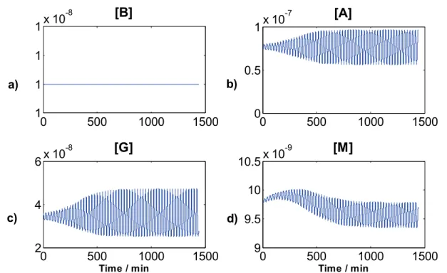
As a first step in numerical analysis of the model, we numerically solved system of ordinary differential equations with rate constants given in Table 1 that satisfies the instability condition (24). The results are given in Figure 1. Oscillatory behavior can be seen, in-volving intermediate species A, M and G, while inter-mediate species B has only non-oscillatory evolution.
Now we were interested to determine the impor-tance of each reaction in the model to the stability of the system. Although only several reactions are in-volved in condition given in equation (24), we cannot exclude other reactions from model without deter-mining their effect on periodic behavior of the system. To do that, we had to use sensitivity analysis. We va-ried rate constants in certain range of values and tested for existence of Andronow–Hopf bifurcation by cal-culating Δ3. Details of this analysis can be found in Ap-pendix I, while the most important results are given in Table 2.
What we have found is that autocatalysis is the dominant process, which is essential for the existence of oscillations in the model, and excluding autocatalysis from the model cancels all negative terms in all dia-gonal minors of matrix V(j), making the system stable. Autoinhibition (R7) on the other hand does not affect 1 2 3 4 5 6 7
4 5 6 7 6 7 4 5 6 7
1 2 3 4 5 6 7 1 2 3 4 5 6 7 3 5 7
4 5 6 7 2 3 4 5 6 7 2 3 4 6
2 2 0 0 0
0 ( ) 2( )
( )
( 2 2 ) 0 2 2 2( )
0 ( ) 2 2
j j j j j j j
j j j j j j j j j j
j
j j j j j j j j j j j j j j j j j
j j j j j j j j j j j j j j
+ + + + + +
+ + + − + + + +
=
− + + + + + + + + + + + + + +
+ + + − + + + + + − + +
stability of the system in general, but this process is necessary for intermediate species M to oscillate. We determined that the rate constants of reactions (R2), (R5), (R7) and (R8) did not have lower limits and re-moving all of them from the model did not affect sys-tem stability. All these reactions, except (R8), are reac-tions that control dynamics of the intermediate species M, and do not interfere in dynamics of other species in system. Although autoinhibition, which is represented by reaction (R7), introduce nonlinear terms in model, these terms did not have a destabilizing effect in our case. Periodic behavior of species M occurs as a result of coupling with intermediate species G, which parti-cipate in autocatalysis.
Table 2. Range of values of rate constants where exists Andronow–Hopf bifurcation
Rate constant
Range
Minimum value Maximum value k1 1.6×10⁻⁸ min–1 2.0×10⁻⁸ min–1 k2 0 7.7×10⁻¹⁰ min–1
k3 1.0×10⁻³ min–1 Inf
k4 4.0×10⁻³ min–1 4.0×10⁻² min–1 k5 0 5.0×10⁻³ min–1 k6 9.7×10¹³ min–1
mol–2 dm6
1.42×10¹⁴ min–1 mol–2 dm6
k7 0 Inf
k8 0 0.65×10⁻² min–1
k9 0.3994 min–1 0.5112 min–1
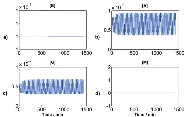
The model is greatly simplified by removing reac-tions (R2), (R5), (R7) and (R8) from it and leaving only reactions that are core of instability responsible for periodic behavior (Table 3). Results of numerical simu-lation of simplified model, very similar to the model known as autocatalator [17] are given in Figure 2. Table 3. Simplified model developed from the model (R1)–(R9)
Reaction Rate constant
1
k
⎯⎯→ B k1 = 1.83×10⁻⁸ min–1 (R1)
B⎯⎯k3→ A k
3 = 1.83 min–1 (R3) A⎯⎯k4→
G k4 = 3.60×10⁻² min–1 (R4) A + 2G⎯⎯k6→ 3G k
6 = 1.26×10¹⁴ min–1 mol–2 dm6 (R6) G⎯⎯k9→
P2 k9 = 0.410 min–1 (R9)
Stoichiometric network analysis of simplified model With the aim to examine the dynamics of the sim-plified model, we performed SNA on it and as a first step we calculated matrix E. New matrix E (Eq. (25)) is reduced to two columns of previous matrix E. All co-lumns that contain removed reactions are cancelled. Both of the remaining extreme currents are essential for the periodic behaviour:
0 500 1000 1500
1 1 1
1x 10
-8
[B]
0 500 1000 1500
0 0.5
1x 10
-7
[A]
0 500 1000 1500
2 4
6x 10
-8
[G]
Time / min
0 500 1000 1500
9 9.5 10
10.5x 10
-9
[M]
Time / min
a) b)
c) d)
Figure 1. Temporal concentration evolution of the species B, A, G and M in the model given in Table 1 obtained by numerically solving system of ordinary differential equations (Eq.(1)) for the intermediates species a) B, b) M, c) A and d) G.
2 3 1 2 3 4 5 6 7 8 9
1 1
0 0
1 1
1 0
0 0
0 1
0 0
0 0
1 1
E E
R R R R R R R R R
=
E (25)
The rates at a steady state, vss, are: ss,1 2 3
v =j +j
(26) ss,3 2 3
v =j +j
ss,4 2
v =j
ss,6 3
v =j
ss,9 2 3
v =j +j
The next step was to examine stability of a steady state by analyzing diagonal minors of matrix V(j):
2 3
2 3 2 3 3
2 3 2 3
0 0 0
0 0 0 0
( )
( ) 0 2
0 0 ( )
j j
j
j j j j j
j j j j
+
=
− + +
− + −
V (27)
This time we found a new instability condition that must be satisfied:
j2 < ј3 (28)
resulting in:
vss,4 < vss,6 (29)
The obtained instability condition is in accordance with the one given in expression (24), since in the re-duced model the rates of reactions (R2) and (R5) are equal to zero.
As we can see from Eq. (27), matrix V(j) for new model can be reduced to 3×3 matrix. This is a result of removing reactions (R2), (R5) and (R7) from the model, because the new model has only 3 intermediate spe-cies. Therefore, the Hurwitz matrix H is also a 3×3 mat-rix, and now for existence of the Andronow-Hopf bifur-cation it is necessary to examine Δ2:
1 3
2 1 23 3
2
0 1
α α
α α α α
Δ = = − =
(30)
This allowed us to obtain the full instability con-dition using the Routh–Hurwitz criterion, which is given in Eq. (24):
A G 4 G A 6
(h +h v) =(h −h v) (31)
We can see from Eq. (31) that for existence of the Andronow–Hopf bifurcation, it must be satisfied that the concentration of intermediate species G must be
0 500 1000 1500
1 1 1
1x 10
-8 [B]
0 500 1000 1500
0 0.5
1x 10
-7 [A]
0 500 1000 1500
0 0.5
1x 10
-7 [G]
Time / min
0 500 1000 1500
-1 0 1 2
[M]
Time / min
b) a)
c) d)
Figure 2. Temporal concentration evolution of the species B, A, G and M in the model given in Table 3 obtained by numerically solving system of ordinary differential equations (Eq.1 with k2 = k5 = k7 = k8 = 0) for the intermediates species a) B, b) M, c) A and d) G.
lower than the concentration of the intermediate spe-cies A, in the steady state. Although the simplified model is enough to simulate the oscillatory evolution of two intermediate species, the other reactions are ob-viously necessary to get results that can be correlated with experimentally obtained evolution of HPA system [18].
CONCLUSION
A systematic approach to the stability analysis of complex chemical reaction networks was applied to a scheme where autocatalytic and autoinhibitory steps are coupled through the same species. The stoichio-metric network analysis was used to find positive and negative feedbacks that may cause concentration oscil-lations of reaction components in the considered mo-del, while sensitivity analysis allowed us to determine the dominant ones.
We have determined that autocatalysis was the dominant process, which was essential for existence of oscillations in the model, while autoinhibition did not play an important role and could be removed from the model without loss of oscillations. This allowed us to simplify the considered model by removing (R2), (R5), (R7) and (R8), and leave only the important reactions. The simplified model is capable to simulate oscillatory evolution, but only of two intermediate species.
We also determined the full instability condition for the reduced model using the Routh–Hurwitz criterion given by Eq. (31). Based on Eq. (31) we can see that for existence of the oscillations in the model concentration of intermediate species G must be lower than the con-centration of the intermediate species A, in the steady state. Therefore, feedback responsible for concentra-tion oscillaconcentra-tions of reacconcentra-tion components is result of in-teraction between intermediate species A and G. Acknowledgement
The present investigations were partially supported by The Ministry of Education, Science and Technolo-gical Development of the Republic of Serbia, under Pro-ject 172015 and 45001.
REFERENCES
[1] Lj. Kolar-Anić, Ž. Čupić, G. Schmitz, S. Anić, Improvement of the stoichiometric network analysis for determination of instability conditions of complex nonlinear reaction systems, Chem. Eng. Sci. 65 (2010) 3718–3728.
[2] S.K. Scott, Reversible Autocatalytic reactions in an iso-thermal CSTR: Multiplicity, stability and relaxation times, Chem. Eng. Sci. 38 (1983) 1701–1708.
[3] P. Gray, S.K. Scott, Autocatalytic reactions in the isother-mal, continuous stirred tank reactor. Isolas and other forms of multistability, Chem. Eng. Sci. 38 (1983) 29–43.
[4] S. Jelić, Ž. Čupić, Lj. Kolar-Anić, Mathematical modeling of the hypothalamic–pituitary–adrenal system activity, Math. Biosci. 197 (2005) 173–187.
[5] B.L. Clarke, Stoichiometric network analysis, Cell Bio-phys. 12 (1988) 237–253.
[6] S. Jelić, Ž. Čupić, Lj. Kolar-Anić, V. Vukojević, Predictive modeling of the hypothalamic-pituitary-adrenal (HPA) function. Dynamic systems theory approach by stoichio-metric network analysis and quenching small Amplitude oscillations, Inter. J. Nonlin. Sci. Num. Sim. 10 (2009) 1451–1472.
[7] B. Clarke, Stability of complex reaction networks, In: I. Prigogine, S. Rice (Eds.), Adv. Chem. Phys., Wiley, New York, 1980, pp. 1–216.
[8] B.L. Clarke, Complete set of steady states for the general stoichiometric dynamical system, J Chem. Phys. 75 (1981) 4970–4979.
[9] B.L. Clarke, Qualitative dynamics and (stability) of che-mical reaction networks, in cheche-mical applications of topology and graph theory, R.B. King (Ed.), Elsevier, Amsterdam, 1983, pp. 322–357.
[10] P.E. Lehner, E. Noma, A new solution to the problem of finding all numerical solutions to ordered metric struc-tures, Psychometrika 45 (1980) 135–137.
[11] R. Schuster, S. Schuster, Refined algorithm and com-puter program for calculating all non-negative fluxes admissible in steady states of biochemical reaction sys-tems with or without some flux rates fixed, Comput. Appl. Biosci. 9 (1993) 79–85.
[12] R. Urbanczik, C. Wagner, An improved algorithm for stoichiometric network analysis: theory and applica-tions, Syst. Biol. 21 (2005) 1203–1210.
[13] J. Gagneur, S. Klamt, Computation of elementary modes: a unifying framework and the new binary ap-proach, BMC Bioinformatics 5 (2004) 175.
[14] Lj. Kolar-Anic, Ž. Čupić, V. Vukojević, S. Anić, Dynamics of Non-linear Processes, Faculty of Physical Chemistry, University of Belgrade, Belgrade, 2011 (in Serbian). [15] B. L. Clarke,W. Jiang, Method for deriving Hopf and
sad-dle-node bifurcation hypersurfaces and application to a model of the Belousov–Zhabotinskii system, J. Chem. Phys. 99 (1993) 4464–4478.
[16] W. Liu, Criterion of Hopf bifurcation without using eigenvalues, J. Math. Anal. App. 182 (1994) 250–256. [17] P. Gray, S. K. Scott, A new model for oscillatory behavior
in closed systems: The Autocatalator, Ber. Bunsenges, Phys. Chem. 90 (1986) 985–996.
[18] V.M. Marković, Ž. Čupić, V. Vukojević, Lj. Kolar-Anić, Predictive modeling of the hypothalamic-pituitary-adre-nal (HPA) axis response to acute and chronic stress, En-docr. J. 58 (2011) 889–904.
[19] J. K. Beers, Numerical methods for chemical engineering - Applications in Matlab, Cambridge University Press, Cambridge, 2007.
APPENDIX I: Sensitivity analysis
The sensitivity analysis we use in this paper is a continuation method where we change values of para-meter of interest ki and determine stability of the sys-tem by calculating the Hurwitz determinant necessary for discussion of oscillatory evolution (in the model considered here Δ3). Change in value of ki causes change in steady state concentrations of intermediate species. Hence, the first step is to calculate steady state concentrations. The steady state concentrations can be calculated from Eq. (4), which can be written in the form:
1 3 d
0 d
b
k k b
t
= − =
(A1.1) 2
2 5 7
d
0 d
m
k k a k mg
t
= + − =
2
3 4 5 6 8
d
0 d
a
k b k a k a k ag k a
t
= − − − − =
2 2
4 6 7 9
d
0 d
g
k a k ag k mg k g
t
= + − − =
Since the relations between current rates and reaction rates can be obtained from the matrix relation:
ss
v =Ej (A1.2)
one simply finds that:
ss,1 1 1 2 3 4 5 26 27
v =k = j +j +j +j +j + j + j
(A1.3) ss,2 2 4 5
v =k =j +j
ss,3 3 1 2 3 4 5 26 27
v =k b=j +j +j +j +j + j + j
ss,4 4 2 4 6
v =k a=j +j +j
ss,5 5 6 7
v =k a=j +j
2
ss,6 6 3 5 7
v =k ag =j +j +j
k 2
ss,7 7 4 5 6 7
v = mg = j +j +j +j
k
ss,8 8 1
v = a= j
k
ss,9 9 2 3
v = g=j +j
Analyzing Eq. (A1.3), we can see that they are corre-lated by the relations:
ss,1 ss,3
v =v
(A1.4) ss,7 ss,2 ss,5
v =v +v
ss,1 ss,4 ss,5 ss,6 ss,8
v =v +v +v +v
ss,3 ss,5 ss,7 ss,8 ss,9
v =v +v +v +v
From these relations we can find analytical solution for steady state concentrations of intermediate species in the following forms:
k k
1 ss
3 =
b
(A1.5)
ss
ss
k k
k
2 5
ss 2
7
a
g
+ =
m
1 2 9 ss 1
ss 2
5 8
4 5 8 6 ss 2
( )
k k k g
k
k k
k k k k g
− −
= =
+
+ + +
a
3 2
6 9 ss 1 2 6 ss 9 4 5 8 ss 1 4 5 2 4 5 8
( ) ( )
[ ( ) ( )] 0
k k g k k k g k k k k g
k k k k k k k
− + − − + + +
+ − − + + =
This method of calculating steady state concen-trations usually cannot be applied to larger models; therefore, it is necessary to use numerical methods for solving system of nonlinear algebraic equation. A nu-merical method that is most often used for this pur-pose is Newton’s method, which is described in Ap-pendix II.
Calculated steady state concentrations are then used for calculating the elements of Jacobian matrix M, which is given in Eq. (10). The next step is to calculate the coefficients of characteristic polynomial αi of mat-rix M. Coefficients αi can be calculated as the sum of all diagonal minors of matrix M with dimensionality i. For example, α1 is equal to the sum of diagonal elements, while α2 is equal to the sum of all diagonal minors of dimension 2, etc. Calculated coefficients of characte-ristic polynomial are used for constructing the Hurwitz matrix H, which in the case of the considered model is a 4×4 matrix given by Eq. (19). From this matrix Δ3 given in Eq. (20), is calculated as a leading principal minor of size 3×3.
APPENDIX II: Newton’s method for solving the system of nonlinear equations
Newton’s method is a root-finding algorithm that uses the first few terms of the Taylor series of a function f(x) in the vicinity of a suspected root. System of nonlinear equations can be given in a form [19,20]:
1 1 2 3 2 1 2 3 3 1 2 3
1 2 3
( , , ... ) 0 ( , , ... ) 0 ( , , ... ) 0
( , , ... ) 0
n n n
n n
f x x x x
f x x x x
f x x x x
f x x x x
=
=
=
=
(A2.1)
For convenience we can think of (x1, x2, x3,…, xn) as a vector x and (f1, f2,…, fn) as a vector-valued function f. With this notation, we can write the system of Eqs. (A2.1) simply as [19]:
( ) 0
f x = (A2.2)
0 0 0 ( ) ( ) ( )( )
f x =f x +J x x−x (A2.3)
where J(x0) is Jacobian of the system at x0. We wish to find x that makes f(x) equal to the zero vectors, so let us choose x1 so that:
0 0 1 0
( ) ( )( ) 0
f x +J x x −x = (A2.4)
Equation (A2.4) can be rewritten as:
0 0
( ) ( )
J x Δ = −x f x (A2.5)
where Δx is (x1–x0). Since J(x0) is a known matrix and
−f(x0) is a known vector, this equation is just a system of linear equations [19,20], which can be solved effi-ciently and accurately. Once we have the solution vec-tor Δx, we can obtain our improved estimate x1 by:
1 0
x =x + Δx (A2.6)
For subsequent steps, we have the following process:
Solve
( )i ( )i
J x Δ = −x f x
Let 1
i i
x+ =x + Δx
For successful application of Newton’s method it is extremely important to have a good initial guess x0 [20]. The best way to get a good initial guess is to start from some known solution x* for some value of para-meter ki0. This solution can be obtained by solving the system of differential equations for ki0. Numerical con-tinuation method is then used to follow the solution as
ki changes its value.
APPENDIX III: Equations of linearized dynamics The stability of the considered steady state is des-cribed with the time evolution of small perturbations of
css, in its vicinity, which will be denoted as Δc [14]. The dynamics close to the steady state can be described by the linearized equation:
ss
d( )
d d
diag( )
d d d
c c
c c
v h c
t t t
+ Δ Δ
= = = ΔS Δ (A3.1)
where: ss
-v v v
Δ = (A3.2)
For small perturbations, the expression SΔv neces-sary for examination of the system evolution in the vicinity of the examined steady state can be linearized by Taylor series taking into account only the first two terms [14]. Let us first do a Taylor expansion for the i-th component:
( ) , ,ss ,ss
ss
( )
j
i i j j q q
q
j q
v
v c c
c
∂
+ − +
∂
Sv = s (A3.3)
By Eq. (4) the first term is equal to zero:
( )i i j j, ,ss 0
j
v =
Sv = s (A3.4)
Now, let us define the relation:
, log log
j i j
i j
i j i
v c v
c v c
∂ ∂
= =
∂ ∂
K (A3.5)
Equation (A3.3) can be transformed into the follow-ing one:
( ) , ,ss ,( ,ss) d
d
i
i i j j q q j q q
j q
c
v h K c c
t
Δ
− =
Sv = s (A3.6)
where hq is reciprocal of the steady state concen-trations of the species q. For all intermediate species Eq. (A3.6) transforms to:
, ,ss , ,ss
d
( )
d
diag( ) diag( )
i j j q q j q q
i j q
T c
v h K c c
t
v h c
Δ
= − =
= Δ
s
S K
(A3.7)
where Jacobian matrix M is defined by: diag( ) diag( )T
v h
=
M S K (A3.8)
Using Eq. (6), Eq. (A3.8) can be transformed to: diag( ) diag( )T
j h
=
IZVOD
NELINEARNI REAKCIONI SISTEM SA AUTOKATALIZOM I AUTOINHIBICIJOM: STABILNOST DINAMIČKIH STANJA Stevan Maćešić1, Željko Čupić2, Ljiljana Kolar-Anić1
1
Univerzitet u Beogradu, Fakultet za fizičku hemiju, Beograd, Srbija
2
Univerzitet u Beogradu, Institut za hemiju, tehnologiju i metalurgiju, Centar za katalizu i hemijsko inžinjerstvo, Beograd, Srbija
(Naučni rad)
Većina realnih sistema su nelinearni, zbog čega je ispitivanje nelinearnih sis-tema od velikog značaja za različite oblasti nauke. Među navedenim sistemima posebno su značajni nelinearni reakcioni sistemi sa povratnom spregom (autoka-taliza i autoinhibicija) za koje su karakteristične pojave kao što su oscilatorna evo-lucija ili haos, i koji se mogu sresti u prirodnim, tehnološkim i ekonomskim siste-mima. Kako se autokataliza i autoinhibicija često istovremeno mogu naći u real-nim sistemima, mi smo analizirali stabilnost jednog reakcionog modela u kome su ova dva procesa spregnuta i pokazali kako stabilnost ovog sistema zavisi od kons-tanti brzina i koncentracija hemijskih vrsta koje su uključene u model. Nelinearni procesi sa povratnom spregom i odgovarajući modeli uglavnom imaju veliki broj promenljivih zbog čega analiza stabilnosti zahteva upotrebu posebnih matematič -kih alata. Za izvođenje analize stabilnosti ispitivanog modela koristili smo
unapre-đeni metod stehiometrijske mrežne analize (SNA) u kombinaciji sa bifurkacionom analizom i analizom osetljivosti. Koristeći navedene metode analize, uspeli smo da izdvojimo reakcije koje predstavljaju jezgro nestabilnosti, i koje su odgovorne za periodičnu evoluciju sistema, na osnovu čega smo uspeli da odredimo uslov koji je neophodan za postojanje Andronov–Hopf bifurkacije.
Ključne reči: Nelinearna dinamika • Ste-hiometrijska mrežna analiza •
![Table 1. Model (R 1 )–(R 9 ) which consists nine reactions [(R 1 )–(R 9 )]](https://thumb-eu.123doks.com/thumbv2/123dok_br/18301349.347711/1.892.463.807.855.1125/table-model-r-r-consists-reactions-r-r.webp)