Ozone zonal asymmetry and planetary waves characterization during Antarctic spring

(1)

ACPD

11, 32337–32361, 2011

Ozone zonal asymmetry over

Antarctica

I. Ialongo et al.

Title Page

Abstract Introduction

Conclusions References

Tables Figures

◭ ◮

Back Close

Full Screen / Esc

Printer-friendly Version Interactive Discussion

Discussion

P

a

per

|

Dis

cussion

P

a

per

|

Discussion

P

a

per

|

Discussio

n

P

a

per

|

Atmos. Chem. Phys. Discuss., 11, 32337–32361, 2011 www.atmos-chem-phys-discuss.net/11/32337/2011/ doi:10.5194/acpd-11-32337-2011

Atmospheric Chemistry and Physics Discussions

This discussion paper is/has been under review for the journal Atmospheric Chemistry and Physics (ACP). Please refer to the corresponding final paper in ACP if available.

Ozone zonal asymmetry and planetary

waves characterization during Antarctic

spring

I. Ialongo, V. Sofieva, N. Kalakoski, J. Tamminen, and E. Kyr ¨ol ¨a

Finnish Meteorological Institute, Earth Observation Unit, Helsinki, Finland

Received: 3 October 2011 – Accepted: 5 December 2011 – Published: 8 December 2011

Correspondence to: I. Ialongo (iolanda.ialongo@fmi.fi)

(2)

ACPD

11, 32337–32361, 2011

Antarctica

I. Ialongo et al.

Title Page

Tables Figures

◭ ◮

Back Close

Full Screen / Esc

Discussion

P

a

per

|

Dis

cussion

P

a

per

|

Discussion

P

a

per

|

Discussio

n

P

a

per

|

Abstract

A large zonal asymmetry of ozone has been observed over Antarctica during winter-spring, when the ozone hole develops. It is caused by a planetary wave-driven dis-placement of the polar vortex. The total ozone data by OMI (Ozone Monitoring In-strument) and ozone profiles by MLS (Microwave Limb Sounder) and GOMOS (Global

5

Ozone Monitoring by Occultation of Stars) were analysed to characterize the ozone zonal asymmetry and the wave activity during Antarctic spring. Both total ozone and profile data have shown a persistent zonal asymmetry over the last years, which is usu-ally observed from September to mid-December. The largest amplitudes of planetary waves at 65◦S (the perturbations can achieve up to 50 % of zonal mean) is observed

10

in October. The wave activity is dominated by the quasi-stationary wave 1 component, while the wave 2 is mainly a travelling wave. Wave numbers 1 and 2 generally explain more than the 90 % of the ozone longitudinal variations. Both GOMOS and MLS ozone profile data showed that ozone zonal asymmetry covers the whole stratosphere and extends up to the altitudes of 60–65 km. The wave amplitudes in ozone mixing ratio

15

decay with altitude, with maxima (up to 50 %) below 30 km. Also the spatio-temporal distributions of the ozone anomaly and the interannual variations were analysed.

The characterization of the ozone zonal asymmetry has become important in the climate research. The inclusion of the polar zonal asymmetry in the climate models is essential for an accurate estimation of the future temperature trends. This information

20

might also be important for retrieval algorithms that rely on ozone a priori information.

1 Introduction

Planetary waves influence the atmospheric circulations and a_ffect the spatial distri-bution and time variations of trace gases in the stratosphere (e.g. Mechoso et al., 1985; Holton et al., 1995). They are generated in the troposphere by thermal and

25

(3)

ACPD

11, 32337–32361, 2011

Antarctica

I. Ialongo et al.

Title Page

Tables Figures

◭ ◮

Back Close

Full Screen / Esc

Discussion

P

a

per

|

Dis

cussion

P

a

per

|

Discussion

P

a

per

|

Discussio

n

P

a

per

|

1984). Stratospheric planetary waves play an important role in shaping the ozone hole (e.g. Solomon, 1999; Fusco and Salby, 1999) through their impact on the polar vortex and on the Brewer-Dobson circulation (BDC). Several studies (e.g. Grytsai et al., 2005, 2007; Crook et al., 2008; Gabriel et al., 2011) have reported a large zonal asymme-try of spring-time ozone over Antarctica. Hio and Yoden (2004) showed that during

5

Antarctic winter-spring the zonal wave number 1 usually gives the main contribution to the ozone zonal asymmetry, while higher zonal wave numbers show travelling struc-tures. The wave-driven displacement of the polar vortex moves low-ozone airmasses equatorwards up to 50◦S. Grytsai et al. (2007) have analysed the total ozone measure-ments by TOMS (Total Ozone Mapping Spectrometer) over Antarctica over the period

10

1979–2005, observing the highest zonal asymmetry (∼60 DU spring average) at 65◦S,

where the edge of the polar vortex is located. The ozone zonal asymmetry over Antarc-tica during spring is caused by the displacement of the ozone hole with respect to the pole because of planetary waves activity. In addition, ozone-rich air accumulates in the South-East sector outside the vortex as a result of the poleward transport of the BDC.

15

The ozone column abundance is related to the tropopause height, which in turn is influenced by the temperature of the lower stratosphere over Antarctica, so that the tropopause raises while the stratosphere cools. Decreased total ozone is associated with lower tropopause pressure (and thus with the higher tropopause), and vice versa. Unlike the influence of tropospheric synoptic processes occurring at midlatitudes, the

20

anti-correlation between total ozone and tropopause height over the Antarctic region has a stratospheric origin (Evtushevsky et al., 2008).

The characterization of the zonal asymmetry has become relevant in the climate re-search, because of its important impact on Southern Hemisphere (SH) climate when a large ozone hole is observed (Crook et al., 2008). Waugh et al. (2009) have

25

(4)

ACPD

11, 32337–32361, 2011

Antarctica

I. Ialongo et al.

Title Page

Tables Figures

◭ ◮

Back Close

Full Screen / Esc

Discussion

P

a

per

|

Dis

cussion

P

a

per

|

Discussion

P

a

per

|

Discussio

n

P

a

per

|

underestimated, too. Also the results achieved by Gillett et al. (2009) suggest that the inclusion of zonal asymmetries in ozone may be essential for the accurate simula-tion of future stratospheric temperature trends. They found a zonal mean temperature response to the ozone zonal asymmetry up to 4 K in the lower stratosphere.

In this paper, the ozone zonal asymmetry during the Antarctic spring over the time

5

period 2005–2010 is characterized by using total ozone observations from the Ozone Monitoring Instrument (OMI) on board the EOS-Aura satellite. This analysis extends the results derived from TOMS data (Grytsai et al., 2007). In addition, the vertical extent of the anomaly is characterized by using ozone profiles measurements by Global Ozone Monitoring by Occultation of Stars (GOMOS) and Microwave Limb Sounder

10

(MLS). The paper is organised as follows. The data are described in Sect. 2. In Sect. 3 the data analysis is explained. The description of the results, including the total ozone zonal asymmetry and the wave activity characterization, is presented in Sect. 4. Summary and discussion conclude the paper.

2 Data

15

2.1 OMI total ozone

The Ozone Monitoring Instrument (OMI) total ozone level 3 data (2005–2010) from the V8 TOMS-like algorithm (Bhartia et al., 2002) were used in this study. OMI is a Dutch-Finnish instrument that flies onboard NASA’s EOS-Aura satellite. The OMI TOMS-like algorithm uses 2 wavelengths (317.5 nm and 331.2 nm under most

con-20

ditions, and 331.2 nm and 360.0 nm for high ozone and high solar zenith angle con-ditions). The longer of the two wavelengths is used to derive the surface reflectiv-ity (or cloud fraction). The shorter wavelength, which is heavily absorbed by ozone, is used to derive total ozone. The OMI total ozone level 3 data are available at http://mirador.gsfc.nasa.gov/ with a spatial resolution of 1◦×1◦. The estimated

root-25

(5)

ACPD

11, 32337–32361, 2011

Antarctica

I. Ialongo et al.

Title Page

Tables Figures

◭ ◮

Back Close

Full Screen / Esc

Discussion

P

a

per

|

Dis

cussion

P

a

per

|

Discussion

P

a

per

|

Discussio

n

P

a

per

|

2.2 GOMOS ozone profiles

GOMOS (http://envisat.esa.int/instruments/gomos) is a stellar occultation instrument, which includes UV-VIS-IR spectrometers for monitoring of ozone and a few other trace gases in the atmosphere (Bertaux et al., 2010). The details of the GOMOS retrieval from night-time UV-VIS measurements are presented in Kyr ¨ol ¨a et al. (2010). The

5

retrieval algorithm relies on the maximum likelihood estimates and uses a minimal amount of a priori information (i.e. it does not use a priori information about the ozone profiles in the Bayesian sense). The retrieval is stabilized by the Tikhonov regulariza-tion (Kyr ¨ol ¨a et al., 2010; Sofieva et al., 2004; Tamminen et al., 2004), which makes the vertical resolution practically independent of angles between the orbital plane and the

10

direction to the star. The vertical resolution (including the smoothing properties of the inversion) of GOMOS ozone profiles is 2 km below 30 km and 3 km above 40 km. From night-time measurements, ozone is retrieved in the altitudes range from∼10 km up to ∼100 km.

The accuracy of the GOMOS retrievals depends on stellar magnitude and spectral

15

class (Tamminen et al., 2010). For this study, dark-limb occultations of hot (e_ff ec-tive temperature≥6000 K) and sufficiently bright (visual magnitude<2) stars were se-lected. The successive occultations of each star are nearly uniformly distributed in the longitudinal direction (maximum 14 occultations per day), and they are carried out ap-proximately at the same local time. GOMOS data coverage is illustrated e.g. in Fig. 1

20

in Sofieva et al. (2009). The precision of individual ozone profiles is 0.5–2 % in the stratosphere and 1–5 % in the mesosphere (Tamminen et al., 2010).

2.3 MLS ozone profiles

The Microwave Limb Sounder (MLS) aboard Aura spacecraft measures thermal mi-crowave limb emission by the atmosphere in five spectral bands from 115 GHz to

25

2.5 THz (Waters et al., 2006). MLS scans the atmosphere from ground to ∼90 km

(6)

ACPD

11, 32337–32361, 2011

Antarctica

I. Ialongo et al.

Title Page

Tables Figures

◭ ◮

Back Close

Full Screen / Esc

Discussion

P

a

per

|

Dis

cussion

P

a

per

|

Discussion

P

a

per

|

Discussio

n

P

a

per

|

each orbit at essentially the same latitudes. Horizontally the profiles are spaced by 1.5◦ great-circle angles along the orbit. The cross-track resolution is defined by the 6 km width of the MLS field of view. The longitudinal separation of MLS measurements is 10◦–20◦ over middle and lower latitudes, which become smaller in the polar regions (Livesey et al., 2011). A typical MLS data coverage in the polar regions is shown e.g. in

5

Fig. 2 of Sofieva et al. (2011). The ozone profiles are retrieved from the spectral region near 240 GHz. For the description of the retrieval algorithm, see Livesey and Snyder (2004).

The vertical resolution of MLS ozone profiles is 2.5–3 km in the stratosphere degrad-ing to 5.5 km in the lower mesosphere. Precisions range from 2–7 % in the

strato-10

sphere to more than 20 % in the mesosphere. Measurements are considered to be valid within the pressure range 316 hPa–0.02 hPa (∼8–75 km). The comparisons of MLS v2.2 ozone profiles show a general agreement at 5–10 % level with stratospheric profiles from satellite, balloon and ground-based data (Froidevaux et al., 2008; Jiang et al., 2007; Livesey et al., 2008). These results are expected to hold also for the v3.3

15

profiles (Livesey et al., 2011), which are used in the current study.

3 Data analysis

The planetary waves signatures in the ozone zonal distribution were investigated using the Fourier series analysis. The ozone longitudinal distribution in a certain latitude band (total ozone and number density or mixing ratio at a certain altitude or pressure)

20

is represented by its Fourier series:

f(λ)=a0

2 +

N

X

m₌1

[a_mcos(mλ)+b_msin(mλ)], (1)

wheref(λ) is the ozone abundance at longitude λ and m is the wave number. The coefficientsa_mandb_mwere obtained fitting the model to the experimental data, by the least squares minimization.

(7)

ACPD

11, 32337–32361, 2011

Antarctica

I. Ialongo et al.

Title Page

Tables Figures

◭ ◮

Back Close

Full Screen / Esc

Discussion

P

a

per

|

Dis

cussion

P

a

per

|

Discussion

P

a

per

|

Discussio

n

P

a

per

|

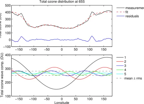
As an example, Fig. 1 shows the results of the harmonic analysis using OMI total ozone data on 16 October 2010. The goodness of the fit was estimated using the coefficient of determination R2, defined as the ratio of the modelled variance to the experimental variance. The analysis ofR2-statistics (applied to the whole data set) has shown that the components with wave numbers from 1 to 3 explain∼95 % of ozone

5

variability. The components with wavenumber higher than 2 are often comparable or below the root mean square (rms) of residuals (in both total ozone and profile mea-surements), thus the retrieved amplitudes of these harmonics cannot be reliable. In the following analyses, only the first two wave numbers are considered.

The wave amplitudes,A_m₌

q

a2_m₊b2_m, averaged over a short time interval (daily for

10

OMI total ozone and 3 days for MLS profiles) include both travelling and stationary wave components. The stationary component of the wave amplitude is isolated by applying the harmonic analysis to the monthly average longitudinal profile.

4 Results

4.1 Total ozone zonal asymmetry

15

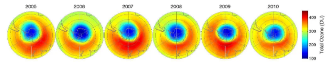
The total ozone zonal asymmetry is caused by the displacement (due to planetary wave activity) of the low ozone polar air (ozone hole) toward the equator and of the mid-latitudinal ozone rich air, which accumulates outside the polar vortex, toward the pole. This is illustrated in Fig. 2 by the mean fields of OMI total ozone over the latitudes 30◦S– 90◦S during October from 2005 to 2010. The polar vortex is generally displaced in the

20

30◦E–30◦W area, while the ozone-rich air is located in the opposite region (150◦E– 200◦E), respect to the South Pole.

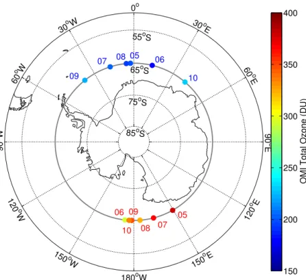
In Fig. 3, the spring (September-October-November average) zonal extremes in OMI total ozone at 65◦S (gray circle) are shown together with their longitudinal position during the period 2005–2010. The di_fferent years are labeled in red for the maxima

25

(8)

ACPD

11, 32337–32361, 2011

Antarctica

I. Ialongo et al.

Title Page

Tables Figures

◭ ◮

Back Close

Full Screen / Esc

Discussion

P

a

per

|

Dis

cussion

P

a

per

|

Discussion

P

a

per

|

Discussio

n

P

a

per

|

During the last 6 yr, the zonal minimum slightly increased (see light blue dots in Fig. 3 for 2009 and 2010 compared to the minima in the previous years), but remained well below the pre-ozone hole values. The zonal minimum at 65◦S slightly moved from

∼0◦ in 2005 to 40◦W in 2009, with a large eastward displacement to ∼40◦E in 2010.

The zonal maximum slightly moved eastward from 150◦E in 2005 to 180◦E in 2010,

5

even though in 2006, when a particularly low ozone maximum (less than 300 DU) was observed (see green point in Fig. 3 labeled with 06), the longitude of the maximum was about 170◦W.

4.2 Wave components in the OMI total ozone zonal distribution

The time evolution from August to December of the daily zonal distribution of the OMI

10

total ozone at 65◦S was compared with the wave components 1 and 2 every year from 2005 to 2010 (Fig. 4). Both wave components show the highest activity during the period from September to November, with visible year-to-year variations. In 2006 and 2008, the wave activity started in mid-September, while it usually begins already in late-August. In 2010, the wave activity has been observed until mid-December with a

15

westward phase change. The time evolution of the wave 1 component shows generally a weakening in early November, before increasing again at the end of the month. This decrease in wave 1 is often compensated by an increase in the wave 2 component.

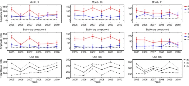
The monthly mean amplitudes of waves 1 and 2 from September to November 2005– 2010 are shown in Fig. 5 (stationary-plus-travelling in the upper panel and stationary

20

in the middle panel). The ozone zonal mean, maximum and minimum values at 65◦S are also shown (Fig. 5, lower panel). The uncertainty on the monthly mean stationary-plus-travelling wave amplitude is obtained from the standard deviation. The error on the stationary wave amplitude is derived from the uncertainty on the fitting coefficients

a_m andb_m, applied to the monthly zonal distribution. Only the wave numbers 1 and 2

25

showed an amplitude larger than the rms of residuals. The wave amplitude is larger in October than in the other months, reaching the value of∼140 DU (∼45 %) in wave

(9)

ACPD

11, 32337–32361, 2011

Antarctica

I. Ialongo et al.

Title Page

Tables Figures

◭ ◮

Back Close

Full Screen / Esc

Discussion

P

a

per

|

Dis

cussion

P

a

per

|

Discussion

P

a

per

|

Discussio

n

P

a

per

|

when the wave 2 amplitude exceeded the wave 1 amplitude by about 20 DU. Wave 1 is mainly a stationary wave, as observed comparing the travelling plus stationary and the stationary only for each month. The other wave numbers are otherwise mostly trav-elling waves; only during November 2009 and 2010 the wave 2 component showed a large stationary component, comparable to wave 1. The wave 1 time yearly-evolution

5

reproduces the mean and the maximum ozone zonal distribution, particularly during September and October, while the minimum values show sometimes a different be-haviour (Fig. 5 – lower panels). This is related to both the position and the shape of the ozone hole and the amount of ozone reaching the polar region. In our analysis sev-eral very high ozone values result in a large zonal mean and increase the difference

10

between maximum and minimum at a given latitude circle.

In September, large wave 1 amplitude values (around 120–130 DU) were observed during 2005 and 2007, while lower values (50–60 DU) in 2006 and from 2008 to 2010; in October the amplitude remained almost stable, ranging from 100 DU to 140 DU and showing anti-correlation with wave 2; in November, the values slightly decreased from

15

80 DU (2005) to 40 DU (2010). The monthly relative amplitudes (not plotted here) show a year-to-year variability similar to the absolute values, with the wave 1 amplitude values ranging from 46 % (October 2009) to 12 % (November 2010).

4.3 Vertical extent of the zonal asymmetry

4.3.1 On the characterization of the ozone anomaly

20

The vertical distribution of ozone and, as a consequence, the vertical extent of the ozone asymmetry is defined not only by planetary waves, but also photochemical pro-cesses that are important at altitudes above∼30 km (e.g. Garcia and Hartmann, 1980).

In the lower stratosphere, ozone can be considered as a passive tracer, thus its dis-tribution is expected to follow the planetary wave perturbation. This means that the

25

(10)

ACPD

11, 32337–32361, 2011

Antarctica

I. Ialongo et al.

Title Page

Tables Figures

◭ ◮

Back Close

Full Screen / Esc

Discussion

P

a

per

|

Dis

cussion

P

a

per

|

Discussion

P

a

per

|

Discussio

n

P

a

per

|

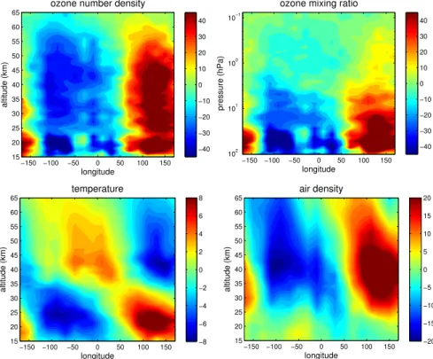
This is illustrated in Fig. 6, which shows deviations from the zonal mean expressed in percent for ozone number density as a function of altitude, ozone mixing ratio as a function of pressure, as well as temperature and density deviations as a function of geometric altitude. These plots are obtained from GOMOS ozone data in September 2003 at 55◦–65◦S and ECMWF air density and temperature data at the locations of

5

GOMOS occultations. (The time period and the latitude band are selected to have the best data coverage and quality.) As seen in Fig. 6, perturbations on ozone number density, which are of nearly constant amplitude up to∼45 km, are in phase with

pertur-bations in air density (and pressure), therefore the analogous perturpertur-bations on mixing ratio decrease more rapidly with decreasing pressure (with increasing altitude). It can

10

be noticed the correlation of ozone and temperature fluctuations below ∼35 km and

anti-correlation above 35–50 km, where chemical processes dominate.

4.3.2 GOMOS observations of wave amplitudes

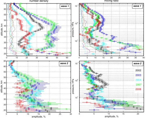
The amplitudes of wave number 1 and 2 detected in GOMOS monthly mean ozone number density and mixing ratio in September (stationary components) are shown in

15

Fig. 7. GOMOS retrievals provide ozone number density as a function of geometric altitude. For representation via mixing ratio at pressure levels, we used ECMWF air density and pressure values at the locations of GOMOS occultations.

The wave amplitudes are significantly larger in number density: they are 20–50 % for wave number 1 and 7–15 % for wave number 2. Wave number 1 is well observed

20

in ozone number density up to 60–65 km altitude, while wave number 2 amplitude ex-ceeds significantly rms of residuals usually below 50–55 km (thus, fitted wave-2 ampli-tudes are not reliable above these altiampli-tudes). In mixing ratio, wave ampliampli-tudes usually are smaller (7–30 % for wave number 1 and 5–10 % for wave number 2), and they decay more rapidly with altitude (decreasing pressure) than in case of ozone number

25

density profiles.

Local minima can be observed in wave amplitude of ozone mixing ratio at altitudes

(11)

ACPD

11, 32337–32361, 2011

Antarctica

I. Ialongo et al.

Title Page

Tables Figures

◭ ◮

Back Close

Full Screen / Esc

Discussion

P

a

per

|

Dis

cussion

P

a

per

|

Discussion

P

a

per

|

Discussio

n

P

a

per

|

as a function of geometric altitude (not shown). The location of these minima corre-sponds to the wave phase transition in temperature, and their appearance is explained by the structure of ozone and air density fields. The amplitudes of wave perturbations vary from year to year. They were especially large, up to 50 % at altitudes 20–50 km, in 2003 and in 2007.

5

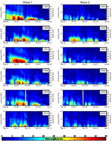
4.3.3 MLS spatio-temporal observations of Antarctic ozone anomaly

Due to a good coverage and temporal resolution, MLS data allow us to study the spatio-temporal evolution of the spring-time Antarctic ozone anomaly. The harmonic analysis described in Sect. 3 has been applied to the MLS mixing ratio data at certain pressure levels, which are used in the MLS inversion algorithm.

10

Figure 8 shows the time series of relative amplitudes of wave 1 and 2 components detected in MLS ozone mixing ratio at 55◦–75◦S in the southern spring seasons of years 2005–2010. These time series have been obtained by applying the harmonic analysis to the three-days running median data, thus they represent perturbations from both travelling and stationary planetary waves. Similarly to GOMOS data (Fig. 7), the

15

wave amplitudes decay with the altitude and up to∼60 km. Maximum amplitudes, being up to 50 %, are observed below 30 km. The wave 1 activity shows many similarities between the years, usually reaching maxima at 20 km towards the end of September and weakening in early November before strengthening again briefly at the end of November. Wave 2 activity is more irregular. It exhibits large short-term variations,

20

in some cases coinciding with weakening wave 1 activity. This feature is observed also in OMI total ozone (Fig. 5). Local minima observed in GOMOS are also visible in MLS data at 35–40 km. Year-to-year variations of planetary wave amplitude are small in September and October, while the November wave activity varies significantly between years.

(12)

ACPD

11, 32337–32361, 2011

Antarctica

I. Ialongo et al.

Title Page

Tables Figures

◭ ◮

Back Close

Full Screen / Esc

Discussion

P

a

per

|

Dis

cussion

P

a

per

|

Discussion

P

a

per

|

Discussio

n

P

a

per

|

5 Summary and discussion

The ozone column data from OMI and ozone profiles from MLS and GOMOS showed a persistent zonal asymmetry over Antarctica during the last 6 southern spring seasons. This was caused by the planetary wave-driven displacement of the polar vortex, which moved the ozone hole to the sector 0◦–40◦W. At the same time, ozone-rich air

occu-5

pied the area outside the vortex, with maximum levels in the sector 150◦–180◦E. The planetary waves were examined by performing Fourier analyses of the ozone fields at a certain latitude or latitude-range. Both the ozone columns and profiles showed similar results. The largest amplitudes of planetary waves (the perturbations can achieve up to 50 %) is observed in October, corresponding to the maximum in the polar vortex jet

10

stream intensity. The wave numbers 1 and 2 generally explain the largest part of the zonal variability. The wave activity is dominated by the quasi-stationary wave 1 com-ponent, while the wave 2 is mainly a travelling wave. Both GOMOS and MLS ozone profile data show that the ozone zonal asymmetry covers the whole stratosphere and extends up to the altitudes of 60–65 km. The wave amplitudes in ozone mixing ratio

15

decay with altitude, with maxima (up to 50 %) below 30 km. The altitude location of the greatest amplitude decreases also with time, because of the effect of the vertical transport in the polar region. Furthermore, the ozone profiles showed that the vertical extent of the ozone asymmetry is related to both the planetary waves activity and the photochemical processes which play an important role above∼30 km. The local

min-20

ima observed in the amplitude profiles correspond to the transition from dynamically to chemically driven regions, and their appearance is explained by the vertical structure of ozone and air density fields.

The spatio-temporal distribution of the ozone anomaly from OMI and MLS (Figs. 4 and 8, respectively) showed similar features, with the maximum wave 1 activity

ob-25

(13)

ACPD

11, 32337–32361, 2011

Antarctica

I. Ialongo et al.

Title Page

Tables Figures

◭ ◮

Back Close

Full Screen / Esc

Discussion

P

a

per

|

Dis

cussion

P

a

per

|

Discussion

P

a

per

|

Discussio

n

P

a

per

|

November 2010 when the wave 2 amplitude exceeded wave 1 by about 20 DU (Fig. 5). The interannual variations in wave amplitudes showed also similar patterns, with the overall largest and smallest wave 1 activity in 2005 and 2010, respectively. In particular, during October 2007 OMI, MLS and GOMOS data showed a large wave 1 amplitude (up to∼40–50 %). Furthermore, the significantly large wave 2 amplitude values (up to

5

45 %) observed by MLS in late October 2005 (Fig. 8, upper-right panel), September– October 2006 (Fig. 8, second row on right column) and early-October 2010 (Fig. 8, lower-right panel), were confirmed by the high values of the wave 2 component showed by OMI (Fig. 4) for the corresponding periods. Some differences in the wave amplitude values, are partly related to the different latitude ranges (65◦S for OMI, 55◦–65◦S for

10

GOMOS and 55◦–75◦S for MLS). These di_fferent zonal bands have been selected in order to ensure the best spatio-temporal resolution for the harmonic analysis. The wave 1 structure showed also an eastward motion (see the slope of the color stripes in Fig. 4) with periods of relative stability for example in November 2006 and during the whole spring 2008. In November 2009 a wave phase change caused a large westward

15

displacement of the minimum/maximum structure.

This spatio-temporal characterization of the ozone zonal asymmetry is relevant for climate research, as it has been observed that the polar zonal asymmetry plays an important role in SH climate when estimating the future temperature trends (e.g. Crook et al., 2008; Waugh et al., 2009; Gillett et al., 2009). This study provides also important

20

information for retrievals algorithms that are based on ozone a-priori information, which usually include only zonal average values.

Acknowledgements. The authors are grateful to the Aura team and the GOMOS team for pro-viding the data. This work was supported by the Academy of Finland (MIDAT and ASTREX projects) and ESA DRAGON-2 programme.

(14)

ACPD

11, 32337–32361, 2011

Antarctica

I. Ialongo et al.

Title Page

Tables Figures

◭ ◮

Back Close

Full Screen / Esc

Discussion

P

a

per

|

Dis

cussion

P

a

per

|

Discussion

P

a

per

|

Discussio

n

P

a

per

|

References

Andrews, D. G., Holton, J. R., and Leovy, C. B.: Middle Atmospheric Dynamics, Academic press, 1987. 32338

Bertaux, J. L., Kyr öl ä, E., Fussen, D., Hauchecorne, A., Dalaudier, F., Sofieva, V., Tamminen, J., Vanhellemont, F., Fanton d’Andon, O., Barrot, G., Mangin, A., Blanot, L., Lebrun, J. C., P érot,

5

K., Fehr, T., Saavedra, L., Leppelmeier, G. W., and Fraisse, R.: Global ozone monitoring by occultation of stars: an overview of GOMOS measurements on ENVISAT, Atmos. Chem. Phys., 10, 12091–12148, doi:10.5194/acp-10-12091-2010, 2010. 32341

Bhartia, P. K. and Wellemeyer, C. W.: TOMS-V8 total O3 algorithm, NASA Goddard Space Flight Center, Greenbelt, MD, OMI Algorithm Theoretical Basis Document Vol II., 2002.

10

32340

Crook, J. A., Gillett, N. P., and Keeley, S. P. E., Sensitivity of Southern Hemisphere climate to zonal asymmetry in ozone, Geophys. Res. Lett., 35, L07806, doi:10.1029/2007GL032698, 2008. 32339, 32349

Evtushevsky, O. M., Grytsai, A. V., Klekociuk, A. R., and Milinevsky, G. P.: Total ozone and

15

tropopause zonal asymmetry during the Antarctic spring, J. Geophys. Res., 113, D00B06, doi:10.1029/2008JD009881, 2008. 32339

Francis, G. and Salby, M.: Radiative influence of Antarctica on the polar night vortex, J. Atmos. Sci, 58, 1300–1309, 2001.

Froidevaux, L., Jiang, Y. B., Lambert, A., Livesey, N. J., Read, W. G., Waters, J. W., Browell,

20

E. V., Hair, J. W., Avery, M. A., McGee, T. J., Twigg, L. W., Sumnicht, G. K., Jucks, K. W., Margitan, J. J., Sen, B., Stachnik, R. A., Toon, G. C., Bernath, P. F., Boone, C. D., Walker,

K. A., Filipiak, M. J., Harwood, R. S., Fuller, R. A., Manney, G. L., Schwartz, M. J., Daffer,

W. H., Drouin, B. J., Cofield, R. E., Cuddy, D. T., Jarnot, R. F., Knosp, B. W., Perun, V. S., Snyder, W. V., Stek, P. C., Thurstans, R. P. and Wagner, P. A.: Validation of Aura Microwave

25

Limb Sounder stratospheric and mesospheric ozone measurements, J. Geophys. Res., 113, D15S20, doi:10.1029/2007JD008771, 2008. 32342

Fusco, A. C. and Salby, M. L.: Interannual variations of total ozone and their relationship to variations of planetary wave activity, J. Clim., 12, 1619–1629, 1999. 32339

Gabriel, A., K ¨ornich, H., Lossow, S., Peters, D. H. W., Urban, J., and Murtagh, D.: Zonal

30

(15)

ACPD

11, 32337–32361, 2011

Antarctica

I. Ialongo et al.

Title Page

Tables Figures

◭ ◮

Back Close

Full Screen / Esc

Discussion

P

a

per

|

Dis

cussion

P

a

per

|

Discussion

P

a

per

|

Discussio

n

P

a

per

|

32339

Garcia, R. and Hartmann, D.: The role of planetary waves in the maintenance of the zonally averaged ozone distribution of the upper stratosphere, J. Atmos. Sci., 37, 2248–2264, 1980. 32345

Gillett, N. P., Scinocca, J. F., Plummer, D. A., and Reader, M. C.: Sensitivity of climate

5

to dynamically-consistent zonal asymmetries in ozone, Geophys. Res. Lett., 36, L10809, doi:10.1029/2009GL037246, 2009. 32340, 32349

Grytsai, A., Grytsai, Z., Evtushevsky, A., Milinevsky, G., and Leonov, N.: Zonal wave numbers

1–5 in planetary waves from the TOMS total ozone at 65◦

S, Ann. Geophys., 23, 1565–1573, doi:10.5194/angeo-23-1565-2005, 2005. 32339

10

Grytsai, A. V., Evtushevsky, O. M., Agapitov, O. V., Klekociuk, A. R., and Milinevsky, G. P.: Struc-ture and long-term change in the zonal asymmetry in Antarctic total ozone during spring, Ann. Geophys., 25, 361–374, doi:10.5194/angeo-25-361-2007, 2007. 32339, 32340

Hartmann, D. L., Mechoso, C. R., and Yamazaki, K.: Observations of wave mean flow interac-tion in Southern Hemisphere, J. Atmos. Sci., 41, 351–362, 1984. 32338

15

Hio, Y. and Yoden, S.: Quasi-periodic variations of the polar vortex in the Southern Hemisphere due to wave-wave interaction, J. Atmos. Sci., 61, 2510–2527, 2004. 32339

Holton, J. R., Haynes, P. H., McIntyre, M. E., Douglass, A. R., Rood, R. B.,

and Pfister, L.: Stratosphere-troposphere exchange, Rev. Geophys., 33, 403–439,

doi:10.1029/95RG02097, 1995. 32338

20

Jiang, Y. B., Froidevaux, L., Lambert, A., Livesey, N. J., Read, W. G., Waters, J. W., Bojkov, B., Leblanc, T., McDermid, I. S., Godin-Beekman, S., Filipiak, M. J., Harwood, R. S., Fuller, R.

A., Daffer, W. H., Drouin, B. J., Cofield, R. E., Cuddy, D. T., Jarnot, R. F., Knosp, B. W., Perun,

V. S., Schwartz, M. J., Snyder, W. V., Stek, P. C., Thurstans, R. P., Wagner, P. A., Allaart, M., Andersen, S. B., Bodeker, G., Calpini, B., Claude, H., Coetzee, G., Davies, J., DeBacker,

25

H., Dier, H., Fujiwara, M., Johnson, B., Kelder, H., Leme, N. P., K ¨onig-Langlo, G., Kyr ¨o, E., Laneve, G., Fook, L. S., Merrill, J., Morris, G., Newchurch, M., Oltmans, S., Parrondos, M. C., Posny, F., Schmidlin, F., Skrivankova, P., Stubi, R., Tarasick, D. W., Thompson, A. M., Thouret, V., Viatte, P., Vomel, H., von der Gathen, P., Yela, M., and Zablocki, G.: Validation of Aura Microwave Limb Sounder Ozone by ozonesonde and lidar measurements, J. Geophys.

30

Res., 112, D24S34, doi:10.1029/2007JD008776, 2007. 32342

(16)

ACPD

11, 32337–32361, 2011

Antarctica

I. Ialongo et al.

Title Page

Tables Figures

◭ ◮

Back Close

Full Screen / Esc

Discussion

P

a

per

|

Dis

cussion

P

a

per

|

Discussion

P

a

per

|

Discussio

n

P

a

per

|

Saavedra de Miguel, L., and Fraisse, R.: Retrieval of atmospheric parameters from GOMOS data, Atmos. Chem. Phys., 10, 11881–11903, doi:10.5194/acp-10-11881-2010, 2010. 32341 Livesey, N. J. and Snyder, W. V.: EOS MLS Retrieval Processes Algorithm Theoretical Basis, Pasadena, California, available at: http://mls.jpl.nasa.gov/data/eosalgorithmatbd.pdf, 2004. 32342

5

Livesey, N. J., Filipiak, M. J., Froidevaux, L., Read, W. G., Lambert, A., Santee, M. L., Jiang,

J. H., Pumphrey, H. C., Waters, J. W., Cofield, R. E., Cuddy, D. T., Daffer, W. H., Drouin, B.

J., Fuller, R. A., Jarnot, R. F., Jiang, Y. B., Knosp, B. W., Li, Q. B., Perun, V. S., Schwartz, M. J., Snyder, W. V., Stek, P. C., Thurstans, R. P., Wagner, P. A., Avery, M., Browell, E. V., Cammas, J. P., Christensen, L. E., Diskin, G. S., Gao, R. S., Jost, H. J., Loewenstein, M.,

10

Lopez, J. D., N ´ed ´elec, P., Osterman, G. B., Sachse, G. W., and Webster, C. R.: Validation of Aura Microwave Limb Sounder O3 and CO observations in the upper troposphere and lower stratosphere, J. Geophys. Res., 113, D15S02, doi:10.1029/2007JD008805, 2008. 32342 Livesey, N. J., Read, W. J., Froidevaux, L., Lambert, A., Manney, G. L., Pumphrey, H. C.,

Santee, M. L., Schwartz, M. J., Wang, S., Cofield, R. E., Cuddy, D. T, Fuller, R. A., Jarnot,

15

R. F., Jiang, J. H., Knosp, B. W., Stek, P. C., Wagner, P. A., and Wu. D. L.: Earth Observing System (EOS) Aura Microwave Limb Sounder (MLS) Version 3.3 Level 2 data quality and description document, JPL D-33509, California Institute of Technology, Pasadena, California, 18 January, 2011. 32342

Mechoso, C. R., Hartmann, D. L., and Farrara, J. D.: Climatology and interannual variability

20

of wave, mean-flow interaction in the southern hemisphere, J. Atmos. Sci., 42, 2189–2206, 1985. 32338

Sofieva, V. F., Tamminen, J., Haario, H., Kyr ¨ol ¨a, E., and Lehtinen, M.: Ozone profile smoothness as a priori information in the inversion of limb measurements, Ann. Geophys., 22, 3411– 3420, doi:10.5194/angeo-22-3411-2004, 2004. 32341

25

Sofieva, V. F., Kyr öl ä, E., Verronen, P. T., Sepp äl ä, A., Tamminen, J., Marsh, D. R., Smith, A. K., Bertaux, J.-L., Hauchecorne, A., Dalaudier, F., Fussen, D., Vanhellemont, F., Fanton d’Andon, O., Barrot, G., Guirlet, M., Fehr, T., and Saavedra, L.: Spatio-temporal observations of the tertiary ozone maximum, Atmos. Chem. Phys., 9, 4439–4445, doi:10.5194/acp-9-4439-2009, 2009. 32341

30

(17)

ACPD

11, 32337–32361, 2011

Antarctica

I. Ialongo et al.

Title Page

Tables Figures

◭ ◮

Back Close

Full Screen / Esc

Discussion

P

a

per

|

Dis

cussion

P

a

per

|

Discussion

P

a

per

|

Discussio

n

P

a

per

|

23317–23348, doi:10.5194/acpd-11-23317-2011, 2011. 32342

Solomon, S.: Stratospheric ozone depletion: a review of concepts and history, Rev. Geophys., 37, 275–316, doi:10.1029/1999RG900008, 1999. 32339

Tamminen, J., Kyr ¨ol ¨a, E., and Sofieva, V. F.: Does prior information improve measurements?, in: Occultations for Probing Atmosphere and Climate – Science from the OPAC-1 Workshop,

5

edited by: Kirchengast, G., Foelsche, U., and Steiner, A. K., 87–98, Springer Verlag, 2004. 32341

Tamminen, J., Kyr ¨ol ¨a, E., Sofieva, V. F., Laine, M., Bertaux, J.-L., Hauchecorne, A., Dalaudier, F., Fussen, D., Vanhellemont, F., Fanton-d’Andon, O., Barrot, G., Mangin, A., Guirlet, M., Blanot, L., Fehr, T., Saavedra de Miguel, L., and Fraisse, R.: GOMOS data characterisation

10

and error estimation, Atmos. Chem. Phys., 10, 9505–9519, doi:10.5194/acp-10-9505-2010, 2010. 32341

Vargin, P. N.: Analysis of an eastward-propagating planetary waves from satellite data on the total ozone content, Izv. RAS. Phy. Atm. Ocean, 39, 327–334, 2003 (in Russian).

Waters, J. W., Froidevaux, L., Harwood, R. S., Jarnot, R. F., Pickett, H. M., Read, W. G., et

15

al.: The Earth Observing System Microwave Limb Sounder (EOS MLS) on the Aura satellite, IEEE T. Geosci. Remote, 44, 1075–1092, doi:10.1109/TGRS.2006.873771, 2006. 32341 Waugh, D. W., Oman, L., Newman, P. A., Stolarski, R. S., Pawson, S., Nielsen, J. E., and

Perl-witz, J.: Effect of zonal asymmetries in stratospheric ozone on simulated Southern

Hemi-sphere climate trends, Geophys. Res. Lett., 36, L18701, doi:10.1029/2009GL040419, 2009.

20

(18)

ACPD

11, 32337–32361, 2011

Antarctica

I. Ialongo et al.

Title Page

Tables Figures

◭ ◮

Back Close

Full Screen / Esc

Discussion

P

a

per

|

Dis

cussion

P

a

per

|

Discussion

P

a

per

|

Discussio

n

P

a

per

|

−150 −100 −50 0 50 100 150

−100 0 100 200 300 400 500

Total ozone (DU)

Total ozone distribution at 65S

measurements fit

residuals

−150 −100 −50 0 50 100 150

100 200 300 400

Longitude

Total ozone wave comp. (DU)

1 2 3 4 5

mean ± rms

Fig. 1. The observed (black solid line - upper panel) distribution from OMI total ozone along

65◦S, compared with the modelled (red dashed line – upper panel) distribution using 1–5 wave

numbers on 16 October 2010. The distribution of the residuals is also shown (blue solid line – upper panel). The spectral components of the wave number 1 to 5 are shown in the lower

(19)

ACPD

11, 32337–32361, 2011

Antarctica

I. Ialongo et al.

Title Page

Tables Figures

◭ ◮

Back Close

Full Screen / Esc

Discussion

P

a

per

|

Dis

cussion

P

a

per

|

Discussion

P

a

per

|

Discussio

n

P

a

per

|

(20)

ACPD

11, 32337–32361, 2011

Antarctica

I. Ialongo et al.

Title Page

Tables Figures

◭ ◮

Back Close

Full Screen / Esc

Discussion

P

a

per

|

Dis

cussion

P

a

per

|

Discussion

P

a

per

|

Discussio

n

P

a

per

|

150

o

W 120

o

W

90

o W 60

oW

30 o_W

0o

30_o E

60

o

E

90

o

E

120 oE

150 o_E

180oW 85o

S 75o

S 65oS

55o S

05 05

06

07 08

09

09 10

07 08 10

OMI Total Ozone (DU)

150 200 250 300 350 400

Fig. 3.OMI total ozone zonal extremes during spring 2005–2010 derived at 65◦

S (this latitude

circle is marked with a gray solid line). The different years are labeled in red for the maxima

(21)

ACPD

11, 32337–32361, 2011

Antarctica

I. Ialongo et al.

Title Page

Tables Figures

◭ ◮

Back Close

Full Screen / Esc

Discussion

P

a

per

|

Dis

cussion

P

a

per

|

Discussion

P

a

per

|

Discussio

n

P

a

per

|

Fig. 4. Time-longitude diagrams of OMI total ozone (first column) at 65◦

S and the related wave components 1 and 2 (second and third column,

respectively) during the period 1 August–31 December from 2005 (top panels) to 2010 (bottom panels). The red and blue colors in the plots of the first column

refer to the maximum and minimum total ozone values, respectively. In the plots of the second and third columns, red colors refer to the maximum positive

(22)

ACPD

11, 32337–32361, 2011

Antarctica

I. Ialongo et al.

Title Page

Tables Figures

◭ ◮

Back Close

Full Screen / Esc

Discussion

P

a

per

|

Dis

cussion

P

a

per

|

Discussion

P

a

per

|

Discussio

n

P

a

per

|

2005 2006 2007 2008 2009 2010

0 50 100 150

Month 9

Amplitude (DU)

2005 2006 2007 2008 2009 2010

0 50 100 150

Stationary component

Amplitude (DU)

2005 2006 2007 2008 2009 2010

200 250 300

OMI TO3

Total Ozone (DU)

Years

2005 2006 2007 2008 2009 2010

0 50 100 150

Month 10

2005 2006 2007 2008 2009 2010

0 50 100 150

2005 2006 2007 2008 2009 2010

200 250 300 350

OMI TO3

Years

2005 2006 2007 2008 2009 2010

0 50 100

Month 11

1 2 res

2005 2006 2007 2008 2009 2010

0 50 100

1 2 res

2005 2006 2007 2008 2009 2010

250 300 350

Years OMI TO3

mean min max

(23)

ACPD

11, 32337–32361, 2011

Antarctica

I. Ialongo et al.

Title Page Abstract Introduction Conclusions References Tables Figures ◭ ◮ ◭ ◮ Back Close

Full Screen / Esc

Printer-friendly Version Interactive Discussion Discussion P a per | Dis cussion P a per | Discussion P a per | Discussio n P a per | longitude altitude (km)

ozone number density

−150 −100 −50 0 50 100 150

15 20 25 30 35 40 45 50 55 60 65 −40 −30 −20 −10 0 10 20 30 40 longitude pressure (hPa)

ozone mixing ratio

−150 −100 −50 0 50 100 150

10−1 100 101 102 −40 −30 −20 −10 0 10 20 30 40 longitude altitude (km) temperature

−150 −100 −50 0 50 100 150

15 20 25 30 35 40 45 50 55 60 65 −8 −6 −4 −2 0 2 4 6 8 longitude altitude (km) air density

−150 −100 −50 0 50 100 150

15 20 25 30 35 40 45 50 55 60 65 −20 −15 −10 −5 0 5 10 15 20

(24)

ACPD

11, 32337–32361, 2011

Antarctica

I. Ialongo et al.

Title Page

Tables Figures

◭ ◮

Back Close

Full Screen / Esc

Discussion

P

a

per

|

Dis

cussion

P

a

per

|

Discussion

P

a

per

|

Discussio

n

P

a

per

|

0 10 20 30 40 50 60

20 25 30 35 40 45 50 55 60 65

number density

altitude, km

0 5 10 15 20 25 30

20 25 30 35 40 45 50 55 60 65

amplitude, %

altitude, km

0 5 10 15 20 25 30 35 40

10−1

100

101

mixing ratio

pressure, hPa

0 5 10 15 20

10−1

100

101

amplitude, %

pressure, hPa

2008

2002

2004 2003

2007

wave 2

wave 1 wave 1

wave 2

Fig. 7. Amplitude (in % of zonal mean) of wave 1 (top panels) and 2 (bottom panels)

com-ponents in September monthly mean ozone profiles at 55◦

–65◦

S in GOMOS ozone number

density (left) and mixing ratio (right). Different years are denoted by different colors (2002 in

(25)

ACPD

11, 32337–32361, 2011

Antarctica

I. Ialongo et al.

Title Page Abstract Introduction Conclusions References Tables Figures ◭ ◮ ◭ ◮ Back Close

Full Screen / Esc

Printer-friendly Version Interactive Discussion Discussion P a per | Dis cussion P a per | Discussion P a per | Discussio n P a per | 20 25 30 35 40 45 altitude (km) pressure (hPa) Wave 1

Sep 05 Oct 05 Nov 05 Dec 05 Jan 06 100 101 102 20 25 30 35 40 45 altitude (km) pressure (hPa) Wave 2

Sep 05 Oct 05 Nov 05 Dec 05 Jan 06 100

101

102

0 5 10 15 20 25 30 35 40 45 50

20 25 30 35 40 45 altitude (km) pressure (hPa)

101

102 20

25 30 35 40 45 altitude (km) pressure (hPa)

101

102

0 5 10 15 20 25 30 35 40 45 50

101

102 20

101

102

0 5 10 15 20 25 30 35 40 45 50

101

102 20

101

102

0 5 10 15 20 25 30 35 40 45 50

101

102 20

101

102

0 5 10 15 20 25 30 35 40 45 50

Sep 10 Oct 10 Nov 10 Dec 10 Jan 11 100 101 102 20 25 30 35 40 45 altitude (km) pressure (hPa)

101

102

0 5 10 15 20 25 30 35 40 45 50

2005 2005

Wave amplitude (%)

2006 2006

Wave amplitude (%)

2007 2007

Wave amplitude (%)

2008 2008

Wave amplitude (%)

2009 2009

Wave amplitude (%)

2010 2010

Wave amplitude (%)

Fig. 8. Time series of amplitudes (in % of zonal mean) of wave 1 and 2 components in MLS

ozone mixing ratio at 55◦–75◦S in September–December, from 2005 (top panels) to 2010