SRef-ID: 1432-0576/ag/2004-22-1487 © European Geosciences Union 2004
Annales
Geophysicae
Multi-resolution analysis of global total ozone column during
1979–1992 Nimbus-7 TOMS period
E. Echer
Instituto Nacional de Pesquisas Espaciais – INPE, POB: 515, 12201-970, S˜ao Jos´e dos Campos, Brazil
Received: 29 July 2003 – Revised: 15 September 2003 – Accepted: 15 October 2003 – Published: 8 April 2004
Abstract.A relatively recent technique, the multi-resolution analysis (MRA), was applied to the global total ozone col-umn measured by the Nimbus-7 TOMS instrument during 1979–1992. Ozone monthly averages were filtered in or-thonormal frequency bands using the Meyer wavelet trans-form, and the ozone variability was analyzed in different time scales: high frequency oscillations (2–4 months), semiannual variation (6 months), annual variation, quasi-biennial oscilla-tion (QBO), El Ni˜no-Southern Oscillaoscilla-tion (ENSO) and solar cycle related variations. MRA was thus showed to be an ef-ficient band-pass filter to isolate different time scale signals. QBO, ENSO and solar cycle related variations in global to-tal ozone are investigated in more detail through spectral and cross-correlation analyses.
Key words. Atmospheric composition and structure (middle atmosphere-composition and chemistry) – General or mis-cellaneous (techniques applicable in three or more fields)
1 Introduction
Total ozone column shows a very well-known global distri-bution, with a minimum of around 260 DU (Dobson Units) at equatorial latitudes, increasing toward poles in both hemi-spheres until a maximum of around 400 DU at sub-polar lat-itudes (Whitten and Prasad, 1985; Stanford et al., 1995). The production of ozone is faster over the equator, where there is more ultraviolet (UV) radiation, than at high lati-tudes and higher elevations. However, the amount of ozone in any region depends on the balance between ozone loss pro-cesses and the transport of ozone by atmospheric motions, as well as on the ozone production. Thus, the high-latitude ozone maximum is a consequence of ozone transport from its source region, the equator, to polar latitudes (Whitten and Prasad, 1985). A strong annual variation is observed in to-tal ozone in both hemispheres, but with opposite phases and a larger amplitude in the Northern Hemisphere. Also, other oscillations are observed, such as the semiannual, the
quasi-Correspondence to:E. Echer (ezequiel@dge.inpe.br)
biennial, quasi-triennial and solar cycle variations (Whitten and Prasad, 1985; Zerefos et al., 1992, 1997; Hood, 1997; Kane et al., 1998).
The quasi-biennial variation in total ozone was first re-ported by Funk and Garnham (1962), as related to the zonal stratospheric wind oscillations of 26–30 months (Reed et al., 1961). This quasi-biennial oscillation (QBO) in strato-spheric winds is a quasi-periodical reversal in zonally sym-metric easterly and westerly wind regimes between 30– 50 hPa (Holton, 1992). It is quantified by a zonal wind in-dex (ZWI), obtained from daily radio soundings at Singa-pore, (104◦E, 1◦N) in pressure levels 100, 70, 50, 30, 20
and 10 hPa (Naujokat, 1986). The phase among total ozone and zonal wind is latitude dependent (Zerefos et al., 1992; Kane et al., 1998). Ozone is in phase with the zonal wind at equatorial regions and has a variation out-of-phase in the extra-tropical latitudes (Zerefos et al., 1992; Hollandsworth et al., 1995; Kane et al., 1998).
The solar cycle signal amplitude on total ozone is around 1–2%, with total ozone reaching maximum values near sunspot maximum (Chandra and Mc Peters, 1994; Zerefos et al., 1997). Direct solar mechanisms for perturbing ozone include changes in solar UV spectral irradiance and changes in the flux of precipitating energetic particles. The solar UV radiation in the 205–250 nm range is responsible for ozone photochemical production, so it is expected that larger in-tensities of UV radiation cause larger ozone photochemical production during solar maximum. Dynamical variations in the lower atmosphere could also be affecting total ozone vari-ability. Hood (1997) analyzed ozone profiles and total ozone with satellite data and inferred that the majority of solar cycle ozone variation occurs in the lower stratosphere, with 85% of variation occurring below 16 hPa. Solar activity in the total ozone column is better seen in the tropics and during peri-ods with no volcanic activity and no synergistic effects from ENSO and QBO (Zerefos et al., 1997). As a measure of so-lar activity one can use the sunspot number or the soso-lar radio flux at 10.7 cm (F10.7), which is the solar output originating in the high solar atmospheric layers of the chromosphere and in lower corona. It has been routinely recorded since Febru-ary 1947. The F10.7does not have significant impacts in the atmosphere, but it is used as a proxy for total and spectral so-lar irradiance, including the ultraviolet irradiance, which is very important in terms of atmospheric processes (Whitten and Prasad, 1985).
In this work global total ozone (65◦S–65◦N) is filtered in
orthonormal frequency levels through multi-resolution anal-ysis (MRA). The characteristic variation of ozone in different time scales is analyzed, and its dependency on quasi-biennial oscillation (QBO), El Ni˜no-Southern Oscillation (ENSO) and solar cycle phenomena are analyzed in detail through multiple-taper spectral and cross-correlation analysis.
2 Data and indices
Global total ozone had been measured by the total ozone mapping spectrometer (TOMS) instrument on board Nimbus-7 from 31 October 1978 to 6 May 1993 (Stanford et al., 1995). In this work data from latitudes higher than 65◦ are not used because of the polar night – TOMS needs the scattered solar light to measure ozone, and data from these latitudes are not available for the whole year (Stolarski et al., 1991). The area coverage is 90% of the globe, but the ozone hole region is not included, which is adequate to study other factors affecting ozone. Total ozone data were obtained from the TOMS homepage, http://jwocky.gsfc.nasa.gov/.
The period during 1979–1992 was chosen for the utiliza-tion of the MRA technique in this work because it is the longest continuous ozone observation period by a unique satellite-borne instrument. The gap in the period around 1995 does not permit the later Earth Probe TOMS data to be used because the wavelet transform used in this work needs continuous time series. Also, the Meteor-3 TOMS data
mea-sured during 1993–1994 were not used because they are from a different instrument, which could introduce bias.
The QBO zonal wind index at 30 hPa (ZWI) is used in this study and it was obtained from Frei Universit¨at Berlin (http://tao.atmos.washington.edu/data sets/qbo/). The SOI used is the one calculated by the method of Ropelewski and Jones (1987), obtained from the Climatic Research Unit, University of East Anglia (ftp://ftp.cru.uea.ac.uk/data). The solar radio flux F10.7 is measured in solar flux units, where one unit equals 10−22Wm−2nm−1. F
10.7 data were ob-tained from the National Geophysical Data Center (http: //www.ngdc.noaa.gov).
3 Multi-resolution analysis
The wavelet transform is a very powerful tool to analyze non-stationary signals and it is used to obtain expansions of a sig-nal using time-localized functions (wavelets) that have good properties of localization in time and in frequency domain (Kumar and Foufola-Georgiou, 1997; Percival and Walden, 2000). The wavelet transform may be continuous or discrete. While continuous wavelet transform calculate coefficients at every possible scale, the discrete wavelet transform chooses scales and positions based on the power of two – the dyadic scales and positions. Thus, the discrete wavelet is a sub-sampling of the continuous one at just the dyadic scales 2j−1, j=1, 2,etc.
The discrete wavelet transform may be used in multi-resolution analysis, which is concerned with the study of signals or process represented at different resolutions and the development an efficient mechanism for going from one resolution to another (Percival and Walden, 2000). Wavelet transform is based on analyzing signals to their components by using a set of basis functions. Wavelet basis functions are related to each other by simple scaling and translation. The original wavelet function, the mother wavelet, is used to gen-erate all basis functions. For the purpose of multi-resolution formulation, there is also a need for a second function, the scaling function, to allow analysis of the function to a finite number of the components (Percival and Walden, 2000).
filtered data (because higher frequencies were split into the D1level and lower frequencies into A2level).
This iterative process could, in theory, continue indefi-nitely. In reality, the decomposition can proceed only until the individual details consist of a single sample or proxy. In practice, the most suitable decomposition of a given signal is selected on an entropy-based criterion or depending on the nature of the signal (Percival and Walden, 2000).
Based on several characteristics of the wavelet functions, it is possible to determine which wavelet is more suitable for a given application. The Meyer wavelet transform is an or-thonormal transform, and it has a scaling function besides the wavelet function, which is necessary for MRA. It is then ad-equate for the goal of decomposing a signal into orthonormal frequency levels.
In this work, the global total ozone series were de-composed until level 6, e.g. S=A6+D1+D2+D3+D4+D5+D6. These levels correspond approximately to the following band-pass filters: D1(2–4 m), D2(4–8 m), D3(8–16 m), D4(16–32 m), D5(32–64 m), D6(64–128 m), and A6(scaling level, long-term variation) frequency levels. ZWI, SOI and F10.7were also decomposed in the same levels, in order to do further analyses. Besides MRA, the multiple taper method (MTM) of spectral analysis (Thomson, 1982) and the cross-correlation analysis were also performed in each wavelet level.
4 Results and discussion
Figure 1 shows the global ozone monthly averages (upper panel, in Dobson Units, DU) and the relative variations in every level for global total ozone, from top to bottom, D1to A6. The global ozone average for this period is 293±6 DU. Global ozone shows a dual peak structure in its annual varia-tion because each hemisphere has maximum in its own spring (Whitten and Prasad, 1985). The long-term negative trend is also seen (Stolarski et al., 1991). The decline is not mono-tonic; a period of rapid decline during the early 1980s is fol-lowed by a period of little change during the late 1980s and by an apparent, more rapid decline in the early 1990s (Hood, 1997). This variation of total ozone could be interpreted as a superposition of a solar cycle variation and a long-term lin-ear and negative trend (Stolarski et al., 1991; Chandra and McPeters, 1994; Hood, 1997; Zerefos et al., 1997). Spec-tral analysis (MTM) was applied to the ozone original data and only the 6 and 12 months were found to be statistically significant at the 95% confidence level.
The D1 level shows high-frequency fluctuations and the period statistically significant at the 95% confidence level is 4 months. In D2level only the semiannual (6 months) fluc-tuation is significant. This semiannual variation is due to the dual peak structure observed in original ozone data (upper panel in Fig. 1), as previously commented.
In the D3 level the only period significant is that of 12 months. The period of 12 months in global ozone appears because the opposite hemispheric annual variations do not
cancel each other, and on a global basis, total ozone has a smaller seasonal variation due to the Northern Hemisphere variation being slightly larger (Heath, 1974; Whitten and Prasad, 1985). The peak of this variation occurs in the first part of year and the minimum in the second part, but the month of peak is not fixed, probably because of the other fluctuations present in this frequency band.
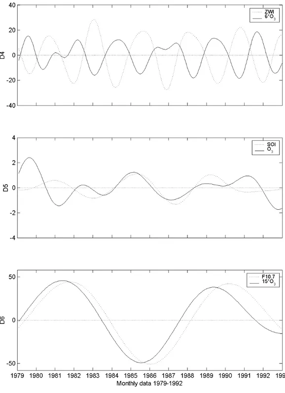
In the D4level the QBO signal is found as significant, 28.0 months (2.3 years), with the oscillations being more irregular than in level D3. In the D5level only a period of 33 months appears, which could or could not be associated with ENSO and the fluctuations are highly irregular. In the D6level the fluctuations are very smooth, with maximum and minimum near solar cycle maximum and minimum, but the 10–11 year solar cycle periods have not been identified, probably be-cause of the short time series used (14 years). Only a period of 84 months (7 years) was found to be statistically signifi-cant. This period is half of the sample size, and it could be a harmonic of the series length. A test with an artificial sinu-soidal series, with a period of 10 years and length of data of 14 years was performed; this periodicity was not identified by MTM. On the other hand, periods of around 6–8 years have been reported in some stations and latitudinal ranges (Kane et al., 1985; 1998; Echer et al., 2001) that could be or not related to solar activity. Another point to consider is that the solar cycle signal could have been split in two levels, D6 (5.3–10.7 years) and A6(periods higher than 10.7 years). A6 level is the scaling level, which is proportional to the aver-age of series (Percival and Walden, 2000). A negative trend can be seen, probably superposed with a long period of si-nusoidal variation. The linear fit to this trend resulted in a correlation coefficient of r2=0.76, but the trend is clearly not linear. Most likely this level has a decrease trend superposed with some longer period oscillations (part of the solar cy-cle variation and other cycy-cles that are not known presently). Meyer wavelet transform was also applied to F10.7, ZWI and SOI data. Figure 2 shows the comparison of the character-istic spectral levels of every phenomenon with total ozone. In the upper panel, D4levels of ozone (continuous line, mul-tiplied by 6 for better visualization) and ZWI at 30 hPa are shown (dotted line). In the middle panel, D5levels for ozone (continuous line) and SOI (dashed line) are presented. And in the lower panel, D6levels for ozone (continuous line mul-tiplied by 15 for better visualization) and F10.7(dotted line) are shown.
The D4 level contains the characteristic period of QBO, 28.0 months. Global ozone and ZWI show the anti-correlated variation, which was also determined from cross-correlation analysis of data. The ZWI variation is very smooth, but with larger amplitudes around 1983–1986. Ozone has in some cycles a variation, that is not very smooth.
Fig. 1.Monthly averages and Meyer wavelet decomposition frequency levels for global total ozone.
ENSO event of 1982–1983, and in period of 1989–1993 the variations are again out-of-phase. Most likely the ozone was mainly affected by ENSO phenomenon during the period 1983–1988 because of ozone reductions caused by ENSO (Zerefos et al., 1992).
The D6 level contains a significant period of around 7 years, both in ozone and F10.7 and it seems to be related to the solar cycle variation. It can be seen that ozone and F10.7, have maximum values during 1981–1982 and 1989–
Fig. 2. Meyer wavelet decomposition frequency levels: D4for zonal wind index and global total ozone (multiplied by 6 for better visual-ization), top panel; D5for SOI and global ozone, middle panel; D6for F10.7and global ozone (multiplied by 15 for better visualization), bottom panel, for the period 1979–1992.
could be mixed with solar signal in these frequency levels because the spacing between the last two big eruptions, El Chichon (1982) and Pinatubo (1991) is similar to the solar cycle period.
Cross-correlations between ozone and every other param-eter have also been calculated. In this work the cross-correlation analysis is performed between parameter 1 and
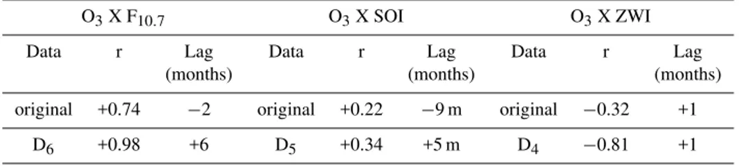
Table 1.Cross-correlation coefficients and lags (in months) between original and decomposed ozone data and ZWI, SOI and F10.7.
O3X F10.7 O3X SOI O3X ZWI
Data r Lag Data r Lag Data r Lag (months) (months) (months)
original +0.74 −2 original +0.22 −9 m original −0.32 +1
D6 +0.98 +6 D5 +0.34 +5 m D4 −0.81 +1
Global ozone data is positively correlated with solar cy-cle, as expected, indicating a variation near in phase (ozone maximum 2 months after F10.7). Ozone is also near in phase with QBO (ozone maximum 1 m before ZWI maximum), but they are anticorrelated. With ENSO, ozone has a lower cor-relation and a lag of−9 months (ozone maximum 9 months after SOI).
It is seen that the frequency levels cross-correlation coef-ficients are higher than the original data coefcoef-ficients. The coefficients increase from around 0.50 to 0.98 for ozone and solar cycle F10.7index correlation, and from−0.30 to−0.80 for ozone and QBO (ZWI) correlation. These results indi-cate that both solar and QBO components in ozone were ad-equately isolated by the MRA filtering. On the other hand, the correlation between ozone and ENSO was not greatly im-proved (from around 0.2 to 0.3) most likely due to the irreg-ular character of ENSO, which does not have strong period-icities as solar and QBO phenomena, but it encompasses a broad range of periods, behaving irregularly (Enfield, 1989). There is also the possibility that part of the ENSO signal was split in the D6level, especially for periods higher than 5 years.
Several works have analyzed the correlations between ozone and other parameters using filtered data. Zerefos et al. (2001), who used Dobson data during 1964–1994, have found for the latitude range 0◦–60◦N a correlation coefficient r=0.45 between ozone and F10.7. Chandra (1991) have used TOMS data for 40◦S–40◦N and after filtering for annual-QBO variations, have found r=0.61 for ozone and F10.7, with variations in phase. Zerefos et al. (1997) have found that the statistical correlation between ozone and F10.7outside the latitude range 40◦S–40◦N is low and not statistically signif-icant, probably because it is masked by much higher ozone variability at these higher latitudes. They have found a corre-lation of around r=0.40 for the range 0◦–30◦S. The
correla-tion coefficient for global ozone and F10.7filtered data found in this work is r=0.98, indicating that the wavelet filtering had obtained a good performance on isolating the solar signal on ozone.
The correlation with QBO resulted, in the wavelet filtered D4level, in a lag of 1 m and r=−0.81. This result is global and it can differ greatly from latitude to latitude, as it was shown by Kane et al. (1998).
5 Conclusions
Multi-resolution analysis (MRA) was applied to the global total ozone series recorded by the Nimbus-7 TOMS instru-ment during 1979–1992. Ozone monthly average data were decomposed in orthonormal frequency levels through the Meyer wavelet transform. The MRA proved to be a very efficient band-pass filtering technique, with high-frequency terms, semi-annual, annual, QBO, ENSO and solar cycle related variations in isolated ozone. Semiannual, annual and annual periodicities were found by spectral analysis in each frequency band. Correlation between ozone and QBO (ZWI) and between ozone and solar (F10.7)activity was ob-served to be much higher in their respective frequency bands than in the original data. However, the correlation between ozone and ENSO (SOI) was not observed to improve in fil-tered data, probably because of the irregular characteristic of ENSO/SOI series. It may be concluded that MRA can be an efficient band-pass filtering technique that can be used for several geophysical studies.
Acknowledgements. Thanks to TOMS processing team for ozone
data, to NGDC, Frei Universit¨at Berlin and Climatic Research Unit-University of East Anglia, for F10.7, ZWI and SOI data, respec-tively.
Topical Editor O. Boucher thanks C. Zerefos and another referee for their help in evaluating this paper.
References
Bojkov, R. D.: The 1983 and 1985 anomalies in ozone distribution in perspective, Mon. Weather Review, 115, 2187–2201, 1987. Chandra, S.: The solar UV related change in total ozone from a
solar rotation to a solar cycle, Geophys. Res. Lett., 18, 837–841, 1991.
Chandra, S. and McPeters, R. D.: The solar cycle variation of ozone in the stratosphere inferred from Nimbus-7 and NOAA-11 satel-lites, J. Geophys. Res., 99, 20 665–20 671, 1994.
Echer, E., Kirchhoff, V. W. J. H., Sahai, Y., and Paes Leme, N.: A study of the solar cycle signal on total ozone over low-latitude Brazilian observation stations, Adv. Spa. Res., 27, 1983–1986, 2001.
Enfield, D. B.: El Ni˜no, Past and Present, Rev. Geophys., 27, 159– 187, 1989.
Hasebe, F.: A global analysis of the fluctuation of total ozone. II Non-stationary annual oscillation, quasi-biennial oscillation and long-term variation in total ozone, J. Meteorol. Soc. Jpn, 58, 104–110, 1980.
Heath, D. F.: Recent advances in satellite observations of solar vari-ability and global atmospheric ozone, NASA Preprint X 912 74 190, GSFC, 1974.
Hollandsworth, S. M., Bowman, K. P., and McPeters, R. D.: Obser-vational study of the quasi-biennial oscillation in ozone, J. Geo-phys. Res., 100, 7347–7361, 1995.
Holton, J. R.: An introduction to Dynamic Meteorology, Academic Press, San Diego, USA, 511 p., 1992.
Hood, L. L.: The solar cycle variation of total ozone: Dynamical forcing in the lower stratosphere, J. Geophys. Res., 102, 1355– 1370, 1997.
Kane, R. P., Sahai, Y., and Teixeira, N. R.: Maximum Entropy Spec-tral Analysis of Total Ozone, PAGEOPH, 122, 747–762, 1985. Kane, R. P., Sahai, Y., and Casiccia, C.: Latitude dependence of the
quasi-biennial oscillation and quasi-triennial oscillation charac-teristics of total ozone measured by TOMS, J. Geophys. Res., 103, 8477–8490, 1998.
Kumar, P. and Foufoula-Georgiou, E.: Wavelet Analysis for geo-physical applications, Rev. Geophys., 35, 385–412, 1997. Naujokat, B.: An update of the observed quasi-biennial oscillation
of the stratospheric winds over the tropics, J. Atmos. Sci., 17, 1873–1877, 1986.
Percival, D. B. and Walden, A. T.: Wavelet Methods for Time Series Analysis, Cambridge University Press, 2000.
Reed, R. J., Campbell, W. J., Rasmussen, L. A. and Rogers, D. J.: Evidence of a downward propagating annual wind reversal in the equatorial stratosphere, J. Geophys. Res., 66, 813–820, 1961. Ropelewski, C. F. and Jones, P. D.: An extension of the
Tahiti-Darwin Southern Oscillation Index, Monthly weather Review, 115, 2161–2165, 1987.
Stanford, J. L., Ziemke, J. R., McPeters, R. D., Krueger, A. J., and Bhartia, P. K.: Spectral Analyses, Climatology and Interannual Variabilitiy of Nimbus-7 TOMS Version 6 Total Column Ozone, NASA Reference Publication 1360, NASA Scientific and Tech-nical Information Branch, 1995.
Stolarski, R. S., Bloomfield, P., McPeters, R. D.: Total ozone trends deduced from Nimbus-7 TOMS data, Geophys. Res. Lett., 18, 1015–1018, 1991.
Thomson, D. J.: Spectrum estimation and harmonic analysis, Proc. IEEE, 70, 1055–1096, 1982.
Whitten, R. C. and Prasad, S. S.: Ozone in Free Atmosphere, Van Nostrand Reinhold Company, New York, 288, 1985.
Zerefos, C. S., Bais, A. F., Ziomas, J. C., and Bojkov, R. D.: On the relative importance of Quasi-Biennial Oscillation and El Ni˜no/Southern Oscillation in the Revised Dobson Total Ozone Records, J. Geophys. Res., 97, 10 135–10 144, 1992.
Zerefos, C. S., Tourpali, K., Bojkov, B. R., Balis, D. S., Rognerund, B., and Isaksen, I. S. A.: Solar activity-total column ozone re-lationships: Observations and model studies with heterogeneous chemistry, J. Geophys. Res., 102, 1561–1569, 1997.