Drivers of changes in stratospheric and tropospheric ozone between
year 2000 and 2100
Antara Banerjee1,a, Amanda C. Maycock1,2,b, Alexander T. Archibald1,2, N. Luke Abraham1,2, Paul Telford1,2, Peter Braesicke1,2,c, and John A. Pyle1,2
1Department of Chemistry, University of Cambridge, Cambridge, UK
2NCAS-Climate, Department of Chemistry, University of Cambridge, Cambridge, UK
anow at: Department of Applied Physics and Applied Mathematics, Columbia University, New York, NY, USA bnow at: School of Earth and Environment, University of Leeds, Leeds, UK
cnow at: Karlsruhe Institute of Technology, Institute for Meteorology and Climate Research, Karlsruhe, Germany Correspondence to:Antara Banerjee ([email protected])
Received: 22 September 2015 – Published in Atmos. Chem. Phys. Discuss.: 5 November 2015 Revised: 9 February 2016 – Accepted: 13 February 2016 – Published: 4 March 2016
Abstract.A stratosphere-resolving configuration of the Met Office’s Unified Model (UM) with the United Kingdom Chemistry and Aerosols (UKCA) scheme is used to inves-tigate the atmospheric response to changes in (a) greenhouse gases and climate, (b) ozone-depleting substances (ODSs) and (c) non-methane ozone precursor emissions. A suite of time-slice experiments show the separate, as well as pair-wise, impacts of these perturbations between the years 2000 and 2100. Sensitivity to uncertainties in future greenhouse gases and aerosols is explored through the use of the Repre-sentative Concentration Pathway (RCP) 4.5 and 8.5 scenar-ios.
The results highlight an important role for the stratosphere in determining the annual mean tropospheric ozone response, primarily through stratosphere–troposphere exchange (STE) of ozone. Under both climate change and reductions in ODSs, increases in STE offset decreases in net chemical pro-duction and act to increase the tropospheric ozone burden. This opposes the effects of projected decreases in ozone pre-cursors through measures to improve air quality, which act to reduce the ozone burden.
The global tropospheric lifetime of ozone (τO3) does not change significantly under climate change at RCP4.5, but it decreases at RCP8.5. This opposes the increases inτO3 sim-ulated under reductions in ODSs and ozone precursor emis-sions.
The additivity of the changes in ozone is examined by comparing the sum of the responses in the single-forcing
ex-periments to those from equivalent combined-forcing exper-iments. Whilst the ozone responses to most forcing combi-nations are found to be approximately additive, non-additive changes are found in both the stratosphere and troposphere when a large climate forcing (RCP8.5) is combined with the effects of ODSs.
1 Introduction
al., 2014). The magnitudes of natural emission sources of tro-pospheric ozone precursors are also likely to be affected by future changes in climate and land use (Squire et al., 2014) through changes in, for example, wildfire activity (Yue et al., 2013), lightning activity (Grewe, 2009; Banerjee et al., 2014) and the amount of isoprene emitted from vegetation (Sander-son, 2003; Pacifico et al., 2009).
The latest Intergovernmental Panel on Climate Change (IPCC) report adopted representative concentration pathway (RCP) scenarios for future emissions of greenhouse gases and aerosols, which are labelled according to the total ra-diative forcing at the year 2100 relative to the preindustrial (RCP2.6, 4.5, 6.0 and 8.5). Future ODS emissions are equiv-alent for RCP4.5, 6.0 and 8.5 (Meinshausen et al., 2011). All RCPs share the assumption of stringent future air quality legislation, and include strong reductions in non-methane an-thropogenic emissions. Projections of methane concentration vary greatly between the RCPs. RCP2.6, 4.5 and 6.0 assume different trajectories for methane, but all project a decrease by 2100 as compared to 2000 (van Vuuren et al., 2011). In contrast, RCP8.5 projects more than a doubling in methane over this period.
In the troposphere, the numerical budget of ozone is widely used as a metric to gain insight into processes con-trolling ozone amounts. In practice, many studies calcu-late the budget of odd oxygen (Ox) to account for species
that rapidly interconvert with ozone. In this study, Ox is
defined as the sum of ozone, O(3P), O(1D), NO2, 2NO3,
3N2O5, HNO3, HNO4, peroxyacetyl nitrate (PAN),
perox-ypropionyl nitrate (PPAN) and peroxymethacrylic nitric an-hydride (MPAN). Although the exact definition varies be-tween studies, in any case, ozone represents the majority of Ox. The budget consists of four terms: chemical production
(P(Ox)), chemical loss (L(Ox)), deposition to the surface
(D(Ox)) and stratosphere–troposphere exchange (STE). The
two chemical terms may be combined to give the net chem-ical production (NCP=P(Ox) minusL(Ox)). STE is
com-monly inferred as the net transport of ozone from the strato-sphere to the tropostrato-sphere required to close the tropospheric budget; this is the definition employed throughout the re-mainder of this study, unless otherwise stated. The processes that determine tropospheric ozone are strongly buffered. As a result, the inter-model spread in estimates of the contempo-rary ozone burden (e.g. for the year 2000) is small compared to the spread in other terms of the budget, as evident from several multi-model comparisons (IPCC, 2001; Stevenson et al., 2006; Wild, 2007; Young et al., 2013).
There exists a large body of literature that assesses the im-pact of future climate change on tropospheric ozone, includ-ing the multi-model studies mentioned above. Several fea-tures are robust across models: increased tropospheric ozone destruction through increased water vapour abundances (e.g. Johnson et al., 1999), which, for most models, leads to a de-crease in NCP, and an inde-crease in STE due to a strengthened
Brewer–Dobson circulation (BDC) (e.g. Collins et al., 2003; Sudo et al., 2003; Zeng and Pyle, 2003).
On the other hand, isolating the impacts of declining ODS concentrations, and the associated recovery of stratospheric ozone, on tropospheric composition has received attention in only a few studies (Kawase et al., 2011; Morgenstern et al., 2013; Zhang et al., 2014). Effects could occur through two main mechanisms: (i) increases in STE and (ii) increases in overhead ozone column with concomitant reductions in tro-pospheric photolysis rates. In such ODS-only scenarios, the aforementioned studies have shown the increase in STE to be the dominant influence on the tropospheric ozone burden, while changes in photolysis rates drive a reduction in tro-pospheric concentrations of the hydroxyl radical (OH) and increase the methane lifetime.
This study employs the Met Office’s Unified Model con-taining the United Kingdom Chemistry and Aerosols sub-model (UM-UKCA) in a process-based approach to separate the impacts of future changes in climate, ODSs and emis-sions of non-methane ozone precursors on ozone. The anal-ysis focuses on changes between 2000 and 2100 under the RCP4.5 and 8.5 climate forcing scenarios. Note that future methane emissions are highly uncertain and changes in its abundance, particularly at RCP8.5, will likely have large tro-pospheric and stratospheric impacts (Randeniya et al., 2002; Fleming et al., 2011; Revell et al., 2012, 2015; Young et al., 2013) that are not the focus of this study. Instead, we wish to isolate other drivers of ozone changes, in particular, the role of a change in mean climate state at RCP8.5, without the as-sumption of a large increase in methane abundance. Hence, the methane boundary condition is kept fixed in all sensitiv-ity tests, although its radiative forcing effect is included in future changes to climate.
Mechanisms for stratosphere–troposphere coupling are highlighted through changes in stratospheric circulation and in chemistry. We do not discuss the detailed mechanisms that underlie changes in the global circulation (e.g. McLandress and Shepherd, 2009; Butchart et al., 2010; Hardiman et al., 2013). Particular focus is rather placed on assessing impacts on the global burden of tropospheric ozone. To this end, the global, tropospheric Ox budget is analysed in detail. To the
best of our knowledge, few other studies have diagnosed this budget for the RCP scenarios (Kawase et al., 2011), which, as discussed by Young et al. (2013), was a shortcoming of the recent Atmospheric Chemistry and Climate Model Inter-comparison Project (ACCMIP).
periments are presented in two sections. Section 3 focuses on changes in temperature and stratospheric ozone. Section 4 then discusses tropospheric ozone and how, in particular, it is influenced by stratospheric effects. Concluding remarks are given in Sect. 5.
2 Methodology
2.1 Model description and experimental setup
This study uses an atmosphere-only, stratosphere-resolving configuration of UM-UKCA at a resolution of N48L60 (3.75◦×2.5◦, with 60 hybrid-height levels extending up to 84 km). A detailed description of the model can be found in Banerjee et al. (2014). Briefly, the model combines the pre-viously validated UKCA stratospheric (Morgenstern et al., 2009) and tropospheric (O’Connor et al., 2014) chemical schemes. These include stratospheric gas-phase ozone chem-istry; heterogeneous reactions on polar stratospheric clouds (PSCs); and oxidation of methane, carbon monoxide (CO) and non-methane volatile organic compounds (NMVOCs). Natural forcings (volcanic eruptions, solar cycle variations) are not included in the experiments, but the model does in-ternally generate the quasi-biennial oscillation (QBO). Emis-sions of NOxfrom lightning (LNOx) are parameterised as a
function of cloud-top height (Price and Rind, 1992, 1994) and thus can vary with changes in convection (Banerjee et al., 2014). Ozone and water vapour are interactive between the chemistry and radiation schemes.
We present results from a series of time-slice experi-ments, forced with fixed seasonally varying boundary con-ditions. These include time-averaged sea surface tempera-tures (SSTs) and sea ice, a uniform fixed CO2
concentra-tion, uniform surface mixing ratios for other greenhouse gases (GHGs) and ODSs, and emissions of NOx, CO and
NMVOCs. Each simulation is integrated for 20 years, with the last 10 years used for analysis.
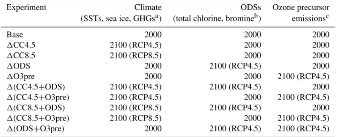
A control simulation (Base) is forced by full year 2000 conditions; the remaining experiments perturb one or more of the boundary conditions to year 2100 levels. The experi-ments are detailed in Table 1, which has been updated from Banerjee et al. (2014). The three types of perturbation de-tailed in that paper, and briefly described now, are as follows: i. Climate change (1CC) – the climate is changed by varying SSTs, sea ice and GHG concentrations (CO2,
CH4, N2O, CFCs and HCFCs) in the radiation scheme
only. Perturbations to year 2100 levels follow two RCP scenarios – RCP4.5 and RCP8.5 (van Vuuren et al., 2011) – with climatological SSTs and sea ice obtained from simulations of the HadGEM2-CC
exist some, but not large, differences in ODS concen-trations between RCP scenarios, and thus RCP4.5 is arbitrarily adopted. Note that the abundance of ODSs at 2100 is still larger than that at 1960. The change in ODSs is applied to the chemistry scheme only and is uncoupled from the radiation scheme.
iii. Ozone precursor emissions (1O3pre) – a reduction in NOx, CO and NMVOC emissions from anthropogenic
and biomass burning sources is considered. The RCP4.5 scenario is also followed here, although this is some-what arbitrary since all RCP scenarios project ag-gressive mitigations of these emissions, and there are not large differences between them (Lamarque et al., 2013). Methane and natural emissions (including iso-prene emissions) remain unchanged.
We emphasise that methane remains at year 2000 levels within the chemistry scheme in all experiments, although, as mentioned, its radiative impact is included in the effects of future climate change.
2.2 Stratospheric ozone tracer
To isolate the influence of the stratosphere on the tropo-sphere through STE, we implement a “stratospheric ozone” tracer, O3S, into the model in a manner similar to Collins
et al. (2003). In the stratosphere, defined as altitudes above the thermal tropopause (WMO, 1957), O3S is constrained to
equal ozone at every model time step. In the troposphere, O3S evolves freely. Following Roelofs and Lelieveld (1997),
O3S has no tropospheric chemical production (unlike
tro-pospheric ozone, which is formed from NO2 photolysis);
however, we do consider its loss through O(1D)+H 2O,
HO2+O3, OH+O3 and dry deposition. Loss of O3S
through reactions which conserve Ox is not considered. In
this way, ozone that originates in the stratosphere can be traced through the troposphere.
The O3S tracer was implemented in the following
exper-iments: Base, 1CC8.5, 1ODS and 1(CC8.5+ODS), us-ing the model-simulated, time-varyus-ing thermal tropopause height and ozone field of each run. The impact of the choice of tropopause definition on O3S has not been investigated;
Lin et al. (2012) find in their CCM that seasonally averaged surface O3S abundances are 5–8 ppbv higher when defined
by the thermal tropopause compared to the “e90 tropopause”, which essentially differentiates tropospheric from strato-spheric air based on mixing timescales (Prather et al., 2011). However, although there are quantitative differences in ab-solute O3S abundances between different tropopause
Table 1.List of model simulations.
Experiment Climate ODSs Ozone precursor
(SSTs, sea ice, GHGsa) (total chlorine, bromineb) emissionsc
Base 2000 2000 2000
1CC4.5 2100 (RCP4.5) 2000 2000
1CC8.5 2100 (RCP8.5) 2000 2000
1ODS 2000 2100 (RCP4.5) 2000
1O3pre 2000 2000 2100 (RCP4.5)
1(CC4.5+ODS) 2100 (RCP4.5) 2100 (RCP4.5) 2000
1(CC4.5+O3pre) 2100 (RCP4.5) 2000 2100 (RCP4.5)
1(CC8.5+ODS) 2100 (RCP8.5) 2100 (RCP4.5) 2000
1(CC8.5+O3pre) 2100 (RCP8.5) 2000 2100 (RCP4.5)
1(ODS+O3pre) 2000 2100 (RCP4.5) 2100 (RCP4.5)
aChanges in GHGs are imposed within the radiation scheme only.
bRelative to Base, runs containing1ODS include total chlorine and bromine reductions at the surface of 2.3 ppbv (67 %) and 9.7 pptv (45 %), respectively.
cRelative to Base, runs containing1O3pre include average global and annual emission changes of NO (−51 %), CO (−51 %), HCHO (−26 %), C2H6(−49 %), C3H8(−40 %), CH3COCH3(−2 %), and CH3CHO (−28 %).
3 Stratospheric ozone
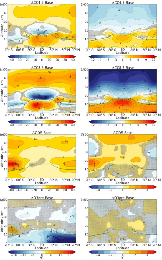
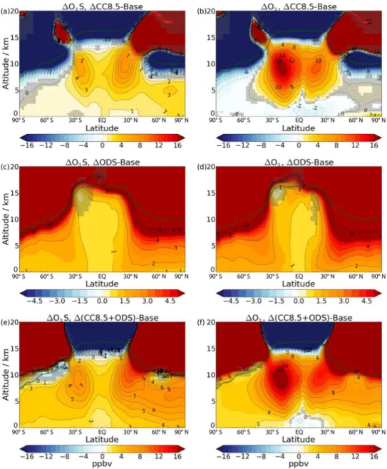
Figure 1 shows changes in zonal and annual mean ozone and temperature compared to the Base run for experiments in which a single type of perturbation has been imposed in turn. Figure 2 shows changes in stratospheric and tropo-spheric column ozone over the tropics for the single- and combined-forcing experiments. The tropics are highlighted as a region of particular interest, since it is here that total column ozone is not expected to recover to pre-1980 val-ues this century (Austin et al., 2010; WMO, 2011; Eyring et al., 2013). Although some discussion of tropospheric ozone is given, the following subsections focus mainly on strato-spheric changes. Whilst many of these results have, at least qualitatively, been established in other studies, the aim is to highlight those changes in the large-scale stratospheric state which bear some relevance for tropospheric ozone, which is discussed in Sect. 4.
3.1 Climate change under RCP4.5 and 8.5
Experiments 1CC4.5 and1CC8.5 show a pattern of tem-perature response (Fig. 1b and d) that is robust across cli-mate models (IPCC, 2013). The troposphere warms across the globe, with a maximum change in excess of 3/9 K (1CC4.5/1CC8.5) in the tropical upper troposphere; the stratosphere cools, primarily due to increased longwave emission by CO2(Fels et al., 1980). In the middle and upper
stratosphere, where Ox(i.e. O+O3here) is in photochemical
steady state, it is well established that cooling slows down the rate of catalytic Oxdestroying cycles (Haigh and Pyle, 1982;
Jonsson et al., 2004). This effect leads to ozone increases in this region (Fig. 1a and c), which partly mitigate the CO2
-induced cooling through increased absorption of shortwave radiation. The magnitude of this effect has been quantified using simulations (not otherwise discussed) performed
un-der1CC4.5/1CC8.5 forcings, but in which a fixed, time-varying 3-D ozone climatology from the Base run is em-ployed in the calculation of radiative heating rates. These simulations show the radiative offset of ozone changes to reach 2/4 K (1CC4.5/1CC8.5) at 40 km.
In the tropical lower stratosphere, where photochemical lifetimes are long and ozone is predominantly under dynam-ical control, a decrease in ozone arises from enhanced up-welling of ozone-poor air from the troposphere, which is as-sociated with a strengthened BDC (e.g. SPARC CCMVal, 2010; WMO, 2011; IPCC, 2013). This localised decrease in ozone is enhanced by the greater overlying ozone column, which reduces chemical production due to the “reversed self-healing” effect (Haigh and Pyle, 1982; Meul et al., 2014), but this is partly mitigated by increases in lightning-derived ozone/NOx due to deeper convection in a warmer climate
(Banerjee et al., 2014).
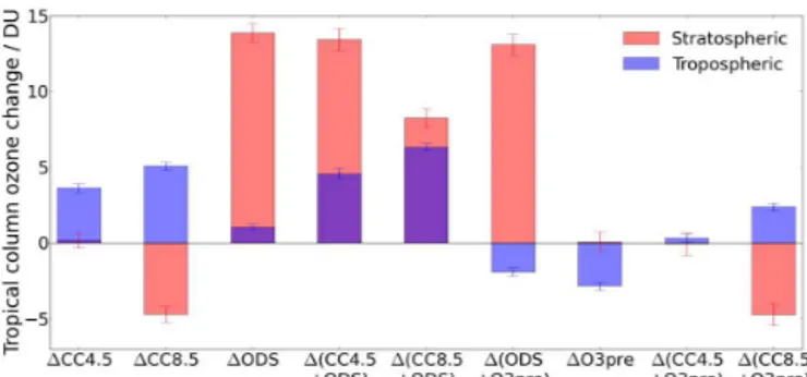
For the tropical stratospheric ozone column, Fig. 2 il-lustrates a very small and statistically insignificant increase of 0.2 DU (0.1 %) in 1CC4.5 but a decrease of 4.7 DU (2 %) in1CC8.5. Thus, the opposite-signed ozone changes in the lower and upper tropical stratosphere do not scale similarly with climate forcing in their contribution to the partial column. Whilst there is a near cancellation be-tween these effects in1CC4.5, the stronger BDC dominates in1CC8.5. These results are qualitatively consistent with those from transient Coupled Model Intercomparison Project Phase 5 (CMIP5) simulations using chemistry–climate mod-els (CCMs) (Eyring et al., 2013).
With regards to the changes in tropical tropospheric col-umn ozone,LNOxis largely responsible for the 3.6/5.1 DU
Figure 2.Changes in annual mean, area-weighted tropical (30◦S–
30◦N) stratospheric (red) and tropospheric (blue) column ozone for the single- and combined-forcing experiments relative to Base. Par-tial columns are calculated assuming a thermal tropopause and a 50 km stratopause. Error bars indicate the 5–95 % confidence inter-val, calculated as±1.96 times the standard error in the mean of the change.
spheric ozone response also contains an important contri-bution from increased stratosphere-to-troposphere transport, which will be discussed in Sect. 4.
3.2 Reductions in ODSs
Reductions in the abundance of inorganic chlorine (Cly) and
bromine (Bry) following a reduction in ODS concentrations
during the coming century lead to a ubiquitous increase in stratospheric ozone through homogeneous and heteroge-neous chemical reactions. This is demonstrated in Fig. 1e for the1ODS simulation, with Fig. 1f showing the correspond-ing temperature change. Figure 2 shows that, within the set of experiments,1ODS displays the largest increase (13.9 DU, 6 %) in tropical stratospheric column ozone.
Increased ozone in the upper stratosphere (Fig. 1e) is pri-marily attributable to reduced gas-phase ClOx-catalysed loss.
This is partly offset by increases in the abundance of both NOx and HOx, through reductions in the abundance of the
ClONO2 reservoir (not shown) and decreases in the flux
through the reactions HCl+OH and ClO+HO2(Stenke and
Grewe, 2005), respectively.
The largest local changes in ozone occur in the polar lower stratosphere in both hemispheres as a result of reductions in PSC-induced chlorine and bromine catalysed ozone loss. In-creases in ozone between 18 and 20 km exceed 40 % (April) over the Arctic and 400 % (November) over the Antarctic, where ozone is strongly depleted in the Base run; associated increases in shortwave heating increase lower stratospheric temperatures, which is evident in the annual mean change over Antarctica (Fig. 1f). Note that the tropospheric temper-ature response cannot be assessed here since it is strongly limited by the use of fixed, year 2000 SSTs and sea ice. The response is likely to be small: McLandress et al. (2012) find only small tropospheric warming (Antarctic) and
cool-ing (Arctic) due to ozone recovery between 2001 and 2050 in their model.
Section 4 will demonstrate that the changes in lower strato-spheric ozone have a strong influence on tropostrato-spheric ozone, particularly in the extratropics. In contrast, Fig. 2 shows that, in the tropics,1ODS is associated with only a small increase in tropospheric column ozone (1.0 DU, 3 %).
3.3 Reductions in ozone precursor emissions
The decreases in NOx, CO and NMVOC emissions in
the 1O3pre simulation result in decreased ozone through-out the troposphere (Fig. 1g). Local changes are largest in the Northern Hemisphere (NH), where reductions in emis-sions are greatest (e.g. total NOx emissions are reduced by
20.8 Tg(N) yr−1, 91 % of which is in the NH). It is
no-table that this is the only type of perturbation considered in this study that acts to decrease tropical tropospheric column ozone (Fig. 2).
The changes in ozone precursor emissions in the1O3pre experiment do not have a significant effect on stratospheric ozone abundances. The changes in temperature (Fig. 1h) are also insignificant, although since the experiments include fixed SSTs, the full radiative effect of ozone changes on tro-pospheric temperatures will not be captured.
Thus, in the1O3pre experiment, the troposphere exerts no significant influence on the stratosphere. Note that we have not explored the impact of changes in biogenic emis-sions, which are likely to be largest in the tropics (Squire et al., 2014), and could thus impact the stratosphere through convective lofting of ozone or its precursors into the upper troposphere–lower stratosphere (UTLS) (Hauglustaine et al., 2005).
3.4 Stratospheric additivity
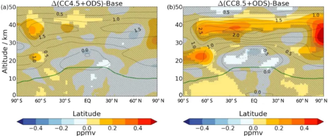
Generally, changes in annual and zonal mean ozone and temperature for the combined-forcing runs1(CC4.5+ODS), 1(CC8.5+ODS),1(CC4.5+O3pre),1(CC8.5+O3pre) and 1(ODS+O3pre) can be closely reproduced from summing changes in the respective single-forcing runs.
The exception is the ozone response in1(CC8.5+ODS), in which two regions of small, but statistically significant, non-additivities are found (shading, Fig. 3b). The first is lo-cated in the upper stratosphere, where the response to climate change and reduced ODSs reinforce one another (Chipper-field and Feng, 2003). Here, the simulated increase in ozone is around 0.2 ppmv greater than that calculated from a linear addition of the1CC8.5 and1ODS perturbations. The effect is caused by a change in the temperature dependence of cat-alytic ozone loss (positive if evaluated by d ln[O3]/dT−1as
in Haigh and Pyle, 1982) with a reduction in halogen load-ing. This is essentially the same effect found by Haigh and Pyle (1982) in their experiment combining a doubling in CO2
Figure 3.Changes in annual and zonal mean ozone (ppmv, contours) from Base to two combined-forcing runs:(a)1(CC4.5+ODS) and
(b) 1(CC8.5+ODS). The shading indicates the amount by which the response deviates from additivity (i.e. the difference between the combined-forcing experiment and the sum of the individual-forcing cases). Areas where the non-additive component of the response is not significant at the 95 % level according to a Student’sttest are hatched out. The solid green line indicates the thermal tropopause of the Base run.
The second region where the1(CC8.5+ODS) response is non-additive is the lower stratosphere at around 60◦S; this can be ascribed to a non-additivity in the amount of chlo-rine activated through heterogeneous reactions of reservoir species (ClONO2 and HCl) on PSCs and sulfate aerosols.
This can be rationalised by considering the rate of these re-actions, which is proportional to the product of PSC/aerosol surface area density (SAD) and [Cl reservoir]. Thus, when [Cl reservoir] is low (e.g. due to the lower Cly loadings in
1ODS), increases in the rate of reaction due to increases in SAD (e.g. due to cooling under climate change) are smaller. Therefore, in1(CC8.5+ODS), reductions in active chlorine (ClOx) are greater than expected from their separate effects,
and hence the ozone concentration is higher. These effects occur primarily at the edge of the vortex, where cooling un-der climate change leads to greater PSC formation and hence ClOxconcentrations. In contrast, in the cold core of the
vor-tex, cooling under climate change does not greatly affect PSC areas, since temperatures are already below the PSC forma-tion threshold in the Base experiment.
For both the upper and lower stratosphere, the magni-tude of the deviation from additivity scales with the amount of stratospheric cooling. Thus, the effects are present to a much lesser extent when combining 1ODS with1CC4.5 (Fig. 3a), which causes around a third of the stratospheric cooling found under1CC8.5 (Fig. 1b and d).
Note that scenarios in which CH4 or N2O are changed
in the chemistry scheme have not been explored. If such perturbations were combined with1ODS, non-additive re-sponses would be expected since both CH4and N2O control
chlorine partitioning (through CH4+Cl→HCl+CH3 and
NO2+ClO+M→ClONO2+M, respectively) (e.g.
Flem-ing et al., 2011; Portmann et al., 2012; Meul et al., 2015). Overall, the stratospheric changes are largely as expected from theory and previous model studies (e.g. Haigh and Pyle,
1982; Jonsson et al., 2004; Austin et al., 2010; Eyring et al., 2013; Meul et al., 2014). Insight into the impact of methane changes, which are not explored here, can also be garnered from previous literature (Randeniya et al., 2002; Stenke and Grewe, 2005; Portmann and Solomon, 2007; Fleming et al., 2011; Revell et al., 2012). These studies conclude that the stratospheric ozone response to increased methane results from a combination of increased HOx-catalysed destruction
(upper stratosphere), enhanced production through smog-like chemistry (lower stratosphere), and reduced losses due to water-vapour-induced cooling and reductions in [ClOx].
Overall, Revell et al. (2012) find positive linear relationships between end of 21st century surface methane abundances and stratospheric column ozone across the four RCPs in the NIWA-SOCOL CCM.
We have demonstrated that the stratosphere is not strongly influenced by chemical changes in the free troposphere in these experiments. However, changes in stratospheric com-position and dynamics might have important impacts on the troposphere. To determine the extent of these impacts, the next section provides a detailed analysis of the troposphere.
4 Tropospheric ozone
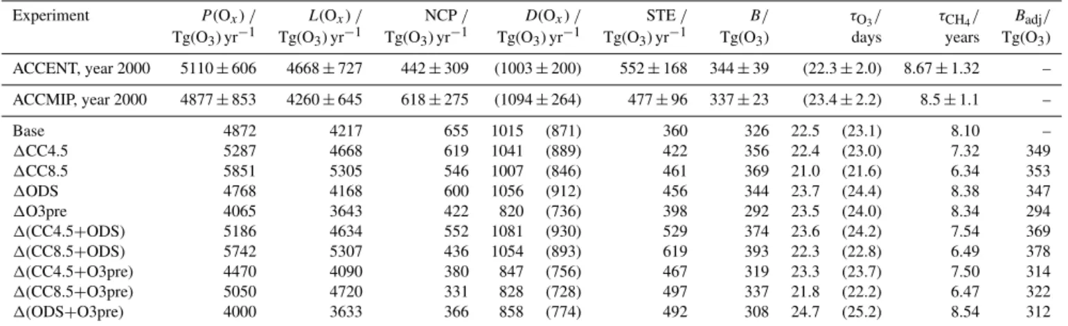
ex-Table 2.Tropospheric Oxbudget for the experiments detailed in Table 1. The definition of Oxemployed here is given in the Introduction.
Also reported is the tropospheric lifetime of ozone (τO3) and whole atmosphere lifetime of methane (τCH4). The latter includes loss by
tropospheric OH (diagnosed by the model), a soil sink (lifetime 160 years) and a stratospheric sink (lifetime 120 years). The final column shows values of the ozone burden after adjusting to account for methane feedbacks (Badj) (see Sect. 4.3 for details). Two sets of multi-model
means for the year 2000 are included for comparison with the Base run: ACCENT values (first row) are taken from or calculated from data in Stevenson et al. (2006), and ACCMIP (second row) from Young et al. (2013) for all terms exceptτCH4, which has been calculated from the
tropospheric methane lifetimes reported in Naik et al. (2013). Note that, in this study, theD(Ox) term totals dry deposition of ozone (listed
in brackets) plus deposition of those reactive nitrogen compounds that are classed as Ox, whereas the ACCENT and ACCMIP studies only
report the former. The same applies in the calculation ofτO3.
Experiment P(Ox)/ L(Ox)/ NCP/ D(Ox)/ STE/ B/ τO3/ τCH4/ Badj/
Tg(O3) yr−1 Tg(O3) yr−1 Tg(O3) yr−1 Tg(O3) yr−1 Tg(O3) yr−1 Tg(O3) days years Tg(O3) ACCENT, year 2000 5110±606 4668±727 442±309 (1003±200) 552±168 344±39 (22.3±2.0) 8.67±1.32 – ACCMIP, year 2000 4877±853 4260±645 618±275 (1094±264) 477±96 337±23 (23.4±2.2) 8.5±1.1 –
Base 4872 4217 655 1015 (871) 360 326 22.5 (23.1) 8.10 –
1CC4.5 5287 4668 619 1041 (889) 422 356 22.4 (23.0) 7.32 349
1CC8.5 5851 5305 546 1007 (846) 461 369 21.0 (21.6) 6.34 353
1ODS 4768 4168 600 1056 (912) 456 344 23.7 (24.4) 8.38 347
1O3pre 4065 3643 422 820 (736) 398 292 23.5 (24.0) 8.34 294
1(CC4.5+ODS) 5186 4634 552 1081 (930) 529 374 23.6 (24.2) 7.54 369
1(CC8.5+ODS) 5742 5307 436 1054 (893) 619 393 22.3 (22.8) 6.49 378
1(CC4.5+O3pre) 4470 4090 380 847 (756) 467 319 23.3 (23.7) 7.50 314
1(CC8.5+O3pre) 5050 4720 331 828 (728) 497 337 21.8 (22.2) 6.47 322
1(ODS+O3pre) 4000 3633 366 858 (774) 492 308 24.7 (25.2) 8.54 312
periments; for multi-model means (Stevenson et al., 2006; Naik et al., 2013; Young et al., 2013), errors give the inter-model range as 1σ.
4.1 Year 2000 tropospheric Oxbudget
The global and annual mean Ox budget of the troposphere
for all experiments is shown in Table 2. Multi-model mean values from the ACCENT ensemble (Stevenson et al., 2006) are included for comparison to the Base run. Values for the more recent ACCMIP ensemble are also shown, with the caveat that only six of those models diagnosed the Ox
budget, although all 15 models diagnosed the ozone bur-den and methane lifetime (Naik et al., 2013; Young et al., 2013). For most terms, the Base run compares favourably with the ACCENT and ACCMIP results. Chemical produc-tion (P(Ox)), chemical loss (L(Ox)) and deposition are well
within 1σ of the multi-model means; we compare the dry deposition of ozone here (see Table 2) but consider depo-sition of all Ox (D(Ox)) hereafter. However, the inferred
STE of 360±14 Tg(O3) yr−1 is lower than observational
estimates, which range between 450 and 550 Tg(O3) yr−1
(e.g. Gettelman et al., 1997; Olsen et al., 2001, 2013), and the ACCENT and ACCMIP means of 552±168 and 477±96 Tg(O3) yr−1, respectively. Nevertheless, a
compar-ison to these model intercomparcompar-isons is likely to be inad-equate in this case – only three out of the six ACCMIP models that reported STE contained full stratospheric chem-istry (Lamarque et al., 2013; Young et al., 2013), while al-most none of the ACCENT models contained this represen-tation. In addition, some models altered the stratospheric
up-per boundary condition to match observational constraints, whereas STE cannot be predetermined in such a way in the UM-UKCA scheme.
The Base ozone burden of 326±2 Tg(O3) is close to
the ACCENT and ACCMIP ensemble means (344±39 and 337±23 Tg(O3), respectively). Note that the UM-UKCA
budgets are calculated using the monthly mean thermal tropopause in contrast to the two model intercomparisons, which used a chemical tropopause defined by the 150 ppbv contour of ozone. However, the Ox budget terms in the
Base run do not differ greatly between the two definitions. At most, relative differences reach 2 % for both the bur-den (7 Tg(O3) lower) and STE (8 Tg(O3) yr−1greater) when
comparing the chemical with the thermal tropopause. Fur-thermore, observations obtained between 2004 and 2010 from the Ozone Monitoring Instrument (OMI) and Mi-crowave Limb Sounder (MLS) (Ziemke et al., 2011) indicate a climatological, total ozone burden of 295 Tg(O3) between
the latitudes 60◦S and 60◦N, which compares well with the value of 298 Tg(O3) in the Base run.
Effects of the year 2100 perturbations on the ozone burden are now discussed, and the underlying causes investigated.
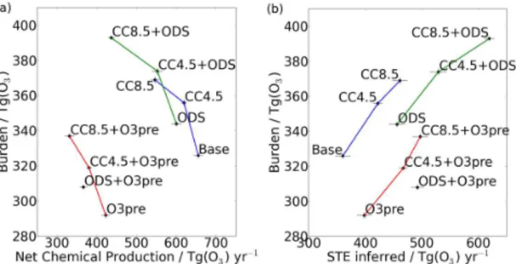
4.2 Ozone burden
Figure 4.Tropospheric ozone burden against(a)NCP and(b)STE. Connecting lines are drawn between experiments which differ only in their climate states. Error bars denote the 5–95 % confidence in-terval, calculated as±1.96 times the standard error in the mean.
or production rate (the “turnover flux”), so changes in these quantities are also considered. Note that, to ensure a phys-ically consistent definition of the troposphere, the height of the tropopause is allowed to change in response to the climate perturbations in these experiments. Therefore, under climate change, a rising of the tropopause contributes to an increase in the ozone burden.
Reductions in emissions of ozone precursors lower the ozone burden; for the 1O3pre experiment, a decrease of 34±2 Tg(O3) (10.4 %) is found despite an increase inτO3 (Sect. 4.6). This is driven mainly by a decrease in chemi-cal ozone production (Sect. 4.4), causing considerable reduc-tions in both the turnover flux (−769 Tg(O3) yr−1) and NCP
(−233 Tg(O3) yr−1, Fig. 4a). This can be compared to a very
small increase in STE of 38 Tg(O3) yr−1(Fig. 4b) and a
re-duction inD(Ox) of 195 Tg(O3) yr−1(Table 2).
In contrast, the ozone burden increases under cli-mate change and lower ODS concentrations. For the single-forcing experiments, the increases are 30±2 Tg(O3)
(9.2 %) (1CC4.5), 43±2 Tg(O3) (13.2 %) (1CC8.5) and
18±2 Tg(O3) (5.5 %) (1ODS). For1CC4.5/1CC8.5, these
are largely due to increases in the turnover flux of 477/1080 Tg(O3) yr−1, which occur alongside no change
in τO3 in 1CC4.5 and a reduction in τO3 in 1CC8.5 (Table 2, Sect. 4.6). For 1ODS, there is a negligible change in the turnover flux (−8 Tg(O3) yr−1), but the ozone
burden is increased as a result of higher τO3 (Table 2, Sect. 4.6). In all of these experiments, large increases in STE of 62/101/96 Tg(O3) yr−1(1CC4.5/1CC8.5/1ODS) play a
crucial role by increasing the ozone source and its life-time (Fig. 4b, Sect. 4.6). These are comparable to, or larger than, the respective reductions in NCP of 36, 109 and 55 Tg(O3) yr−1 (Fig. 4a).D(Ox) shows smaller changes of
26,−8 and 41 Tg(O3) yr−1, respectively (Table 2).
Banerjee et al. (2014) highlighted the importance of changes in LNOx under climate change for increasing the
ozone burden and hence opposing the effects of projected reductions in ozone precursors. The results presented here
Fig. 4). Furthermore, through increased STE, reduced ODSs also act to oppose the effects of1O3pre (Table 2, Fig. 4).
The response of the tropospheric budget terms to cli-mate change is qualitatively consistent with results from most other model studies, which find reductions in NCP, in-creases in STE and inin-creases in the turnover flux under var-ious climate forcing scenarios (e.g. Stevenson et al., 2006; Zeng et al., 2008; Kawase et al., 2011; Morgenstern et al., 2013; Young et al., 2013). For the ozone burden, Kawase et al. (2011) also find increases under RCP4.5 and 8.5 in sensi-tivity tests that are similar to the1CC4.5 and1CC8.5 runs of this study. However, this response is likely to be model-dependent. For example, the ACCENT inter-model range in future changes in the ozone burden encompasses both in-creases and dein-creases for the same climate forcing scenario (Stevenson et al., 2006).
Note that we have not performed simulations that include all forcings. For the ACCMIP ensemble mean, the combined impact of all forcings on the ozone burden between 2000 and 2100 was found to be a decrease of 7 % (RCP4.5) and an increase of 18 % (RCP8.5), which is dominated by the effects of NOx/CO/NMVOC emission reductions and an increase in
methane, respectively (Young et al., 2013).
4.3 Implications of methane adjustments for the ozone burden
The tropospheric ozone burden is also affected by the method with which the methane boundary condition is applied in the model. All experiments include a uniform fixed lower boundary condition of 1.75 ppmv for methane, which effec-tively fixes its abundance throughout the troposphere. Thus any changes in OH essentially do not affect methane concen-trations, nor are any subsequent feedbacks captured. This in-cludes the influence of methane on its own abundance (Isak-sen and Hov, 1987) as well as on ozone.
The feedback factor,f (e.g. Fuglestvedt, 1999), gives a measure of the influence of methane on its own lifetime, and has previously been estimated to be 1.52 for this model (Banerjee et al., 2014). Following the methodology in that study and references therein, the amount of methane and ozone that would be simulated at equilibrium if methane were allowed to evolve freely have been calculated using the whole atmosphere methane lifetime (τCH4) reported in Ta-ble 2; corresponding equilibrium ozone burdens are reported in the final column.
The estimated equilibrium ozone burdens are 7 and 16 Tg(O3) smaller than simulated in the 1CC4.5 and
1CC8.5 experiments, respectively. In contrast, only a 3 and 2 Tg(O3) increase in ozone burden compared to
ex-periments, respectively. Therefore, when considering the ef-fects of methane adjustments, the extent to which climate change counters the impact of 1O3pre on the ozone bur-den is somewhat reduced, while the extent to which1ODS counters1O3pre is slightly increased. Nonetheless, the qual-itative conclusions remain unchanged.
Having discussed changes in the ozone burden, the fol-lowing subsection further explores the tropospheric Ox
bud-get and investigates the underlying causes of the changes in NCP and STE.
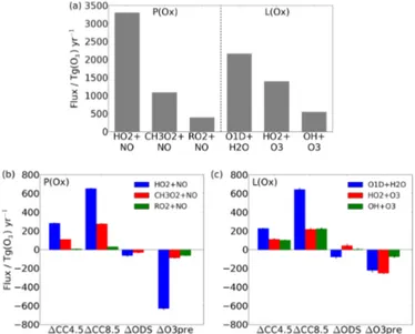
4.4 Chemical production and loss
To explore changes in NCP, Fig. 5 shows mean values for the Base experiment and the changes due to each type of perturbation in the primary Ox chemical production
(HO2+NO, CH3O2+NO and RO2+NO, where RO2 is a
generic peroxy radical not including HO2 or CH3O2) and
loss (O(1D)+H2O, HO2+O3 and OH+O3) routes.
To-gether, these constitute 98 and 97 % of total chemical pro-duction and loss of Ox, respectively.
Figure 4a shows that reductions in NCP are largest when emissions of ozone precursors are reduced. Figure 5b shows that this is driven by decreases in P(Ox), primarily through
the HO2+NO reaction. Mitigation of NOx emissions, and
hence a reduction in NO concentrations, directly drive the majority of this response. Reductions in NMVOC and, in particular, CO emissions also contribute by slowing down OH to HO2 conversion, thus reducing HO2concentrations.
Additionally, the decreases in ozone also act to reduce HOx
abundances. We do not quantify the relative importance of these separate drivers.
The impact of climate change reduces NCP in the exper-iments, as can be seen from each set of connecting lines in Fig. 4a; this is in qualitative agreement with recent multi-model studies (Stevenson et al., 2006; Young et al., 2013). This is the result of greater L(Ox), which dominates over a
smaller increase inP(Ox). GreaterL(Ox) occurs primarily
via increased O(1D)+H2O (Fig. 5c) as atmospheric
mois-ture content increases, and is a robust feamois-ture across models, although the magnitude will depend on the amplitude of tro-pospheric warming. Here, this is determined by the imposed SSTs and sea ice which are derived from a model that is part of the HadGEM2 family, known to lie on the upper end of the current modelled range of equilibrium climate sensitivities (Andrews et al., 2012). GreaterP(Ox) occurs mainly due to
increasedLNOxassociated with changes in tropical
convec-tion (see Banerjee et al., 2014, for more details), although the importance of this effect relative to other drivers of Ox
pro-duction is expected to be highly model-dependent. The fluxes through HO2+NO and CH3O2+NO (Fig. 5b) thus increase
with climate change. Both P(Ox) andL(Ox) are amplified
for the larger RCP8.5 climate forcing.
Figure 4a also shows that there are consistent reductions in NCP under lower ODS concentrations. For the 1ODS
Figure 5. (a) Global tropospheric and annual mean fluxes in the Base run through the main channels for chemical production and loss of Ox. Differences between Base and the four
differ-ent types of perturbation are shown for chemical(b) production and (c) loss. These account for the changes in all runs that in-clude a particular type of perturbation; for example, the bars for
1CC4.5 represent the mean of the differences 1CC4.5−Base,
1(CC4.5+ODS)−1ODS and 1(CC4.5+O3pre)−1O3pre. The range of these calculated means is illustrated by whiskers on each bar.
experiment, NCP is reduced by 55 Tg(O3) yr−1 relative to
Base, with P(Ox) reduced (−104 Tg(O3) yr−1) more than
L(Ox) (−49 Tg(O3) yr−1). This result is strongly influenced
by changes in stratospheric ozone which lead to modifica-tions in tropospheric actinic fluxes and photolysis rates, with subsequent chemical feedbacks in the troposphere. P(Ox)
andL(Ox) are particularly sensitive to photolysis rates for
NO2 to NO (J(NO2)) and O3 to O(1D) (J(O3)). With
in-creases in stratospheric ozone (Figs. 1e and 2), J(O3) is
strongly reduced, but J(NO2) is largely unaffected.
Reduc-tions in J(O3) depress O(1D) abundances (not shown),
de-spite increases in tropospheric ozone. The reduction in O(1D) mixing ratio is largest in the extratropics and peaks at over 50 % in southern high latitudes, where the stratospheric ozone column is enhanced by∼80 DU in the annual mean (not shown), in contrast to the much smaller change in the tropics (see Fig. 2). With lower [O(1D)], the loss of Ox
through O(1D)+H2O is diminished (Fig. 5c). Loss through
HO2+O3is increased, however, due to the increase in
tro-pospheric ozone abundances. By contrast,P(Ox) is reduced
through two of its three major channels as a result of de-creases in ODSs (Fig. 5b). Following changes in strato-spheric column ozone, previous studies have shown that the sign of the HOx response follows that of J(O3) regardless
the overall changes in tropospheric ozone burden for the cli-mate change and ODS experiments. As previously described, changes in STE have an important role alongside modifica-tions to tropospheric chemical processes, and these are dis-cussed in the following section.
4.5 STE
4.5.1 Measures of STE and its influence on the troposphere
Although several metrics for STE exist (Hsu and Prather, 2014), the common approach of inferring STE from the other three terms of the Oxbudget is adopted here. In the Base
ex-periment, STE is calculated to be 360 Tg(O3) yr−1. STE may
be altered by changes in the residual circulation and two-way mixing (which collectively characterise the BDC) (Plumb, 2002), and in the ozone distribution in the extratropical lower stratosphere.
The transformed Eulerian mean (TEM) residual vertical velocity (Andrews et al., 1987) and the total upward and downward residual mass fluxes across a fixed pressure sur-face (Rosenlof, 1995) are used as metrics for the strato-spheric circulation. Mass fluxes are calculated between all latitudes where there is net upward or downward motion, respectively. The upward mass flux at 70 hPa is used as a measure for the overall strength of the residual circula-tion (SPARC CCMVal, 2010). The downward mass flux at 100 hPa is used as an indicator for the STE of air, although more accurate measures exist (for a fuller discussion see Rosenlof and Holton, 1993; Holton et al., 1995; Rosenlof, 1995; Yang and Tung, 1996).
The climatological, annual mean upward mass flux at 70 hPa in the Base experiment is 7.9×10⁹kg s−1. For
com-parison, the ERA-Interim reanalysis data (Dee et al., 2011) and most models within the Chemistry-Climate Model Val-idation project (CCMVal-2) indicate a value of around 6×10⁹kg s−1 (Butchart et al., 2011); the residual
circula-tion is therefore∼33 % stronger in the UM-UKCA model. Changes in the residual circulation in the single-forcing ex-periments will be linked qualitatively to changes in STE in Sect. 4.5.2.
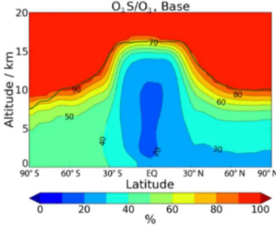
While quantifying the global and annual net flux of ozone into the troposphere is useful for understanding changes in the global burden of tropospheric ozone, to study the im-pacts on the distribution of ozone in the troposphere, we use the stratospheric ozone tracer, O3S (see Sect. 2.2). Note that
the amount and distribution of O3S in the troposphere
de-pends on its tropospheric lifetime and transport, in addition to transport from the stratosphere. Figure 6 shows the rel-ative contribution of O3S to the annual mean ozone field in
Figure 6.The zonal and annual mean contribution of O3S to ozone in the Base simulation. The solid green line indicates the thermal tropopause of the Base run.
the Base experiment. The contribution is lowest (20 %) in the equatorial region, where upward transport takes place. The contribution is greater in the extratropics, particularly so in the Southern Hemisphere (SH), where other sources of ozone are relatively weak.
4.5.2 Changes in STE
The residual circulation, as measured by the upward mass flux at 70 hPa, is projected to strengthen under climate change by all climate models (e.g. Butchart et al., 2006, 2010; SPARC CCMVal, 2010; Hardiman et al., 2013). The UM-UKCA model also shows this behaviour: Fig. 7a shows an increase of 10 % (1CC4.5) and 27 % (1CC8.5) in the annual mean. The latter result is comparable to the CMIP5 multi-model mean increase for the RCP8.5 scenario of 32 % between 2000 and 2100, extrapolated from the linear rate of change found between 2006 and 2099 (Butchart, 2014).
The BDC consists of two distinct branches, commonly re-ferred to as the deep and shallow branches (Plumb, 2002). Both branches strengthen under climate change in these ex-periments, which is in agreement with other recent studies (Hardiman et al., 2013; Lin and Fu, 2013). The downward mass flux at 100 hPa increases by 11 % in the SH and 21 % in the NH in1CC4.5, and by 37 and 42 %, respectively, in 1CC8.5 (Fig. 7b and c); these are the main contributors to the increases in global STE of 62 and 101 Tg(O3) yr−1,
re-spectively. This result is supported by Collins et al. (2003), Zeng and Pyle (2003) and Zeng et al. (2010), who isolated the effects of circulation changes on STE in a future climate. Figure 8 shows absolute changes in O3S and ozone
be-tween Base and selected experiments (1CC8.5,1ODS and 1(CC8.5+ODS)), as well as changes in tropospheric ozone for comparison. Increases in O3S occur particularly in the
Figure 7. Changes in total (a) upward (b) downward (SH) and
(c)downward (NH) mass fluxes at 70 hPa (blue bars) and 100 hPa (red bars) for the single-forcing experiments relative to Base. Er-ror bars indicate the 5–95 % confidence interval, calculated as
±1.96 times the standard error in the mean of the change.
contributes to this response. This does not preclude another important contribution from more efficient isentropic stirring across the tropopause (as suggested by the idealised model study of Orbe et al., 2013). This effect may be particularly important for ozone, which has a large concentration gradi-ent across the tropopause.
The peak O3S increase in 1CC8.5 is greater in the NH
subtropics (7 ppbv) than in the SH (5 ppbv). Despite this, the hemispheric asymmetry in the tropospheric ozone change (Fig. 8b) is in the opposite sense, due to a greater contribution fromLNOx-produced ozone in the SH. Using a simulation
in which climate is allowed to vary according to the RCP8.5 scenario, but in whichLNOxis fixed to Base values (detailed
in Banerjee et al., 2014), we deduce that the change in O3S
under climate change can be as large as 30/50 % (SH/NH) of
the increase in ozone due to increases inLNOx in the
sub-tropics.
Consistent with Palmeiro et al. (2014), Lin and Fu (2013) and Oberländer et al. (2013), ozone recovery in the1ODS experiment is associated with a weakening of the SH deep branch of the BDC during austral summer. In this model, a weakening of the NH deep branch is also simulated. Con-comitantly, the upward mass flux at 70 hPa is reduced by 4.5 % (Fig. 7a). However, the relative mass flux anomalies in the lowermost stratosphere are small, with the downward mass flux at 100 hPa decreasing by only 1.8/4.1 % (SH/NH) (Fig. 7b and c).
While the residual circulation is not strongly af-fected in the 1ODS experiment, STE still increases by 96 Tg(O3) yr−1, a change that is approximately equal to that
for1CC8.5. This is attributable to the large increase in extra-tropical lower stratospheric ozone (Fig. 1e). Increased trans-port of stratospheric ozone into the extratropical troposphere is evident from the change in O3S for 1ODS (Fig. 8c).
Greater O3S amounts are particularly prominent in the NH,
where, despite the smaller absolute increase in lower strato-spheric ozone, the residual circulation is stronger and the net stratosphere to troposphere mass flux of air is larger than in the SH (see also Schoeberl, 2004). The corresponding change in ozone (Fig. 8d) strongly resembles that of O3S,
suggest-ing that most of the tropospheric ozone change is driven by increased STE.
Figure 7 shows that the1O3pre perturbation leads to no significant change in the stratospheric residual circulation; neither is extratropical lower stratospheric ozone greatly af-fected (Fig. 1g). The amount of ozone entering the tropo-sphere from the stratotropo-sphere is therefore similar in the Base and1O3pre experiments. The small increase in net STE of 38 Tg(O3) yr−1 could instead be due to a reduction in Ox
transport from the troposphere into the tropical lower strato-sphere, but the effect is small enough to cause no statisti-cally significant change in tropical lower stratospheric ozone amounts (Fig. 1g).
Considering the entire set of experiments, a large range in STE of 360–619 Tg(O3) yr−1 is simulated (Fig. 4b), the
upper bound of which is found in the1(CC8.5+ODS) ex-periment. Interestingly, climate change and ODSs have their greatest impact on O3S in different regions. Climate change
has its largest effect on the subtropical upper troposphere (Fig. 8a), and ODSs on the middle/high latitudes (Fig. 8c). Consequently, there are increases in O3S throughout much of
the troposphere in the1(CC8.5+ODS) experiment (Fig. 8e). It is notable that, for this experiment, the effect of increased humidity on lowering ozone dominates only in a small region of the lowermost tropical troposphere (Fig. 8f), in contrast to the experiment with climate change alone (Fig. 8b), where the offset is much more widespread.
present-Figure 8.Changes in annual and zonal mean O3S (first column) and ozone (second column) mixing ratios (ppbv) from Base to a selection of experiments,1CC8.5,1ODS and1(CC8.5+ODS). The solid green line indicates the thermal tropopause of the Base run. Strong reductions in O3S and ozone occur near the tropopause under climate change because of a lifting of the tropopause, which introduces tropospheric
(ozone-poor) air into this region.
day (year 2000). If this relationship holds more generally across models, we might expect future changes in STE for other models to be larger than those found in this study, since the baseline STE in UM-UKCA is on the lower end of the contemporary modelled range. Indeed, increases in STE under climate change in this study (i.e. from a lower baseline) are smaller than found by Kawase et al. (2011) between the years 2005 and 2100 in similar sensitivity ex-periments. For scenarios which isolate the impact of strato-spheric ozone recovery under declining ODS loadings, the absolute changes found here are similar to their results: 96 Tg(O3) yr−1 (1ODS in this study) and 91 Tg(O3) yr−1
(Kawase et al., 2011). This suggests that the uncertainty in future changes in STE mostly lies in the effects of climate change and stratospheric circulation.
4.6 Effects on ozone lifetime
to-tal Ox loss (chemical and deposition). τO3 in the Base ex-periment closely matches the ACCENT and ACCMIP mean values; note that, for this comparison, only the deposition of ozone, and not Ox, is considered in the τO3 definition (Ta-ble 2, bracketed values). Changes about a baseline τO3 of 22.5±0.1 days (Table 2) as a result of each type of perturba-tion are now considered.
Figure 9 shows the ozone burden against τO3 for all ex-periments. For the 1O3pre perturbation, τO3 increases by 1.0±0.1 days (4.4 %). In this experiment, the largest reduc-tion in ozone occurs near the surface, where its lifetime is low. Thus, removing ozone in this region further increases τO3 (the deposition term of the Oxbudget is lower by, on av-erage, 199 Tg(O3) yr−1 in all runs which include1O3pre).
τO3 is also affected by changes in the amount of HOx and its partitioning. Mitigation of surface NOxemissions reduces
total HOx(through ozone), which increasesτO3. The reduc-tion in emissions favours HO2 over OH, which drives a
re-duction inτO3 since loss of ozone to HO2is greater than to OH (see Fig. 5a). This is only important in the lowermost troposphere since the NOxlifetime is short near the surface
and the impact onτO3 through this mechanism is thus small (Wang and Jacob, 1998). An increase in τO3 comes from the decrease in CO (in particular) and NMVOC emissions, which favours HOxpartitioning towards OH, as discussed in
Sect. 4.4.
A decrease in τO3 of 0.1±0.1 days (0.4 %) (1CC4.5) and 1.5±0.1 days (6.7 %) (1CC8.5) is found under climate change, predominantly as a result of greater water-vapour-induced loss of ozone. This is counteracted by increases in LNOx and STE, which increase ozone in the upper
tropo-sphere where its lifetime is long. For 1CC8.5, the water vapour effect dominates leading to the largest decrease inτO3 within the entire set of experiments (Fig. 9).
In the1ODS experiment,τO3 increases by 1.2±0.1 days (5.3 %) as a result of decreases in O(1D), OH and HO
2
amounts, especially at middle and high latitudes, as discussed in Sect. 4.4. Enhanced STE augments this effect.
Hence, in terms of τO3, the effects of climate change at RCP8.5 oppose those of 1O3pre, while 1ODS enhances them. The largest increase in lifetime of 2.2±0.1 days is cal-culated for 1(ODS+O3pre), which outweighs the decrease in 1CC8.5 (1.5±0.1 days). The colour-coded arrows in Fig. 9 denote the changes in τO3 when a particular type of perturbation is added, either in isolation or in combination. The fact that all arrows for a particular type of perturbation (i.e. those of a particular colour) follow approximately the same path indicates that the changes are linearly additive.
4.7 Tropospheric additivity
We now consider the additivity in the tropospheric ozone response for the combined-forcing experiments. Figure 10 compares modelled values of NCP, STE and the ozone bur-den for the combined-forcing experiments with those
ex-Figure 9.Tropospheric ozone burden against the ozone lifetime. Arrows indicate the impact of climate change at RCP4.5 (blue) and RCP8.5 (red), reduced ODS loadings (green) and reduced ozone precursor emissions (magenta). Error bars indicate the 5–95 % con-fidence interval, calculated as±1.96 times the standard error in the mean.
Figure 10.Correlations in(a)NCP,(b)STE and(c)the ozone bur-den between the combined-forcing experiments and those expected from a linear addition of changes in the single-forcing experiments relative to Base. The 1 : 1 lines are drawn in blue. Error bars indi-cate the 5–95 % confidence interval calculated as±1.96 times the standard error in the mean.
pected from a linear addition of changes in the respective single-forcing experiments. It is evident that, generally, the changes match those expected assuming additivity.
sphere into the troposphere in the SH and, to a lesser ex-tent, in the NH. This is qualitatively expected since an in-crease in the strength of the stratospheric circulation (due to climate change) under greater background ozone (due to re-duced ODS amounts) leads to a greater increase in STE than expected from the sum of the two separate effects. The im-pact is largest in the SH, where increases in lower strato-spheric ozone are largest.
The non-additive change in ozone in the SH lower strato-sphere for this experiment (Fig. 3b) might further contribute to the non-additive change in STE, although we cannot verify such an assumption due to the relevant diagnostics not being available and further sensitivity tests would be required.
Non-additivity in1(CC8.5+ODS) is also evident in NCP (Fig. 10a), which is found to be 55 Tg(O3) yr−1 less than
expected. The response is driven by chemical loss rather than production: greater loss occurs directly as a result of STE-derived increases in ozone (relative to the additive re-sponse). To a great extent, the larger loss counters increased STE, such that the change in the global ozone burden for 1(CC8.5+ODS) (Fig. 10c) is close to the expected response, demonstrating the strong buffering that takes place in re-sponse to increases in tropospheric ozone.
5 Conclusions
This study has explored the impacts of future climate change, reductions in ozone-depleting substances (ODSs) and in non-methane ozone precursor emissions on global ozone and, in particular, on the tropospheric budget of odd oxygen (Ox). Time-slice experiments representing conditions for the
years 2000 and 2100 were performed with the UM-UKCA chemistry–climate model (CCM), in a configuration that contains a comprehensive description of both stratospheric and tropospheric chemistry. This allowed an investigation of the consequences of future changes in stratospheric chem-istry and dynamics for the tropospheric Oxbudget.
The principal results regarding the stratosphere are as fol-lows:
1. Changes in ozone and temperature are in qualitative agreement with previous literature.
2. For simulations in which two types of perturbation are combined, changes in ozone can generally be repro-duced by the sum of changes in the appropriate single-forcing experiments. The only exception arises when combining a large climate forcing (RCP8.5) with the effects of ODSs, for which there is detectable non-additivity in the upper stratosphere and Southern Hemi-sphere lower stratoHemi-sphere.
Figure 11.As for Fig. 3, but showing the change in O3S (ppbv,
contours) from Base to1(CC8.5+ODS) as well as the deviation from additivity (shading) of the response. Areas where the shading is not significant at the 95 % level according to a two-tailed Stu-dent’sttest are hatched out. The solid green line indicates the ther-mal tropopause of the Base run.
The principal results regarding the troposphere are the fol-lowing:
1. The global tropospheric ozone burden decreases with projected reductions in ozone precursor emissions as part of air quality controls, but this effect is opposed by future changes in climate and ODSs; some combina-tion of these processes will determine future changes in tropospheric oxidising capacity and background surface ozone.
2. Increases in stratosphere–troposphere exchange (STE) of Ox primarily result from a strengthened Brewer–
Dobson circulation under climate change and from in-creases in lower stratospheric ozone abundances under reduced ODSs.
3. The increases in STE act to increase ozone most in the subtropical (climate change) and extratropical (ODS changes) upper troposphere; this should have implica-tions for the climate feedback since the upper tropo-sphere is a key region for ozone as a radiative forcing agent.
4. The enhancements in STE offset concomitant reduc-tions in net chemical production and act to increase the global tropospheric ozone burdens under climate change and reduced ODSs.
6. Changes in the tropospheric Ox budget terms when
combining two types of perturbation can generally be reproduced by summing the effects of the separate per-turbations. Combining changes in climate (RCP8.5) and ODSs leads to a non-additive change in STE, but the ef-fect on the ozone burden is strongly buffered.
The sensitivity tests in this study have investigated the ef-fects of some, but not all, of the key drivers of ozone un-der selected scenarios. For example, the future evolution of methane is highly uncertain and its chemical effects have not been examined here. CCM studies that have imposed increases in methane according to the RCP scenarios show large increases in tropospheric ozone, particularly at RCP8.5, which would greatly oppose the effects of emission controls on global, tropospheric ozone (e.g. Young et al., 2013; Revell et al., 2015).
The base climate state, climate sensitivity (incorporated here through the imposed sea surface temperatures), chem-ical complexity and parameterisations of processes such as lightning NOx emissions may all contribute to inter-model
differences and uncertainties in projections of future ozone. However, although the quantitative results of this study are likely to be specific to UM-UKCA, the significance of the stratosphere in determining future changes in tropospheric ozone through STE is clear. The results therefore empha-sise the need for a good representation of STE in CCMs to simulate future tropospheric ozone. While models with sim-plified stratospheric ozone chemistry are unlikely to repre-sent STE accurately (Olsen et al., 2013), this study achieves greater fidelity in its representation through the use of a CCM which contains a relatively sophisticated description of stratospheric and tropospheric chemistry and dynamics. Nonetheless, better constraints on observed estimates of STE are required to deduce whether modelled values are real-istic; it is hoped that, with continued satellite observations of ozone in the upper stratosphere–lower stratosphere (e.g. Livesey et al., 2008), this uncertainty can be reduced.
Acknowledgements. We thank the ERC for support under the
ACCI project, project no. 267760. A. C. Maycock was supported by a postdoctoral fellowship from the AXA Research Fund. A. T. Archibald was supported by a fellowship from the Herchel Smith Foundation. This work made use of the facilities of HECToR, the UK’s national high-performance computing service, which was provided by UoE HPCx Ltd at the University of Edinburgh, Cray Inc and NAG Ltd, and funded by the Office of Science and Technology through EPSRC’s High End Computing Programme. This work also used the ARCHER UK National Supercomputing Service (http://www.archer.ac.uk).
Edited by: J. West
References
Andrews, D. G., Holton, J. R., and Leovy, C. B.: Middle Atmo-sphere Dynamics, Academic Press, San Diego, USA, 1987. Andrews, T., Gregory, J. M., Webb, M. J., and Taylor, K. E.:
Forcing, feedbacks and climate sensitivity in CMIP5 coupled atmosphere-ocean climate models, Geophys. Res. Lett., 39, L09712, doi:10.1029/2012GL051607, 2012.
Austin, J., Scinocca, J., Plummer, D., Oman, L., Waugh, D., Akiyoshi, H., Bekki, S., Braesicke, P., Butchart, N., Chipperfield, M., Cugnet, D., Dameris, M., Dhomse, S., Eyring, V., Frith, S., Garcia, R. R., Garny, H., Gettelman, A., Hardiman, S. C., Kin-nison, D., Lamarque, J. F., Mancini, E., Marchand, M., Michou, M., Morgenstern, O., Nakamura, T., Pawson, S., Pitari, G., Pyle, J., Rozanov, E., Shepherd, T. G., Shibata, K., Teyssèdre, H., Wil-son, R. J., and Yamashita, Y.: Decline and recovery of total col-umn ozone using a multimodel time series analysis, J. Geophys. Res.-Atmos., 115, D00M10, doi:10.1029/2010JD013857, 2010. Banerjee, A., Archibald, A. T., Maycock, A. C., Telford, P., Abra-ham, N. L., Yang, X., Braesicke, P., and Pyle, J. A.: Lightning NOx, a key chemistry–climate interaction: impacts of future
cli-mate change and consequences for tropospheric oxidising capac-ity, Atmos. Chem. Phys., 14, 9871–9881, doi:10.5194/acp-14-9871-2014, 2014.
Butchart, N.: The Brewer–Dobson circulation, Rev. Geophys., 52, 157–184, doi:10.1002/2013RG000448, 2014.
Butchart, N., Scaife, A. A., Bourqui, M., Grandpré, J., Hare, S. H. E., Kettleborough, J., Langematz, U., Manzini, E., Sassi, F., Shibata, K., Shindell, D., and Sigmond, M.: Simulations of an-thropogenic change in the strength of the Brewer–Dobson cir-culation, Clim. Dynam., 27, 727–741, doi:10.1007/s00382-006-0162-4, 2006.
Butchart, N., Cionni, I., Eyring, V., Shepherd, T. G., Waugh, D. W., Akiyoshi, H., Austin, J., Brühl, C., Chipperfield, M. P., Cordero, E., Dameris, M., Deckert, R., Dhomse, S., Frith, S. M., Garcia, R. R., Gettelman, A., Giorgetta, M. A., Kinnison, D. E., Li, F., Mancini, E., Mclandress, C., Pawson, S., Pitari, G., Plummer, D. A., Rozanov, E., Sassi, F., Scinocca, J. F., Shibata, K., Steil, B., and Tian, W.: Chemistry-climate model simulations of twenty-first century stratospheric climate and circulation changes, J. Cli-mate, 23, 5349–5374, doi:10.1175/2010JCLI3404.1, 2010. Butchart, N., Charlton-Perez, A. J., Cionni, I., Hardiman, S. C.,
Haynes, P. H., Krüger, K., Kushner, P. J., Newman, P. A., Os-prey, S. M., Perlwitz, J., Sigmond, M., Wang, L., Akiyoshi, H., Austin, J., Bekki, S., Baumgaertner, A., Braesicke, P., Brühl, C., Chipperfield, M., Dameris, M., Dhomse, S., Eyring, V., Garcia, R., Garny, H., Jöckel, P., Lamarque, J.-F., Marc-hand, M., Michou, M., Morgenstern, O., Nakamura, T., Paw-son, S., Plummer, D., Pyle, J., Rozanov, E., Scinocca, J., Shep-herd, T. G., Shibata, K., Smale, D., Teyssèdre, H., Tian, W., Waugh, D., and Yamashita, Y.: Multimodel climate and variabil-ity of the stratosphere, J. Geophys. Res.-Atmos., 116, D05102, doi:10.1029/2010JD014995, 2011.
Chipperfield, M. P. and Feng, W.: Comment on: Stratospheric Ozone Depletion at northern mid-latitudes in the 21st cen-tury: The importance of future concentrations of greenhouse gases nitrous oxide and methane, Geophys. Res. Lett., 30, 1389, doi:10.1029/2002GL016353, 2003.
stratosphere-P., Kobayashi, S., Andrae, U., Balmaseda, M. A., Balsamo, G., Bauer, P., Bechtold, P., Beljaars, A. C. M., van de Berg, L., Bid-lot, J., Bormann, N., Delsol, C., Dragani, R., Fuentes, M., Geer, A. J., Haimberger, L., Healy, S. B., Hersbach, H., Hólm, E. V., Isaksen, L., Kållberg, P., Köhler, M., Matricardi, M., Mcnally, A. P., Monge-Sanz, B. M., Morcrette, J. J., Park, B. K., Peubey, C., de Rosnay, P., Tavolato, C., Thépaut, J. N., and Vitart, F.: The ERA-Interim reanalysis: Configuration and performance of the data assimilation system, Q. J. Roy. Meteor. Soc., 137, 553–597, doi:10.1002/qj.828, 2011.
Dessens, O., Zeng, G., Warwick, N., and Pyle, J.: Short-lived bromine compounds in the lower stratosphere; impact of climate change on ozone, Atmos. Sci. Lett., 10, 201–206, doi:10.1002/asl.236, 2009.
Eyring, V., Arblaster, J. M., Cionni, I., Sedláˇcek, J., Perlwitz, J., Young, P. J., Bekki, S., Bergmann, D., Cameron-Smith, P., Collins, W. J., Faluvegi, G., Gottschaldt, K.-D., Horowitz, L. W., Kinnison, D. E., Lamarque, J.-F., Marsh, D. R., Saint-Martin, D., Shindell, D. T., Sudo, K., Szopa, S., and Watanabe, S.: Long-term ozone changes and associated climate impacts in CMIP5 simulations, J. Geophys. Res.-Atmos., 118, 5029–5060, doi:10.1002/jgrd.50316, 2013.
Fels, S. B., Mahlman, J. D., Schwarzkopf, M. D., and Sin-clair, R. W.: Stratospheric Sensitivity to Perturbations in Ozone and Carbon Dioxide: Radiative and Dynamical Re-sponse, J. Atmos. Sci., 37, 2265–2297, doi:10.1175/1520-0469(1980)037<2265:SSTPIO>2.0.CO;2, 1980.
Fiore, A. M., Naik, V., Spracklen, D. V., Steiner, A., Unger, N., Prather, M., Bergmann, D., Cameron-Smith, P. J., Cionni, I., Collins, W. J., Dalsøren, S., Eyring, V., Folberth, G. A., Ginoux, P., Horowitz, L. W., Josse, B., Lamarque, J.-F., MacKenzie, I. A., Nagashima, T., O’Connor, F. M., Righi, M., Rumbold, S. T., Shindell, D. T., Skeie, R. B., Sudo, K., Szopa, S., Takemura, T., and Zeng, G.: Global air quality and climate, Chem. Soc. Rev., 41, 6663–6683, doi:10.1039/c2cs35095e, 2012.
Fleming, E. L., Jackman, C. H., Stolarski, R. S., and Douglass, A. R.: A model study of the impact of source gas changes on the stratosphere for 1850–2100, Atmos. Chem. Phys., 11, 8515– 8541, doi:10.5194/acp-11-8515-2011, 2011.
Fuglestvedt, J.: Climatic forcing of nitrogen oxides through changes in tropospheric ozone and methane; global 3-D model studies, Atmos. Environ., 33, 961–977, doi:10.1016/S1352-2310(98)00217-9, 1999.
Fuglestvedt, J. S., Johnson, J. E., and Isaksen, I. S. A.: Effects of reductions in stratospheric ozone on tropospheric chem-istry through changes in photolysis rates, Tellus, 46B, 172–192, doi:10.1034/j.1600-0889.1992.t01-3-00001.x-i1, 1994. Gettelman, A., Holton, J. R., and Rosenlof, K. H.: Mass fluxes of
O3, CH4, N2O and CF2Cl2in the lower stratosphere calculated
from observational data, J. Geophys. Res.-Atmos., 102, 19149– 19159, doi:10.1029/97JD01014, 1997.
Grewe, V.: Impact of Lightning on Air Chemistry and Climate, in: Lightning: Principles, Instruments and Applications, Review of Modern Lightning Research, edited by: Betz, H. D., Schu-mann, U., and Laroche, P., Springer Netherlands, available at:
C., Hinton, T. J., Jones, C. D., McDonald, R. E., McLaren, A. J., O’Connor, F. M., Roberts, M. J., Rodriguez, J. M., Woodward, S., Best, M. J., Brooks, M. E., Brown, A. R., Butchart, N., Dear-den, C., Derbyshire, S. H., Dharssi, I., Doutriaux-Boucher, M., Edwards, J. M., Falloon, P. D., Gedney, N., Gray, L. J., Hewitt, H. T., Hobson, M., Huddleston, M. R., Hughes, J., Ineson, S., In-gram, W. J., James, P. M., Johns, T. C., Johnson, C. E., Jones, A., Jones, C. P., Joshi, M. M., Keen, A. B., Liddicoat, S., Lock, A. P., Maidens, A. V., Manners, J. C., Milton, S. F., Rae, J. G. L., Rid-ley, J. K., Sellar, A., Senior, C. A., Totterdell, I. J., Verhoef, A., Vidale, P. L., and Wiltshire, A.: The HadGEM2 family of Met Of-fice Unified Model climate configurations, Geosci. Model Dev., 4, 723–757, doi:10.5194/gmd-4-723-2011, 2011.
Haigh, J. D. and Pyle, J. A.: Ozone perturbation experiments in a two–dimensional circulation model, Q. J. Roy. Meteor. Soc., 108, 551–574, doi:10.1002/qj.49710845705, 1982.
Hardiman, S. C., Butchart, N., and Calvo, N.: The morphology of the Brewer–Dobson circulation and its response to climate change in CMIP5 simulations, Q. J. Roy. Meteor. Soc., 140, 1958–1965, doi:10.1002/qj.2258, 2013.
Hauglustaine, D. A., Lathière, J., Szopa, S., and Folberth, G. A.: Future tropospheric ozone simulated with a climate-chemistry-biosphere model, Geophys. Res. Lett., 32, L24807, doi:10.1029/2005GL024031, 2005.
Holton, J. R., Haynes, P. H., McIntyre, M. E., Douglass, A. R., Rood, R. B., and Pfister, L.: Stratosphere-troposphere exchange, Rev. Geophys., 33, 403–439, doi:10.1029/95RG02097, 1995. Hossaini, R., Chipperfield, M. P., Dhomse, S., Ordóñez, C.,
Saiz-Lopez, A., Abraham, N. L., Archibald, A., Braesicke, P., Telford, P., Warwick, N., Yang, X., and Pyle, J.: Mod-elling future changes to the stratospheric source gas injection of biogenic bromocarbons, Geophys. Res. Lett., 39, L20813, doi:10.1029/2012GL053401, 2012.
Hsu, J. and Prather, M. J.: Is the residual vertical velocity a good proxy for stratosphere-troposphere exchange of ozone?, Geo-phys. Res. Lett., 41, 9024–9032, doi:10.1002/2014GL061994, 2014.
IPCC: Climate Change 2001: The Scientific Basis. Contribution of Working Group I to the Third Assessment Report of the Inter-governmental Panel on Climate Change, edited by: Houghton, J. T., Ding, Y., Griggs, D. J., Noguer, M., van der Linden, P. J., Dai, X., Maskell, K., and Johnson, C. A., Cambridge University Press, Cambridge, UK and New York, NY, USA, 2001. IPCC: Climate Change 2013: The Physical Science Basis.
Con-tribution of Working Group I to the Fifth Assessment Report of the Intergovernmental Panel on Climate Change, edited by: Stocker, T. F., Qin, D., Plattner, G.-K., Tignor, M., Allen, S. K., Boschung, J., Nauels, A., Xia, Y., Bex, V., and Midgley, P. M., Cambridge University Press, Cambridge, UK and New York, NY, USA, 2013.
Isaksen, I. S. A. and Hov, Ø.: Calculation of trends in the tropo-spheric concentration of O3, OH, CO, CH4and NOx, Tellus B,
39B, 271–285, doi:10.1111/j.1600-0889.1987.tb00099.x, 1987. Johnson, C. E., Collins, W. J., Stevenson, D. S., and Derwent, R.