ESP v2.0: enhanced method for exploring emission impacts of future scenarios in the United States – addressing spatial allocation

(1)

GMDD

8, 263–300, 2015

ESP v2.0: emission projection method

L. Ran et al.

Title Page

Abstract Introduction

Conclusions References

Tables Figures

◭ ◮

Back Close

Full Screen / Esc

Printer-friendly Version Interactive Discussion

Discussion

P

a

per

|

Discussion

P

a

per

|

Discussion

P

a

per

|

Discussion

P

a

per

|

Geosci. Model Dev. Discuss., 8, 263–300, 2015 www.geosci-model-dev-discuss.net/8/263/2015/ doi:10.5194/gmdd-8-263-2015

This discussion paper is/has been under review for the journal Geoscientific Model Development (GMD). Please refer to the corresponding final paper in GMD if available.

ESP v2.0: enhanced method for exploring

emission impacts of future scenarios in

the United States – addressing spatial

allocation

L. Ran1, D. H. Loughlin2, D. Yang1, Z. Adelman1, B. H. Baek1, and C. G. Nolte2

1

University of North Carolina at Chapel Hill, Institute for the Environment, 100 Europa Dr., Chapel Hill, NC 27517, USA

2

US Environmental Protection Agency, Office of Research and Development, 109 T. W. Alexander Drive, Research Triangle Park, NC 27711, USA

Received: 7 November 2014 – Accepted: 9 December 2014 – Published: 13 January 2015

Correspondence to: D. H. Loughlin (loughlin.dan@epa.gov)

(2)

GMDD

8, 263–300, 2015

L. Ran et al.

Title Page

Tables Figures

◭ ◮

Back Close

Full Screen / Esc

Discussion

P

a

per

|

Discussion

P

a

per

|

Discussion

P

a

per

|

Discussion

P

a

per

|

Abstract

The Emission Scenario Projection (ESP) method produces future-year air pollutant emissions for mesoscale air quality modeling applications. We present ESP v2.0, which expands upon ESP v1.0 by spatially allocating future-year emissions to account for pro-jected population and land use changes. In ESP v2.0, US Census Division-level

emis-5

sion growth factors are developed using an energy system model. Regional factors for population-related emissions are spatially disaggregated to the county level using population growth and migration projections. The county-level growth factors are then applied to grow a base-year emission inventory to the future. Spatial surrogates are updated to account for future population and land use changes, and these surrogates

10

are used to map projected county-level emissions to a modeling grid for use within an air quality model. We evaluate ESP v2.0 by comparing US 12 km emissions for 2005 with projections for 2050. We also evaluate the individual and combined effects of county-level disaggregation and of updating spatial surrogates. Results suggest that the common practice of modeling future emissions without considering spatial

redis-15

tribution over-predicts emissions in the urban core and under-predicts emissions in suburban and exurban areas. In addition to improving multi-decadal emission projec-tions, a strength of ESP v2.0 is that it can be applied to assess the emissions and air quality implications of alternative energy, population and land use scenarios.

1 Introduction

20

Emission projections are often the dominant factor influencing the outcome of future-year air quality modeling studies (e.g., Tagaris et al., 2007; Tao et al., 2007; Avise et al., 2009). Thus, building plausible emission scenarios and correctly allocating emissions to modeling grids are critical steps in conducting those studies. The Emission Scenario Projection v1.0 (ESP v1.0) method, described by Loughlin et al. (2011), facilitates the

25

(3)

GMDD

8, 263–300, 2015

L. Ran et al.

Title Page

Tables Figures

◭ ◮

Back Close

Full Screen / Esc

Discussion

P

a

per

|

Discussion

P

a

per

|

Discussion

P

a

per

|

Discussion

P

a

per

|

Division level-, source category- and pollutant-specific emission growth factors. For most emission categories, multiplicative emission growth factors are developed using the MARKet ALlocation (MARKAL) energy system model (Fishbone and Abilock, 1981; Loulou et al., 2004). These factors are applied to a base-year emissions inventory, such as the United States Environmental Protection Agency (US EPA) National Emissions

5

Inventory (NEI) (US EPA, 2010), using the Sparse Matrix Operator Kernel Emission (SMOKE) model (Houyoux et al., 2000). The resulting future-year emission inventory is then temporally and spatially allocated to a gridded modeling domain for use by an air quality model such as the Community Multi-scale Air Quality (CMAQ) model (Byun and Schere, 2006), typically at 4 to 36 km grid resolution.

10

Since the release of ESP v1.0, a number of improvements to the method and its components have been made. For example, in ESP v1.0, pollutants represented ex-plicitly in the MARKAL database were carbon dioxide (CO2), nitrogen oxides (NOx),

sulfur dioxide (SO₂), and particulate matter less than 10 microns in diameter (PM₁₀). The pollutant coverage in the ESP v2.0 MARKAL database has been expanded to

15

include carbon monoxide (CO), methane (CH4), nitrous oxide (N2O), volatile organic

compounds (VOCs), PM less than 2.5 microns in diameter (PM_2.5), black carbon (BC), and organic carbon (OC). Furthermore, while the ESP v1.0 MARKAL database was calibrated to the 2006 Annual Energy Outlook (AEO) (US EIA, 2006), the ESP v2.0 MARKAL database is calibrated to AEO 2010 (US EIA, 2010). As a result,

develop-20

ments such as the economic recession of 2008 and the increased availability of nat-ural gas can now be considered. Additional detail in the electric sector also facilitates consideration of coal plant retirements and improvements in the cost-e_ffectiveness of renewables.

Another aspect of the method that has been improved is the spatial representation

25

(4)

mod-GMDD

8, 263–300, 2015

L. Ran et al.

Title Page

Tables Figures

◭ ◮

Back Close

Full Screen / Esc

Discussion

P

a

per

|

Discussion

P

a

per

|

Discussion

P

a

per

|

Discussion

P

a

per

|

eling applications, most of which project emissions only 5 to 15 years into the future (Woo et al., 2008; Zhang et al., 2010). For this modeling time horizon, the grow-in-place assumption may be reasonable in light of the many other uncertainties associ-ated with predicting future emissions. The EPA’s Office of Research and Development (ORD) is increasingly interested in air quality modeling applications that extend well

5

beyond 2030, however. In its Global Change Air Quality Assessment, ORD examined the impacts of climate change on air quality through 2050 (e.g. Nolte et al., 2008; US EPA, 2009b; Weaver et al., 2009). Similarly, the GEOS-Chem LIDORT Integrated with MARKAL for the Purpose of Scenario Exploration (GLIMPSE) framework is being used to examine climate and air quality management strategies through 2055 (Akhtar et al.,

10

2013). The rationale for growing emissions in place is weaker when modeling over multi-decadal time horizons, where trends such as population growth and migration, as well as urbanization, may result in very different future spatial distribution.

Land use change models are useful tools for investigating alternative assumptions regarding the spatial distribution of future-year emissions. For example, the Integrated

15

Climate and Land Use Scenarios (ICLUS) model (Theobald, 2005; US EPA, 2009a; Bierwagen et al., 2010) was developed to provide a consistent framework for producing future-year population and land use change projections. ICLUS outputs have been generated over the US for a base case scenario, as well as several alternatives that are consistent with those described in the Intergovernmental Panel on Climate Change

20

(IPCC) Special Report on Emission Scenarios (IPCC, 2000).

The key advancement of ESP v2.0 is the integration of ICLUS results to adjust the spatial allocation of future-year emissions. ICLUS results are integrated into ESP v2.0 in three places. First, we use ICLUS population projections to adjust energy demands in MARKAL, including passenger vehicle miles traveled, lumens for lighting, and watts per

25

(5)

GMDD

8, 263–300, 2015

L. Ran et al.

Title Page

Tables Figures

◭ ◮

Back Close

Full Screen / Esc

Discussion

P

a

per

|

Discussion

P

a

per

|

Discussion

P

a

per

|

Discussion

P

a

per

|

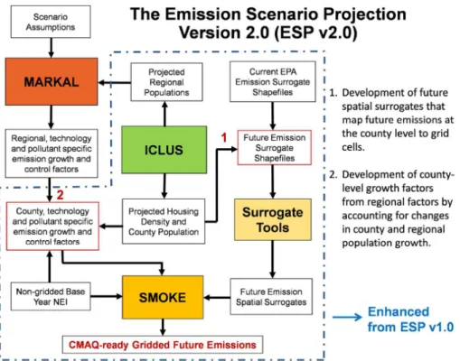
incorporation of ICLUS into ESP v2.0 is depicted in Fig. 1. The two steps associated with spatial allocation of emissions are listed as 1 and 2 in the figure.

The objective of this paper is to describe, demonstrate and evaluate the new spatial allocation features within ESP v2.0. First, the typical approach for spatial allocation in emission processing is described. Next, the new spatial allocation method is presented

5

and evaluated. The method is then applied using an experimental design that isolates the impacts of using projected spatial surrogates and those of mapping regional growth factors to the county level. Conclusions and future plans for ESP v3.0 are presented in the last section.

2 Background

10

In most air quality modeling applications with CMAQ, the SMOKE model is used to transform an emission inventory, such as the NEI, from a textual list of sources and their respective annual emissions to a gridded, temporally allocated, and chemically speciated air quality model-ready binary file. Major steps in the generation of future emissions for an air quality model include the application of multiplicative emission

15

growth and control factors to produce a future-year emission inventory, temporal allo-cation of emissions by season, day and hour, and spatial alloallo-cation of hourly emissions onto a 2-dimensional grid over the modeling domain. A major component of the spatial allocation process is the use of other high-resolution data, such as census block group population or road networks, as surrogates to map county-level emissions to grid cells.

20

Spatial surrogate computation for emission allocation is rarely mentioned in the doc-umentation of air quality modeling studies because it is assumed to be a part of the SMOKE modeling system. In the US, surrogate shapefiles (a standard file format for representing spatial data) are released by the US EPA Emissions Modeling Clearing-house and are used to compute spatial surrogates to be used in SMOKE. Most of the

25

(6)

GMDD

8, 263–300, 2015

L. Ran et al.

Title Page

Tables Figures

◭ ◮

Back Close

Full Screen / Esc

Discussion

P

a

per

|

Discussion

P

a

per

|

Discussion

P

a

per

|

Discussion

P

a

per

|

(such as building square footage and agricultural areas) that were generated around that time period. Note that the spatial surrogate shapefiles were subsequently updated in the 2011 EPA modeling platform (US EPA, 2011; US EPA, 2014).

The surrogate shapefiles are processed to create gridded surrogates using the Sur-rogate Tools software package (Ran, 2014), a part of the Spatial Allocator (SA) system

5

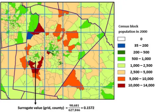
(UNC, 2014). Figure 2 provides an example of the computation of a population-based spatial surrogate for a 12 km grid cell within Wake County, North Carolina, which in-cludes the state’s capital, Raleigh.

The total population range for each census block group area for Wake County and some adjacent counties (dark purple boundaries) in North Carolina is displayed. The

10

surrogate value for any grid cell (i) and county (j) is computed as:

SurrogateValue(i,j)=PSurrogateWeight(i,j) i

SurrogateWeight(i,j) (1)

Wake County’s total population, found by summing the population of each of its census block groups, was 627 846 in 2000. A population of 98 681 lived within the grid cell indicated by the arrow. The population-based spatial surrogate value for this grid cell

15

and county is calculated as 98 681/627 846, or 0.1572. Thus, 15.72 % of Wake County population-related emissions are allocated to this grid cell.

Spatial surrogate values always range from 0 to 1; 0 indicates that no emissions are allocated to the grid cell (e.g., the grid cell does not intersect the county), and 1 indicates that all the county’s emissions are allocated to the grid cell (e.g., the county

20

is completely located within the grid cell). While the example grid cell lies within just one county, quite often a grid cell can cross multiple county boundaries. When this happens, a weighting method (area for polygons, length for lines, or number of points) is used.

As of April 2014, EPA has 91 different spatial surrogate shapefiles (e.g. population,

25

(7)

GMDD

8, 263–300, 2015

L. Ran et al.

Title Page

Tables Figures

◭ ◮

Back Close

Full Screen / Esc

Discussion

P

a

per

|

Discussion

P

a

per

|

Discussion

P

a

per

|

Discussion

P

a

per

|

each surrogate has to be generated for each modeling grid domain, and air qual-ity modeling often includes multiple nested domains, the Surrogate Tools and their associated quality assurance functions make surrogate computation much easier for preparing emission input to air quality models.

Accurate spatial allocation is particularly important for finer resolution modeling (e.g.

5

12 km or less) when multiple modeling grid cells are located within a county. While most previous CMAQ studies of future air quality have been conducted at relatively coarse resolutions (≥36 km) (Hogrefe et al., 2004; Tagaris et al., 2007; Nolte et al., 2008), finer resolutions are becoming more common with the rapid advancement of computing capabilities (Zhang et al., 2010). Thus, considering landscape changes due

10

to human activities becomes particularly important in emission spatial allocation for high resolution air quality modeling over long time horizons into the future.

3 Method

Spatial allocation in ESP v2.0 involves the two-step process displayed in Fig. 1. For this paper, the method is demonstrated for a 2050 emission scenario, projecting 2005

15

base-year emissions using growth factors from MARKAL. We use ICLUS-produced population and housing density projections that assume county-level population growth in line with the US Census Bureau projections and a land use development pattern that follows historic trends (US EPA, 2009a). The method is applied to the conterminous US (CONUS) study area, excluding Mexico and Canada, with additional analysis

con-20

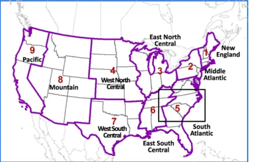
ducted on the Southeast US. The CONUS area, MARKAL emission projection regions, CMAQ 12 km modeling domain, and the Southeast area are depicted in Fig. 3. The grid uses the standard Lambert Conformal Conic Projection, with 299 grid rows and 459 columns andX andY minimums of−2 556 000 and−1 728 000 m, respectively.

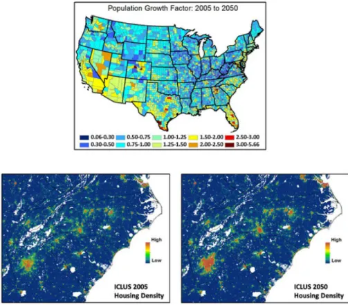
Figure 4 shows county-level population growth factors over the CONUS as well as

25

(8)

rel-GMDD

8, 263–300, 2015

L. Ran et al.

Title Page

Tables Figures

◭ ◮

Back Close

Full Screen / Esc

Discussion

P

a

per

|

Discussion

P

a

per

|

Discussion

P

a

per

|

Discussion

P

a

per

|

atively large cities (e.g. Atlanta, Georgia and Charlotte, North Carolina) and a resulting increase in housing density around those urban areas. In general, county populations increase in most southern and coastal counties, but decrease in northern and inland rural counties.

The approaches for using these ICLUS projections to disaggregate regional emission

5

growth factors and create future-year spatial surrogates are presented below.

3.1 Developing county-level emission growth factors

MARKAL outputs include regional growth factors for energy-related Source Category Codes (SCCs). SMOKE projection packets with growth factors for each species and source category of interest were generated, as described by Loughlin et al. (2011).

10

The six emission source sectors (US EPA, 2011) included in this projection were: 1. Point sources from the Electric Generating Utility (EGU) sector

2. Non-EGU point sources (e.g. airports)

3. Remaining nonpoint sources (area sources not in agriculture and fugitive dust sectors)

15

4. Onroad mobile sources (e.g. light duty vehicles) 5. Nonroad mobile sources (e.g. construction equipment)

6. Mobile emissions from aircraft, locomotives, and commercial marine vessels Though MARKAL-generated regional growth factors capture large-scale emission growth patterns, they do not capture variation in growth from one state to another

20

(9)

GMDD

8, 263–300, 2015

L. Ran et al.

Title Page

Tables Figures

◭ ◮

Back Close

Full Screen / Esc

Discussion

P

a

per

|

Discussion

P

a

per

|

Discussion

P

a

per

|

Discussion

P

a

per

|

LetFp denote the regional population growth factor and fp denote the county-level

population growth factor. The ratio offpoverFpcaptures the relative population growth

rate of a county in comparison to its region (e.g.f_p/Fp=1 means the same growth rate

andfp/Fp>1 means the county population growth is greater than the regional average

growth). The regional emission growth factorFe is adjusted by this ratio in computing

5

the initial county emission growth factorf′

e:

f′

e(r,j, SCC,s)=Fe(r, SCC,s)·

fp(r,j)

Fp(r)

(2)

wherer is the region,j is a county withinr, and s is the species. To ensure that the total regional projected emissions are preserved after applying the county-level growth factors, the projected county emissions are re-normalized as:

10

e2050(r,j, SCC,s)=[f

′

e(r,j, SCC,s)·e2005(r,j, SCC,s)]·Rre(r, SCC,s) (3)

wheree2005ande2050are county-level emissions for 2005 and 2050 andRreis the ratio

of regional emissions computed using regional growth factors to regional emissions derived from county growth factors:

Rre(r, SCC,s)=

Fe(r, SCC,s)·

P j

e2005(r,j, SCC,s)

P j

f′

e(r,j, SCC,s)·e2005(r,j, SCC,s)

(4)

15

The final county emission growth factors (fe) are then computed as:

fe(r,j, SCC,S)=

e2050(r,j, SCC,s)

e₂₀₀₅(r,j, SCC,s) (5) For source categories expected to have emissions changes correlated with population changes, the resulting set offe(r,j, SCC,s) factors are then used to grow the

match-ing county-level emissions into the future. A spreadsheet with example calculations is

20

(10)

GMDD

8, 263–300, 2015

L. Ran et al.

Title Page

Tables Figures

◭ ◮

Back Close

Full Screen / Esc

Discussion

P

a

per

|

Discussion

P

a

per

|

Discussion

P

a

per

|

Discussion

P

a

per

|

Changes in the spatial distribution of some emissions will not necessarily be corre-lated with population shifts, however. For example, we use regional emission growth factors, Fe (r, SCC,s), for electric utilities, large external combustion boilers, and

petroleum refining.

We applied ESP v2.0 to grow the 2005 NEI (US EPA, 2010) inventory to 2050.

Fig-5

ure 5 displays representative county-level emission growth factors. The two plots on the left are the MARKAL regional growth factors for NO_xfrom highway Light Duty Gasoline Vehicles (LDGV) and for SO2from residential stationary source fuel combustion, both

of which would be expected to be correlated with population. The overall regional emis-sion trends are driven by population growth, fuel switching and regulations that limit

10

emissions. The county-level growth factors illustrate the e_ffects of projected county-by-county population changes on these overall trends. County-level emission growth factors, we then generated SMOKE projection packets and used SMOKE to grow the emission inventory to 2050.

3.2 Updating surrogate shapefiles and emission surrogates

15

The next step in spatial allocation is to create surrogate shapefiles using ICLUS-projected population and housing density. Standard EPA population and housing sur-rogate shapefiles are slightly di_fferent from 2005 ICLUS data. To avoid this discrepancy and ensure that surrogate shapefiles are generated consistently for comparison, ICLUS data are used to develop both the 2005 base and the 2050 shapefiles.

20

3.2.1 Surrogate shapefiles

Using ICLUS data, we created four new surrogate shapefiles for both 2005 and 2050. The first shapefile contains census block group polygons with associated population, housing units, urban, and level of development (e.g., no, low or high). The census poly-gon boundaries are based on the EPA 2002 population surrogate shapefiles. For each

25

(11)

GMDD

8, 263–300, 2015

L. Ran et al.

Title Page

Tables Figures

◭ ◮

Back Close

Full Screen / Esc

Discussion

P

a

per

|

Discussion

P

a

per

|

Discussion

P

a

per

|

Discussion

P

a

per

|

using the area weighted method. Then, ICLUS county population is allocated to each census block group within a county according to the fraction of the county’s housing units within that block group. Using ICLUS outputs for 2000, 2005, 2040, and 2050, we computed housing unit changes from 2000 to 2005 and from 2040 to 2050, which are needed for housing unit change surrogate computation for 2005 and 2050. For both

5

2005 and 2050, we classified census block groups as urban if their ICLUS-produced population density per square mile is≥1000. This criterion is partially consistent with

the US Census Bureau’s definition of an urban area, although for simplicity, we did not use the Census Bureau’s requirement of the surrounding area having a total population of 50 000 or more. In addition, census block groups were classified into no, low, or high

10

development areas based on housing density.

Figure 6 shows the change in population and urban surrogate shapefile data over the Southeast region between 2005 and 2050. The figure indicates expansion of urban ar-eas, including Atlanta, Charlotte, Greensboro, and Raleigh. However, some rural arar-eas, particularly in the north and south of this region, display slightly decreasing population

15

densities.

The second surrogate shapefile we generated contains road networks. Though road networks are likely to expand in the future, it is very difficult to project future road networks. We use existing current road surrogate shapefiles with the ICLUS-identified urban areas to classify roads into four categories: rural and urban primary roads and

20

rural and urban secondary roads. These categories are required for surrogate com-putation for mobile emission allocations. The third surrogate shapefile we generated contains rural land classification. We created this shapefile from the EPA 2002 rural land surrogate shapefile using urban and non-urban areas identified in the first shape-file. The last surrogate shapefile we created contains agricultural land classes. This

25

(12)

GMDD

8, 263–300, 2015

L. Ran et al.

Title Page

Tables Figures

◭ ◮

Back Close

Full Screen / Esc

Discussion

P

a

per

|

Discussion

P

a

per

|

Discussion

P

a

per

|

Discussion

P

a

per

|

3.2.2 Surrogates computation

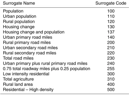
With the ICLUS-based surrogate shapefiles, we computed 2005 and 2050 surrogates using the Surrogate Tools. As noted previously, EPA employs a set of 65 spatial surro-gates to allocate emissions from various source sectors to a gridded modeling domain. The 17 surrogates listed in Table 1 were computed using the four ICLUS-based

shape-5

files. We assumed that the other 48 surrogates remain unchanged from current EPA surrogates.

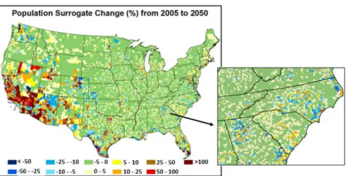
The percentage change of ICLUS population-based surrogates from 2005 to 2050 is shown in Fig. 7. As expected, population-based surrogate changes on the 12 km grid follow the trends shown in Fig. 4. Since surrogates for the grid cells intersecting

10

a county necessarily sum to 1, large surrogate increases (red colors) in some grid cells are often accompanied by large decreases (blue colors) in other grid cells within the same county. Large percentage changes are particularly obvious in sparsely populated areas, such as parts of California, Nevada, Arizona, New Mexico, Texas, and Florida. The mean change of population-based surrogates from 2005 to 2050 is 6.23 %,

al-15

though a standard deviation of 46.96 % indicates a wide range across the grid cells.

4 Application

We applied ESP v2.0 to generate 2005 and 2050 CMAQ-ready gridded emission files. Only the six sectors listed above from the 2005 NEI were used in the 2050 projection. Emissions from any SCCs not included in the projection packets were held constant

20

from 2005. We used the Emission Modeling Framework (Houyoux et al., 2006) to con-duct SMOKE modeling tasks.

Next, two additional 2050 inventories were created, one using the regional growth factors from MARKAL and one using the surrogates based upon 2005 ICLUS results. The four resulting gridded inventories that were developed are listed in Table 2.

(13)

GMDD

8, 263–300, 2015

L. Ran et al.

Title Page

Tables Figures

◭ ◮

Back Close

Full Screen / Esc

Discussion

P

a

per

|

Discussion

P

a

per

|

Discussion

P

a

per

|

Discussion

P

a

per

|

Futurerepresents the result of the full ESP v2.0 projection method. Comparing Fu-turewith Base thus reveals the projected changes in both magnitude and location of emissions over the 45 year period. ComparingFuturewithFuture-RegGF isolates the effects of disaggregating regional growth factors to the county level. Similarly, compar-ing Future with Future-05Surr identifies spatial changes resulting from updating the

5

future spatial surrogates.

The Fractional Difference (FD) metric is used to evaluate grid-level differences among the inventories. For a model grid cell (i) and species (s), the FD is calculated as:

Fractional Difference (FD)=2· _e

A(i,s)−eB(i,s)

e_A(i,s)+e_B(i,s)

·100 (6)

10

whereeA(i,s) andeB (i,s) are the emissions of speciess in grid celli for the gridded

inventories,A and B, that are being compared. FD is generally called fractional bias when it is used to evaluate errors of modeling results against observations (e.g. Morris et al., 2006). FD is a symmetric metric ranging from −200 % to ₊200 %. A value of

67 % for FD represents that eA is larger than eB by a factor of two, while an FD of 15

0 means that values are the same. The mean and standard deviation of FD values across groups of grid cells provide information about the magnitude and variability of differences between two gridded inventories. Other statistical metrics can be used to evaluate differences from one gridded inventory to another. Several such metrics are described and applied in the Supplement to this paper.

20

4.1 Base and future emission di_fferences

Figure 8 shows FDs between annual emissions in theBaseandFuturefor each of the six projected pollutant species. These plots reflect the combined effects of population growth and migration, economic growth and transformation, fuel switching, technologi-cal improvements, land use change, and various regulations limiting emissions

(Lough-25

(14)

GMDD

8, 263–300, 2015

L. Ran et al.

Title Page

Tables Figures

◭ ◮

Back Close

Full Screen / Esc

Discussion

P

a

per

|

Discussion

P

a

per

|

Discussion

P

a

per

|

Discussion

P

a

per

|

in modeled NO_x, SO₂, CO, VOC, PM_2.5 and PM₁₀. Grids with emission increases for these six species are mainly located in areas projected to have high population growth (e.g. Los Angeles and Atlanta). Among the six species, NOxand SO2show reductions

of more than a factor of 2 in many areas because of control requirements on electricity production, transportation, and many industrial sources. Emissions of CO, VOC, PM2.5

5

and PM10also fall across most of the domain.

4.2 Region-to-county growth disaggregation

We evaluate the effect of disaggregating regional growth factors to the county level by examining the differences betweenFuture and Future-RegGF. Grid cell-level FD val-ues are shown in Fig. 9 for the six projected pollutants. The spatial distributions of FD

10

indicates that regional-to-county disaggregation results in increased emissions around urban areas (e.g. Los Angeles, Las Vegas and Dallas in the West and Atlanta in the Southeast) as those areas expand into surrounding counties. Many grid cells at the fringe of large urban areas have FD values exceeding 30 %, indicating a large relative increase in emissions as a result of using county-level growth factors. Large

reduc-15

tions in emissions, indicated by FD values ≤ −20 %, are particularly obvious in rural areas in the West and South regions. County-level growth factors have high impacts on emission allocations in the regions of the West and South, particularly for SO₂.

Another way to analyze FD results is to calculate mean FD (MFD) values across grid cells with common characteristics. For example, in Fig. 10, we provide mean FDs for

20

each pollutant over grid cells that are in the same population density range.

For areas with greater density, the trend is that emission differences become in-creasingly positive, reflecting that the ICLUS population algorithm typically results in migration of people to more dense areas. However, as described above, the ICLUS pre-dicts continued urban sprawl such that the positive MFD in the urban cores (population

25

density≤200 k grid−1, about 1400 km−2) is slightly less than in the more moderately

(15)

emis-GMDD

8, 263–300, 2015

L. Ran et al.

Title Page

Tables Figures

◭ ◮

Back Close

Full Screen / Esc

Discussion

P

a

per

|

Discussion

P

a

per

|

Discussion

P

a

per

|

Discussion

P

a

per

|

sion changes by region without using the county growth allocation method significantly

underestimatesthe future emissions in the more populated areas.

4.3 Updating emission surrogates

We evaluate the effects of adjusting future surrogates by comparingFutureand Future-05Surr. The two gridded emission files were generated from the same 2050

county-5

level emission growth factors, but using ICLUS-derived surrogates for 2050 and 2005, respectively. Thus, emission differences are introduced only from different spatial sur-rogates. Figure 11 presents the resulting FD values for the six projected pollutants.

In Fig. 11, it is apparent that large increases (FD>20 %) often occur in the grid cells surrounding large cities. Further, FD% increases are particularly obvious in the West

10

and Southwest regions, where urban expansion moves into previously low density grid cells. The counties in these regions tend to be large; thus, changes in spatial surrogates affect a larger number of grid cells. In contrast, changes in gridded emissions tend to be less pronounced in areas with small counties that are closer in size to the 12 km×12 km

grid cells. Updating the spatial surrogates has a small or negligible impact in rural areas

15

with limited urbanization. Among the six compared species, SO2has the least changes.

SO₂ emissions from mobile sources are reduced considerably by regulations limiting sulfur content in fuels. Most of the remaining SO₂emissions originate from electricity production and industrial sources. In the ESP v2.0 method, we do not adjust the spatial distribution of electric utilities or other industries, assuming that they are not correlated

20

with population. In contrast, incorporating the 2050 surrogates has particularly high impacts on CO and VOC. Major sources for these pollutants are the transportation, residential and commercial sectors, all of which are linked to population- and land-use base surrogates.

Figure 12 also provides an indication of how updating surrogates affects emissions

25

(16)

GMDD

8, 263–300, 2015

L. Ran et al.

Title Page

Tables Figures

◭ ◮

Back Close

Full Screen / Esc

Discussion

P

a

per

|

Discussion

P

a

per

|

Discussion

P

a

per

|

Discussion

P

a

per

|

in the densest areas. Conversely, there is an increase in emissions from categories ranging in density from 5 to 80 k per cell.

Thus, emissions using 2050 surrogates allocate more emissions to the suburban areas as they densify, while emissions allocated to the high density urban core grid cells are reduced. This does not mean that populations in cities are projected to

de-5

cline, but rather that the projected urban emissions are partially re-distributed to the fringe areas since county emission totals are the same for both scenarios. This anal-ysis demonstrates that the common practice of projecting future emissions without projecting future surrogates can lead to over-prediction of urban core emissions and under-prediction of suburban/exurban emissions.

10

5 Conclusions

Gridded emission data are key inputs to air quality models. Pollutant growth factors play a dominant role in determining regional emission and air quality patterns (Tao et al., 2007; Avise et al., 2009). It is commonplace in such applications to apply these growth factors such that emissions are grown in place. In this paper, we demonstrate

15

that the region-to-county growth factor disaggregation and county-to-grid allocation ap-proaches included in ESP v2.0 yield a different spatial pattern of emissions. For a given population and land use change scenario, the region-to-county growth disaggregation enables the distinction of different growth levels among counties, and updating spatial surrogates provides a more realistic mapping of emissions to grid cells.

20

Conversely, growing residential emissions in place and applying current spatial surro-gates to future-year emissions may result in an overprediction of urban core emissions and under-prediction of suburban emissions. Thus, ignoring these shifts may overstate future improvements in human exposure and health risk due to air pollution mitigation as more dense urban cores yield greater opportunities for human exposures (e.g. Post

25

(17)

GMDD

8, 263–300, 2015

L. Ran et al.

Title Page

Tables Figures

◭ ◮

Back Close

Full Screen / Esc

Discussion

P

a

per

|

Discussion

P

a

per

|

Discussion

P

a

per

|

Discussion

P

a

per

|

There are many uncertainties in future air quality studies associated with emissions, climate, and changes of landscape. Improving emission allocation in SMOKE will help reduce uncertainties in outcomes (e.g. O3and PM2.5concentrations and climate

forc-ing from gases and aerosols) from regional climate and air quality modelforc-ing systems such as the coupled WRF/CMAQ (Wong et al., 2012) and help improve confidence

5

in making air quality policies related to human health and the environment. Another important aspect of the approaches presented here is that they could be applied to examine alternative development scenarios. For example, a smart growth scenario would project greater growth factors in cities and less in suburban/exurban areas than the business as usual scenario on which ICLUS was based. Furthermore, within the

10

larger ESP v2.0 framework, emissions and resulting impacts could be examined for wide ranging scenarios that differ in assumptions about population growth and migra-tion, economic growth and transformamigra-tion, technology change, land use change, and various energy, environmental and land use policies.

Work on the ESP method continues, and a v3.0 is under development. Planned

15

improvements include enhancing the ability to explore economic growth and transfor-mation assumptions and also adding the ability to update temporal profiles for various emission sources. An example of why adjusted temporal profiles could be important is evident when examining the use of natural gas for electricity production. Historically, natural gas has been used within combustion turbines to meet summer afternoon

elec-20

tricity demands associated with air conditioning. With expanded access to natural gas resources, however, electric utilities are incrementally shifting gas to baseload elec-tricity production. Thus, the temporal profile is changing both seasonally and hourly. We plan to explore how to account for these dynamics and to examine their impact on emissions and air quality.

25

(18)

GMDD

8, 263–300, 2015

L. Ran et al.

Title Page

Tables Figures

◭ ◮

Back Close

Full Screen / Esc

Discussion

P

a

per

|

Discussion

P

a

per

|

Discussion

P

a

per

|

Discussion

P

a

per

|

Vuuren et al., 2012). The RCP scenarios are the successors to the IPCC’s SRES sce-narios (IPCC 2000).

Additional updates may be carried out in future work. For example, the underlying growth factors generated with MARKAL change as the ongoing effort of developing the model and underlying data continue. Similarly, the baseline spatial surrogates used

5

here were developed in 2000. These could be updated to the 2010 surrogate files that are now used within the EPA’s 2011 modeling platform. Furthermore, it would be interesting to compare the 2010 surrogates with the 2010 projected surrogate files developed here.

There are a number of limitations associated with ESP v2.0. For example, while we

10

can explore broad-ranging scenarios, we are not currently able to examine the e_ffect of climate change on wildfires, windblown dust, or biogenics. Climate-related changes to these emissions would need to be evaluated outside of ESP v2.0. Similarly, the method has the limitations of each of its components. The MARKAL energy modeling system, for example, does not account for economic feedbacks associated with changes in

en-15

ergy prices. Despite these limitations, ESP v2.0 represents the state-of-the-art method for projecting multi-decadal US air pollutant emissions.

6 Contributions

Limei Ran was the lead author and the lead in designing, implementing and demon-strating the spatial allocation component of ESP 2.0. Dan Loughlin conceived of the

20

project and was instrumental in developing the spatial allocation method. Further, he provided the emission growth and control factors used to develop the future-year inven-tory. Dongmei Yang, Zach Adelman and B.H. Baek assisted with the development and implementation of the method, including applications of the various emissions model-ing components. Chris Nolte was instrumental in developmodel-ing ESP 1.0 and contributed

25

(19)

GMDD

8, 263–300, 2015

L. Ran et al.

Title Page

Tables Figures

◭ ◮

Back Close

Full Screen / Esc

Discussion

P

a

per

|

Discussion

P

a

per

|

Discussion

P

a

per

|

Discussion

P

a

per

|

Model and data availability

Most of the modeling components that comprise this methodology are publically avail-able. SMOKE and the Spatial Allocator can be downloaded from the Community Mod-eling & Analysis System Center (http://www.cmascenter.org). ICLUS modMod-eling tools and land use projections can be obtained from the US EPA (http://www.epa.gov/ncea/

5

global/iclus/). The MARKAL model is distributed by the Energy Technology Systems Analysis Program of the International Energy Agency (http://www.iea-etsap.org). Exe-cuting MARKAL requires licensing and additional software. Please contact Dan Lough-lin (loughLough-lin.dan@epa.gov) for information about obtaining the US EPA’s MARKAL 9-region database, which allows MARKAL to be applied to the US energy system. The

10

EPA’s database is available upon request at no cost. Regional- and county-level emis-sion growth factors and surrogate shapefiles for 2005 and 2050 are available for down-load in the Supplement.

The Supplement related to this article is available online at doi:10.5194/gmdd-8-263-2015-supplement.

15

Acknowledgements. Much of the effort of developing, implementing and demonstrating the spatial allocation method embodied in ESP 2.0 was funded by the US Environmental Protection Agency Office of Research and Development. Alison Eyth, of the US EPA’s Office of Air Quality Planning and Standards, contributed to a previous implementation of the spatial allocation method. ICLUS-related land use projections were provided by Phil Morefield and 20

Britta Bierwagen of the US EPA’s National Center for Environmental Assessment (NCEA). William Benjey helped develop ESPv1.0 and reviewed this manuscript. Others contributing the emission growth factor projections are current and past members of the Office of Research and Development Energy and Climate Assessment Team, including Carol Lenox, Rebecca Dodder, Ozge Kaplan and William Yelverton.

(20)

GMDD

8, 263–300, 2015

L. Ran et al.

Title Page

Tables Figures

◭ ◮

Back Close

Full Screen / Esc

Discussion

P

a

per

|

Discussion

P

a

per

|

Discussion

P

a

per

|

Discussion

P

a

per

|

Disclaimer.While this work has been reviewed and cleared for publication by the US EPA, the views expressed here are those of the authors and do not necessarily represent the official views or policies of the Agency. Mention of software and organizations does not constitute an endorsement.

References

5

Akhtar, F., Pinder, R. Loughlin, D., and Henze, D.: GLIMPSE: a rapid decision frame-work for energy and environmental policy, Environ. Sci. Technol., 47, 12011–12019, doi:10.1021/es402283j, 2013.

Avise, J., Chen, J., Lamb, B., Wiedinmyer, C., Guenther, A., Salathé, E., and Mass, C.: Attri-bution of projected changes in summertime US ozone and PM_2.5 concentrations to global 10

changes, Atmos. Chem. Phys., 9, 1111–1124, doi:10.5194/acp-9-1111-2009, 2009.

Avise, J., Gonzalez-Abraham, R., Chung, S. H. Chen, J., Lamb, B., Salathé, E. P., Zhang, Y., Nolte, C. G., Loughlin, D. H., Guenther, A., Wiedinmyer, C., and Duhl, T.: Evaluating the effects of climate change on summertime ozone using a relative response factor approach for policymakers, J. Air Waste Manage., 62, 1061–1074, 2012.

15

Bierwagen, B. G., Theobald, D. M., Pyke, C. R., Choate, A., Groth, P., Thomas, J. V., and More-field, P.: National housing and impervious surface scenarios for integrated climate impact assessments, P. Natl. Acad. Sci. USA, 107, 20887–20892, 2010.

Byun, D. and Schere, K.: Review of the governing equations, computational algorithms, and other components of the Models-3 Community Multiscale Air Quality (CMAQ) modeling sys-20

tem, Appl. Mech. Rev., 59, 51–77, doi:10.1115/1.2128636, 2006.

Fishbone, L. G. and Abilock, H.: MARKAL: a linear programming model for energy-systems analysis: technical description of the BNL version, Journal of Energy Research, 5, 353–375, 1981.

Hogrefe, C., Lynn, B., Civerolo, K., Ku, K.-Y., Rosenthal, J., Rosenzweig, C., Goldberg, R., 25

(21)

GMDD

8, 263–300, 2015

L. Ran et al.

Title Page

Tables Figures

◭ ◮

Back Close

Full Screen / Esc

Discussion

P

a

per

|

Discussion

P

a

per

|

Discussion

P

a

per

|

Discussion

P

a

per

|

Houyoux, M. R., Vukovich, J. M., Coats, C. J., Wheeler, N. J., and Kasibhatla, P. S.: Emis-sion inventory development and processing for the Seasonal Model for Regional Air Quality (SMRAQ) project, J. Geophys. Res.-Atmos., 105, 9079–9090, 2000.

Houyoux, M. R., Strum, M., Mason, R., and Eyth, A.: Data management using the emissions modeling framework, in: Proceedings of the Fifteenth International Emission Inventory Con-5

ference, 2006.

IPCC 2000, Intergovernmental Panel on Climate Change (IPCC): Special Report on Emissions Scenarios, edited by: Nakicenovic, N. and Swart, R., Cambridge Univ. Press, New York, 612 pp., 2000.

Loughlin, D. H., Benjey, W. G., and Nolte, C. G.: ESP v1.0: methodology for exploring emis-10

sion impacts of future scenarios in the United States, Geosci. Model Dev., 4, 287–297, doi:10.5194/gmd-4-287-2011, 2011.

Loulou, R., Goldstein, G., and Noble, K.: Documentation for the MARKAL family of models, available at: hhttp://www.iea-etsap.org/ (last access: December 2014), 389 pp., 2004. Morris, R. E., Koo, B., Guenther, A., Yarwood, G., McNally, D., Tesche, T. W., and Brewer, P.: 15

Model sensitivity evaluation for organic carbon using two multi-pollutant air quality models that simulate regional haze in the southeastern United States, Atmos. Environ., 40, 4960– 4972, 2006.

Nolte, C. G., Gilliland, A. B., Hogrefe, C., and Mickley, L. J.: Linking global to regional models to assess future climate impacts on surface ozone levels in the United States, J. Geophys. 20

Res.-Atmos., 113, D14307, doi:10.1029/2007JD008497, 2008.

Post, E. S., Grambsch, A., Weaver, C., Morefield, P., Huang, J., Leung, L.-Y., Nolte, C. G., Adams, P., Liang, X.-Z., Zhu, J.-H., and Mahoney, H.: Variation in estimated ozone-related health impacts of climate change due to modeling choices and assumptions, Environ. Health Persp., 120, 1559–1564, 2012.

25

Ran, L. R.: Emissions Modeling Framework Surrogate Tool: User’s Guide, the Community Mod-eling and System Analysis at the University of North Carolina, Chapel Hill, available at: https://www.cmascenter.org/sa-tools/documentation/4.2/html (last access: October 2014), 33 pp., 2014.

Silva, R. A., West, J. J., Zhang, Y., Anenberg, S. C., Lamarque, J.-F., Shindell, D. T., Collins, W. 30

(22)

GMDD

8, 263–300, 2015

L. Ran et al.

Title Page

Tables Figures

◭ ◮

Back Close

Full Screen / Esc

Discussion

P

a

per

|

Discussion

P

a

per

|

Discussion

P

a

per

|

Discussion

P

a

per

|

S., Strode, S., Szopa, S., and Zeng, G.: Global premature mortality due to anthropogenic out-door air pollution and the contribution of past climate change, Environ. Res. Lett., 8, 034005, doi:10.1088/1748-9326/8/3/034005, 2013.

Tagaris, E., Manomaiphiboon, K., Liao, K. J., Leung, L. R., Woo, J. H., He, S., and Rus-sell, A. G.: Impacts of global climate change and emissions on regional ozone and fine 5

particulate matter concentrations over the United States, J. Geophys. Res., 112, D14312, doi:10.1029/2006JD008262, 2007.

Tao, Z., Williams, A., Huang, H.-C., Caughey, M., and Liang, X.-Z.: Sensitivity of US sur-face ozone to future emissions and climate changes, Geophys. Res. Lett., 34, L08811, doi:10.1029/2007GL029455, 2007.

10

Theobald, D. M.: Landscape patterns of exurban growth in the USA from 1980 to 2020, Ecol. Soc., 10, 32, available at: http://www.ecologyandsociety.org/vol10/iss1/art32/ (last access: January 2015), 2005.

UNC: Spatial Allocator Version 4.2, the Community Modeling and System Analysis at the Uni-versity of North Carolina, Chapel Hill, available at: http://www.cmascenter.org/sa-tools/ (last 15

access: October 2014), 2014.

US EIA: Annual Energy Outlook 2006 with Projections to 2030, No: DOE/EIA-0383(2010), US Energy Information Administration, Washington, DC, available at: http://www.eia.gov/oiaf/ archive/aeo06/ (last access: May 2004), 2006.

US EIA: Annual Energy Outlook 2010 with Projections to 2035, No: DOE/EIA-0383, US Energy 20

Information Administration, Washington, DC, available at: http://www.eia.gov/oiaf/archive/ aeo10/ (last access: May 2004), 2010.

US EPA: Land-Use Scenarios: National-Scale Housing-Density Scenarios Consistent with Cli-mate Change Storylines, an interim report of the US EPA Global Change Research Program, EPA/600/R-08/076F, National Center for Environmental Assessment, Washington, DC, avail-25

able at: http://cfpub.epa.gov/ncea/global/recordisplay.cfm?deid=203458 (last access: Au-gust 2013), 2009a.

US EPA: Assessment of the Impacts of Global Change on Regional US Air Quality: a Synthe-sis of Climate Change Impacts on Ground-Level Ozone, an interim report of the US EPA Global Change Research Program, EPA/600/R-07/094F, National Center for Environmental 30

(23)

GMDD

8, 263–300, 2015

L. Ran et al.

Title Page

Tables Figures

◭ ◮

Back Close

Full Screen / Esc

Discussion

P

a

per

|

Discussion

P

a

per

|

Discussion

P

a

per

|

Discussion

P

a

per

|

US EPA: 2005 National Emissions Inventory Data and Documentation, US EPA, Washing-ton, DC, available at: http://www.epa.gov/ttn/chief/net/2005inventory.html (last access: Au-gust 2013), 2010.

US EPA: Emissions Inventory Final Rule Technical Support Document (TSD), US EPA, Office of Air and Radiation, Office of Air Quality Planning and Standards, Research Triangle Park, 5

NC, available at: http://www.epa.gov/airtransport/pdfs/EmissionsInventory.pdf (last access: September 2013), 112 pp., 2011.

US EPA: Emissions Modeling Clearinghouse – Spatial Allocation, available at: http://www.epa. gov/ttn/chief/emch/spatial/ (last access: April 2014), 2014a.

US EPA: DRAFT Technical Support Document: Preparation of Emission Inventories for the Ver-10

sion 6.0, 2011 Emission Modeling Platform, US Environmental Protection Agency, Office of Air and Radiation, available at: http://www.epa.gov/ttn/chief/emch/2011v6/outreach/2011v6_ 2018base_EmisMod_TSD_26feb2014.pdf (last access: August 2014), 2014b.

Van Vuuren, D. P., Edmonds, J., Kainuma, M., Riahi, K., Thomson, A., Hibbard, K., Hurtt, G. C., Kram, T., Krey, Vv., Lamarque, J.-F., Masui, T., Meinshausen, M., Nakicenovic, N., Smith, 15

S. J., and Rose, S. K.: The representative concentration pathways: an overview, Climatic Change, 109, 5–31, 2011.

Van Vuuren, D. P., Riahi, K., Moss, R., Edmonds, J., Thomson, A., Nakicenovic, N., Kram, T., Berkhout, F., Swart, Rob, Janetos, A., Rose, S. K., and Arnell, N.: A proposal for a new scenario framework to support research and assessment in different climate research com-20

munities, Global Environ. Chang., 22, 21–35, 2012.

Weaver, C. P., Liang, X.-Z., Adams, P. J., Amar, P., Avise, J., Caughey, M., Chen, J., Cohen, R. C., Cooter, E., Dawson, J. P., Gilliam, R., Gilliland, A., Goldstein, A. H., Grambsch, A., Grano, D., Guenther, A., Gustafson, W. I., Harley, R. A., He, S., Hemming, B., Hogrefe, C., Huang, H.-C., Hunt, S. W., Jacob, D. J., Kinney, P. L., Kunkel, K., Lamarque, J.-F., Lamb, B., Larkin, N. 25

K., Leung, L. R., Liao, K.-J., Lin, J.-T., Lynn, B. H., Manomaiphiboon, K., Mass, C., McKenzie, D., Mickley, L. J., O’Neill, S. M., Nolte, C., Pandis, S. N., Racherla, P. N., Rosenzweig, C., Russell, A. G., Salathé, E., Steiner, A. L., Tagaris, E., Tao, Z., Tonse, S., Wiedinmyer, C., Williams, A., Winner, D. A., Woo, J.-H., Wu, S., and Wuebbles, D. J.: A preliminary synthesis of modeled climate change impacts on US regional ozone concentrations, B. Am. Meteorol. 30

(24)

GMDD

8, 263–300, 2015

L. Ran et al.

Title Page

Tables Figures

◭ ◮

Back Close

Full Screen / Esc

Discussion

P

a

per

|

Discussion

P

a

per

|

Discussion

P

a

per

|

Discussion

P

a

per

|

West, J. J., Smith, S. J., Silva, R. A., Naik, V., Zhang, Y., Adelman, Z., Fry, M. M., Anenberg, S., Horowitz, L.-W., and Lamarque, J.-F.: Co-benefits of mitigating global greenhouse gas emis-sions for future air quality and human health, Nature Climate Change, 3, 885–889, 2013. Wong, D. C., Pleim, J., Mathur, R., Binkowski, F., Otte, T., Gilliam, R., Pouliot, G., Xiu, A.,

Young, J. O., and Kang, D.: WRF-CMAQ two-way coupled system with aerosol feed-5

back: software development and preliminary results, Geosci. Model Dev., 5, 299–312, doi:10.5194/gmd-5-299-2012, 2012.

Woo, J. H., He, S., Tagaris, E., Liao, K. J., Manomaiphiboon, K., Amar, P., and Russell, A. G.: Development of North American emission inventories for air quality modeling under climate change, J. Air Waste Manage., 58, 1483–1494, 2008.

10

(25)

GMDD

8, 263–300, 2015

L. Ran et al.

Title Page

Tables Figures

◭ ◮

Back Close

Full Screen / Esc

Discussion

P

a

per

|

Discussion

P

a

per

|

Discussion

P

a

per

|

Discussion

P

a

per

|

Table 1.ICLUS-based surrogates generated for 2005 and 2050.

Surrogate Name Surrogate Code

Population 100

Urban population 110

Rural population 120

Housing change 130

Housing change and population 137

Urban primary road miles 140

Rural primary road miles 200

Urban secondary road miles 210

Rural secondary road miles 220

Total road miles 230

Urban primary plus rural primary road miles 240 0.75 total roadway miles plus 0.25 population 255

Low intensity residential 300

Total agriculture 310

Rural land area 400

(26)

GMDD

8, 263–300, 2015

L. Ran et al.

Title Page

Tables Figures

◭ ◮

Back Close

Full Screen / Esc

Discussion

P

a

per

|

Discussion

P

a

per

|

Discussion

P

a

per

|

Discussion

P

a

per

|

Table 2.Standard and sensitivity runs for ESP v2.0 demonstration and evaluation.

Inventory ID Inventory Year ICLUS Surrogates Growth Factors

Base 2005 2005 N/A

Future 2050 2050 County

Future05Surr 2050 2005 County

(27)

GMDD

8, 263–300, 2015

L. Ran et al.

Title Page

Tables Figures

◭ ◮

Back Close

Full Screen / Esc

Discussion

P

a

per

|

Discussion

P

a

per

|

Discussion

P

a

per

|

Discussion

P

a

per

|

(28)

GMDD

8, 263–300, 2015

L. Ran et al.

Title Page

Tables Figures

◭ ◮

Back Close

Full Screen / Esc

Discussion

P

a

per

|

Discussion

P

a

per

|

Discussion

P

a

per

|

Discussion

P

a

per

|

(29)

GMDD

8, 263–300, 2015

L. Ran et al.

Title Page

Tables Figures

◭ ◮

Back Close

Full Screen / Esc

Discussion

P

a

per

|

Discussion

P

a

per

|

Discussion

P

a

per

|

Discussion

P

a

per

|

(30)

GMDD

8, 263–300, 2015

L. Ran et al.

Title Page

Tables Figures

◭ ◮

Back Close

Full Screen / Esc

Discussion

P

a

per

|

Discussion

P

a

per

|

Discussion

P

a

per

|

Discussion

P

a

per

|

(31)

GMDD

8, 263–300, 2015

L. Ran et al.

Title Page

Tables Figures

◭ ◮

Back Close

Full Screen / Esc

Discussion

P

a

per

|

Discussion

P

a

per

|

Discussion

P

a

per

|

Discussion

P

a

per

|

(32)

GMDD

8, 263–300, 2015

L. Ran et al.

Title Page

Tables Figures

◭ ◮

Back Close

Full Screen / Esc

Discussion

P

a

per

|

Discussion

P

a

per

|

Discussion

P

a

per

|

Discussion

P

a

per

|

(33)

GMDD

8, 263–300, 2015

L. Ran et al.

Title Page

Tables Figures

◭ ◮

Back Close

Full Screen / Esc

Discussion

P

a

per

|

Discussion

P

a

per

|

Discussion

P

a

per

|

Discussion

P

a

per

|

(34)

GMDD

8, 263–300, 2015

L. Ran et al.

Title Page

Tables Figures

◭ ◮

Back Close

Full Screen / Esc

Discussion

P

a

per

|

Discussion

P

a

per

|

Discussion

P

a

per

|

Discussion

P

a

per

|

(35)

GMDD

8, 263–300, 2015

L. Ran et al.

Title Page

Tables Figures

◭ ◮

Back Close

Full Screen / Esc

Discussion

P

a

per

|

Discussion

P

a

per

|

Discussion

P

a

per

|

Discussion

P

a

per

|

(36)

GMDD

8, 263–300, 2015

L. Ran et al.

Title Page

Tables Figures

◭ ◮

Back Close

Full Screen / Esc

Discussion

P

a

per

|

Discussion

P

a

per

|

Discussion

P

a

per

|

Discussion

P

a

per

|

(37)

GMDD

8, 263–300, 2015

L. Ran et al.

Title Page

Tables Figures

◭ ◮

Back Close

Full Screen / Esc

Discussion

P

a

per

|

Discussion

P

a

per

|

Discussion

P

a

per

|

Discussion

P

a

per

|

(38)

GMDD

8, 263–300, 2015

L. Ran et al.

Title Page

Tables Figures

◭ ◮

Back Close

Full Screen / Esc

Discussion

P

a

per

|

Discussion

P

a

per

|

Discussion

P

a

per

|

Discussion

P

a

per

|