www.atmos-chem-phys.net/12/8993/2012/ doi:10.5194/acp-12-8993-2012
© Author(s) 2012. CC Attribution 3.0 License.
Chemistry
and Physics
Estimation of mercury emissions from forest fires, lakes, regional
and local sources using measurements in Milwaukee and
an inverse method
B. de Foy1, C. Wiedinmyer2, and J. J. Schauer3
1Department of Earth and Atmospheric Sciences, Saint Louis University, MO, USA 2National Center of Atmospheric Research, Boulder, CO, USA
3Civil and Environmental Engineering, University of Wisconsin – Madison, WI, USA Correspondence to:B. de Foy (bdefoy@slu.edu)
Received: 19 April 2012 – Published in Atmos. Chem. Phys. Discuss.: 23 May 2012 Revised: 17 September 2012 – Accepted: 18 September 2012 – Published: 2 October 2012
Abstract.Gaseous elemental mercury is a global pollutant that can lead to serious health concerns via deposition to the biosphere and bio-accumulation in the food chain. Hourly measurements between June 2004 and May 2005 in an ur-ban site (Milwaukee, WI) show elevated levels of mercury in the atmosphere with numerous short-lived peaks as well as longer-lived episodes. The measurements are analyzed with an inverse model to obtain information about mercury emissions. The model is based on high resolution meteoro-logical simulations (WRF), hourly back-trajectories (WRF-FLEXPART) and a chemical transport model (CAMx). The hybrid formulation combining back-trajectories and Eulerian simulations is used to identify potential source regions as well as the impacts of forest fires and lake surface emissions. Uncertainty bounds are estimated using a bootstrap method on the inversions. Comparison with the US Environmental Protection Agency’s National Emission Inventory (NEI) and Toxic Release Inventory (TRI) shows that emissions from coal-fired power plants are properly characterized, but emis-sions from local urban sources, waste incineration and metal processing could be significantly under-estimated. Emissions from the lake surface and from forest fires were found to have significant impacts on mercury levels in Milwaukee, and to be underestimated by a factor of two or more.
1 Introduction
Elemental mercury emitted to the atmosphere has a life-time ranging from one half to two years (Lindberg et al., 2007; Schroeder and Munthe, 1998) making it a global pol-lutant. There is extensive cycling between different stocks of mercury (atmosphere, oceans, lithosphere) which further adds to the time scale and complexity of mercury concentra-tions in the atmosphere (Selin, 2009). Mercury reacts to form methylmercury which is highly toxic and bioaccumulates in the food chain leading to global health concerns (Mergler et al., 2007).
Before 1970, the main anthropogenic sources were thought to be chloralkali plants, but dominant sources now are coal-fired power plants, waste incineration and metal pro-cessing (Schroeder and Munthe, 1998). While some point sources are well characterized with uncertainties within 30 % for power plants for example, sources such as waste incin-eration and various industrial processes have uncertainties of a factor of five or more (Lindberg et al., 2007). Pirrone et al. (2010) estimate current global natural sources to be 5200 t yr−1 and anthropogenic emissions to be 2300 t yr−1.
Half of the naturally emitted mercury is from the oceans, 13 % from forest fires and most of the balance from vege-tation.
mercury from terrestrial and aquatic surfaces. Although global emissions of mercury are believed to be increasing, the global average atmospheric concentration of mercury has decreased since the mid-1990s (Slemr et al., 2011). The cause of the discrepancy is unknown. One hypothesis rele-vant to this study is that there have been significant shifts in the re-emissions of mercury due to climate change, ocean acidification, and excess input of nutrients to terrestrial and aquatic ecosystems (Slemr et al., 2011). As regulatory con-trols on mercury emissions impact fresh mercury emissions and as re-emissions rates are potentially changing, there is an increased need to develop tools to quantify the emissions of mercury from air pollution sources and to quantify and track re-emissions of legacy mercury in the environment.
Emissions modeling is required to simulate natural sources of mercury, which, as noted above, are thought to account for approximately two thirds of total emissions. Lin et al. (2005) developed an emissions processor using a meteoro-logical model to estimate continental US vegetation emis-sions between 28 and 127 t yr−1and corresponding impacts of up to 0.2 ng m−3on average gaseous elemental mercury concentrations. Bash et al. (2004) developed a surface emis-sion model for vegetation, soils and water sources yield-ing flux estimates in the range of 1.5 to 4.5 ng m−2h−1 for the three source types, in agreement with previously pub-lished estimates. However, estimates using measurements from a relaxed eddy accumuluation system yielded consid-erably higher estimates (22±33 ng m−2h−1) above a for-est canopy (Bash and Miller, 2008). Further developing the emissions model, Bash (2010) estimate the extensive recy-cling of mercury that takes place between the atmosphere, terrestrial and surface water stocks. Similar emissions esti-mates were found by Gbor et al. (2006), who show that in-cluding natural emissions improves model performance for total gaseous mercury. Using these estimates, Gbor et al. (2007) find that their domain, which includes the Eastern US and Southeastern Canada, is a net source of mercury to the atmosphere.
Comparison of measurements in coastal and rural sites found impacts of surface water emissions of mercury on at-mospheric concentrations (Engle et al., 2010). Ocean emis-sions were also found to impact mercury levels in New Hampshire (Sigler et al., 2009). A modeling study found that although globally the ocean is a sink of mercury, the North Atlantic is a net source with 40 % of the emissions coming from subsurface water. These are potentially due to historical anthropogenic sources (Soerensen et al., 2010).
Chemical transport modeling of mercury has been devel-oped mainly to estimate deposition rates and is subject to a combination of large uncertainties in emissions as well as in chemical reactions (Lin and Tao, 2003; Roustan and Bocquet, 2006; Seigneur et al., 2004; Bullock et al., 2008). Yarwood et al. (2003) used Eulerian modeling to evaluate mercury deposition in Wisconsin and found that there was a significant need to improve model boundary conditions and
the treatment of wet deposition. A further study by Seigneur (2007) found that anthropogenic North American sources likely contributed between 15 and 40 % of mercury deposi-tion in Wisconsin, with less than 10 % contribudeposi-tion from US coal-fired power plants.
Sprovieri et al. (2010) review worldwide measurements of atmospheric mercury and note that there are significant un-knowns in the spatial distribution of mercury deposition in relation to sources. For example, there can be low values of deposition close to large power plants in Pennsylvania and Ohio, and high values in Florida. Furthermore, values in ur-ban locations can be a factor of two or greater than at rural sites. Murray and Holmes (2004) had already noted differ-ences by up to a factor of two in different emissions inven-tories for the Great Lakes and identified that some industrial sources have particularly uncertain emissions. Nevertheless, Cohen et al. (2004) found that estimated deposition rates to the Great Lakes were consistent with measurements. Using a model for particle trajectories, they show that sources up to 2000 km away can have significant impacts and that coal combustion is the largest contributor although sources such as incineration and metal processing are significant too.
There have been several measurement studies in Wiscon-sin aimed at identifying sources of mercury. Manolopoulos et al. (2007a) made year long measurements at a rural site and found significant impacts from a local coal-fired power plant on reactive gaseous mercury, but not elemental mer-cury. They recommend the use of receptor-based monitoring to account for small-scale sources and processes that cannot be represented in large-scale Eulerian models. Kolker et al. (2010) perform a separate study with three rural measure-ment sites. They find that the site closest to the coal-fired power plant does not always experience the highest mercury levels and suggest three possible reasons: the presence of a chlor-alkali facility, the plume height, and/or the formation of reactive gaseous mercury in the plume. They do find that elevated levels are due to wind transport from the south, but cannot differentiate between local sources or the more dis-tant Chicago area which is in the same direction. Rutter et al. (2008) compare measurements from the rural site reported in Manolopoulos et al. (2007a) and from an urban site in Milwaukee. They report on a significant urban excess in ele-mental gaseous mercury and suggest that point sources could account for a third of the gaseous elemental mercury in Mil-waukee. Further analysis by Engle et al. (2010) includes a comparison of this data with other rural, urban and coastal sites in the US, and further reinforce the suggestion that mer-cury in Milwaukee is significantly impacted by local point sources.
power plants within a 60 km radius. Liu et al. (2010) find that Detroit has an urban excess in mercury concentrations similar to that reported for Milwaukee. Similar findings were reported for Toronto (Cheng et al., 2009) and for a remote site in Western Ontario (Cheng et al., 2012). Other studies have identified alternative sources such as Taconite mining (Han et al., 2005) as well as melting snow and local mobile sources (Huang et al., 2010). In addition to anthropogenic sources, several studies identified the importance of natural sources, including vegetation sources (Wen et al., 2011) and the Atlantic Ocean (Han et al., 2007).
Inverse methods can be used to estimate regional emis-sions from measurements of atmospheric concentrations as reviewed in Manning (2011). This has been widely done using Eulerian grid models and is being increasingly ap-plied with Lagrangian Particle Dispersion Models. For ex-ample, Lauvaux et al. (2008) use backward trajectories to evaluate emissions based on airborne measurements during a field campaign. Stohl et al. (2009) use a Bayesian formu-lation to estimate global and regional sources of long-lived atmospheric trace gases (hydrofluorocarbons and hydrochlo-rofluorocarbons). The sensitivity matrix relating emission sources to atmospheric concentrations is derived using back-trajectories from WRF-FLEXPART. Brioude et al. (2011) use a variant of the method to account for lognormal distri-bution of the measurements and the prior emission estimates for Houston, Texas. A two-step method is used by Roeden-beck et al. (2009) and Rigby et al. (2011). This combines high resolution back-trajectory simulations for local sources with Eulerian simulations for more distant sources. Manning et al. (2011) use a variable grid resolution for the emissions inversion to take into account the reduced model sensitivity for areas far away from the measurement sites. Furthermore, they use an alternative inversion method based on simulated annealing with a cost function that combines a number of different statistical metrics.
In this study, we combine urban measurements from Mil-waukee (Rutter et al., 2008) with meteorological analysis and back-trajectory simulations to identify sources respon-sible for the gaseous elemental mercury concentrations. We develop a method that is a variant of the inversion method described in Stohl et al. (2009) with elements of the two-step approach of Rigby et al. (2011) and the varying resolution method of Manning et al. (2011). This hybrid inverse model is used to evaluate a range of sources of mercury: local, re-gional and distant sources, forest fires and lake surface emis-sions.
We intentionally restrict the study to the transport of gaseous elemental mercury (GEM). This simplifies the in-version method because GEM has an atmospheric lifetime greater than 6 months and so can be treated as a passive tracer. Whereas chemical transformation and deposition are important sources and sinks in the mercury cycle, they do not significantly alter the concentrations of GEM itself on the temporal and spatial scales considered in this study.
In addition to the inverse method, we present a more ba-sic analysis using both wind roses and Concentration Field Analysis (CFA, see Section 2.3) as an independent check on the results. Furthermore, we use a time scale analysis (Sec-tion 4.2) to evaluate the limits in temporal resolu(Sec-tion of the inverse method and thereby improve the emissions estimate of local sources.
2 Methods
2.1 Measurements
Ambient mercury measurements were made at an urban site located north of downtown Milwaukee at 2114◦E. Kenwood Blvd, Milwaukee, WI, USA (43◦06′29′′N, 87◦53′02′′W). The location is 0.5 to 1 mile from Lake Michigan. The sam-pling intake is 1.5 m above the roof of a two story build-ing. The site is on the southern edge of the campus of the University of Wisconsin - Milwaukee. There are some large structures to the north, but the site is otherwise surrounded by a residential neighborhood. Measurements were made from 28 June 2004 to 11 May 2005 (inclusive). A real time in situ ambient mercury analyzer was used from Tekran, Inc., to measure gaseous elemental mercury (GEM), reac-tive gaseous mercury (RGM) and particulate mercury (PHg). In this study we focus on the GEM measurements. Ambient air was pumped into the instrument at a rate of 10 l−1min for 1 h followed by 1 h for analysis of RGM and PHg. GEM was collected onto gold granules over 5 min periods during the hour that RGM and PHg were collected. It was then ther-mally extracted and measured using Cold Vapor Atomic Flu-orescence Spectroscopy (CVAFS). The measurement are de-scribed in greater detail in Rutter et al. (2008) and the refer-ences therein.
For the meteorological analysis, we use Integrated Surface Hourly Data from the National Climatic Data Center which has hourly wind and temperature observations. The near-est site is at General Mitchell International Airport 10 miles south of the measurement site.
2.2 Meteorological simulations
Mesoscale meteorological simulations were performed using the Weather Research and Forecasting Model (WRF) ver-sion 3.3.1 (Skamarock et al., 2005). The boundary and initial conditions were obtained from the North American Regional Reanalysis (Mesinger et al., 2006) which has a horizontal resolution of 32 km. WRF was run with two-way nesting on 3 domains of 27, 9 and 3 km horizontal resolution with 41 vertical levels. Figure 1 shows a map with the three domains. The model set-up is identical to the one described in de Foy et al. (2012).
D1
D2
D3
100° W
90° W 80° W
40° N 50° N
Fig. 1.Map showing the 3 WRF domains (black, blue and green) and the polar grid used for the inverse model (pink) (particle back-trajectories were mapped onto the polar grid for the Residence Time Analysis).
the WSM 3-class simple ice microphysics scheme, the God-dard shortwave scheme and the RRTM longwave scheme. 69 individual simulations were performed each lasting 162 h: the first 42 h were considered spin-up time, and the remain-ing 5 days were used for analysis.
2.3 Lagrangian simulations
Stochastic particle trajectories were calculated with FLEX-PART (Stohl et al., 2005) using WRF-FLEXFLEX-PART (Fast and Easter, 2006; Doran et al., 2008). Back-trajectories were cal-culated for every hour of the campaign by releasing 1000 particles throughout the hour from a randomized height be-tween 0 and 50 m above the ground. We performed tests with a reduced set of 500 particles per hour to confirm that 1000 particles were sufficient and that the results did not depend on the choice of this parameter. This is consistent with sen-sitivity tests by Wen et al. (2011) who use 3000 particles per hour. Particle locations were calculated for 6 days and were saved every hour for analysis. Vertical diffusion coeffi-cients were calculated based on the WRF mixing heights and surface friction velocity. Sub-grid scale terrain effects were turned off and a reflection boundary condition was used at the surface to eliminate deposition effects in the Lagrangian model. This is consistent with the treatment of GEM as a passive tracer.
Residence Time Analysis (RTA, Ashbaugh et al., 1985) was obtained by counting all particle positions every hour on a grid. This yields a gridded field representing the time that the air mass has spent in each cell before arriving at the re-ceptor site. The units of this field are in particle·hours. This can be done for different vertical extents. For the Concentra-tion Field Analysis, we count particles in the entire vertical
column up to the model top. For the inverse model, we count particles in the bottom 1000 m as discussed in Section 2.6.
The RTA can be used for a Concentration Field Analysis (CFA, Seibert et al., 1994) to identify potential source re-gions using concentration measurements at a receptor site, see also (de Foy et al., 2009, 2007). Results will be presented using the GEM concentrations and a grid with 45 km resolu-tion that covers most of WRF domain 1.
For the inverse method, the choice of grid has a much greater impact on the results. It is important to choose a grid that has a resolution similar to the resolution capability of the models. Manning et al. (2011) use a rectangular grid with variable grid sizes to enable high resolution of emissions close to the source and much larger grid sizes farther away. In this work, we choose a polar grid with increasing radial distance further from the source, as shown in Fig. 1. After testing different options, we selected a grid with 18 cells in the circumferential direction and 20 in the radial direction. It has a 20◦resolution and an initial radial distance of 10 km increasing linearly by 15 % reaching a maximum radial grid thickness of 142 km at a distance of 1024 km. Overall, this choice of grid leads to an inversion of 371 variables using 3954 measurement points which preserves a ratio of 10 data points per free variable.
2.4 Lake surface emissions
Emissions of mercury from the lake surfaces were calcu-lated using the method described in Ci et al. (2011a,b). This is based on a two-layer gas exchange model described by Eq. (1):
F =Kw(Cw−Ca/H′) (1)
F is the GEM flux in ng m−2h−1. Kw is the water mass
transfer coefficient given by Wanninkhof (1992), which is a function of the surface wind speed and the Schmidt number. The Schmidt number is defined as the kinematic viscosity di-vided by the aqueous diffusion coefficient of elemental mer-cury. Kuss et al. (2009) determined the diffusion coefficient and found that it is nearly identical to that for carbon diox-ide for the temperature range of interest. The parameteriza-tions for the latter can therefore be used for the former in the present case.H′is the Henry’s Law constant and is based on the lake temperature.Cw is the concentration of Dissolved
Gaseous Mercury (DGM) in the surface waters, measured in pg l−1, and C
a is the concentration of atmospheric GEM
measured in ng m−3. Overall, the emissions fluxes from Ci
et al. (2011a) are higher but follow a similar pattern as those estimated from the parameterization of Poissant et al. (2000). The Great Lakes are super-saturated in mercury with re-spect to the atmosphere such that the flux is from the water to the air (Vette et al., 2002; Poissant et al., 2000). ForCawe
use a background value of 1.5 ng m−3, as reported by Rutter et al. (2008). ForCw, Poissant et al. (2000) report
Table 1.Total emissions from lake surface emissions for the 318 days of the measurements for the domains shown in Fig. 2.
Lake Emissions Average flux (kg) (ng m−2h−1)
Michigan 1698 2.7
Superior 2396 2.6
Huron 1687 2.1
Erie 657 2.3
Ontario 412 2.0
Total 6849 2.3
10 14 18 22 26 30
Total kg / cell 92.5° W
90.0° W 87.5° W 85.0° W 82.5° W 80.0° W 77.5° W
42.5° N 45.0° N
47.5° N
Fig. 2.Gaseous elemental mercury emissions from the lake surfaces summed from 28 June 2004 to 11 May 2005 for WRF domain 1. See Table 1 for total emissions from each lake. Areas with zero emissions shown in white.
Lake Ontario and around 30 pg l−1in the Upper St. Lawrence
River. These are on the high end of measurements reported in the literature (Lai et al., 2007) which found values of 16 pg l−1 in Lake Ontario. For Lake Michigan, Vette et al. (2002) found DGM concentrations around 20 pg l−1during measurements in 1994. We chose to use 30 pg l−1 as a do-main wide average in this study.
The emissions were calculated for WRF domains 1 and 2 using lake temperatures interpolated from the NARR, and hourly 10-m wind speeds from the model. WRF domain 1 covers all five of the Great Lakes and domain 2 covers Lake Michigan. Figure 2 shows the map of emissions of GEM summed over the duration of the campaign. Total emissions and average fluxes are reported for each lake in Table 1. Total emissions from the 5 lakes were 6 849 kg yr−1for 318 days,
and average fluxes were 2.3 ng m−2h−1.
Concentrations of GEM due to lake surface emissions were simulated at the receptor site using the Comprehen-sive Air-quality Model with eXtensions (CAMx, ENVIRON, 2011), version 5.40. This was run on WRF domains 1 and 2 (resolution 27 and 9 km) with the first 18 of the 41 vertical levels used in WRF using the O’Brien vertical diffusion co-efficients (O’Brien, 1970).
During the testing of the inverse model, the estimates of the lake emissions were very robust across different time
se-Table 2.Total emissions of GEM from forest fires for the 318 days of the measurements for the domains shown in Fig. 3.
Domain Emissions (kg)
WRF D2 1383
East 7521
Southeast 43 305
South central 15 987
North central 7157
West 8914
Pacific Northwest 46 329 Northern Canada 76 903
Alaska 85 116
Total 292 595
0 100 200 300 400 500
Total kg / cell
AK
PNW
W
NCA
NCR
SCR
SE E
D2
160
°
W
140°
W
120° W
100° W
80 ° W
60 ° W
40° N
60
°
N
Fig. 3.Forest fires emissions from 28 June 2004 to 11 May 2005, showing the different domains used: Alaska (AK), Northern Canada (NCA), pacific northwest (PNW), west (W), north central (NCR), south central (SCR), east (E), southeast (SE). Note that the east do-main does not include WRF dodo-main 2 (D2) which is calculated sep-arately. The maximum emissions in a cell is 7224 kg, in Alaska. See Table 2 for total emissions by domain. Areas with zero emissions shown in white.
lections except for two time periods: from 28 June to 18 July, and from 1 to 11 August 2004. Pending further analysis, these two time periods were therefore removed from the time series, as can be seen if Fig. 10.
2.5 Forest fires
vegetation density was determined with the MODIS Land Cover Type product (Friedl et al., 2010) and the MODIS Veg-etation Continuous Fields product (Collection 3 for 2001) (Hansen et al., 2003, 2005; Carroll et al., 2011), and fuel loadings from Hoelzemann et al. (2004) and Akagi et al. (2011). Emission factors for mercury emissions were pro-vided by Wiedinmyer and Friedli (2007).
Figure 3 shows the sum of the emissions over the duration of the measurements. This domain covers the continental US and most of Canada, which is much larger than WRF domain 1 used above. We therefore perform a second set of meteoro-logical simulations with a single domain of 121 by 91 cells and a resolution of 64 km. We separate the emissions into sub-domains shown in Fig. 3 and perform individual CAMx simulations for each one. In this way, we obtain time series of concentrations at the measurement site due to fires in the following geographical areas: Alaska, Northern Canada, pa-cific northwest, west (mainly fires in California and South-ern Oregon), north central, south central, southeast and east. Fires within WRF Domain 2 are simulated separately from the rest of the east domain using the higher resolution WRF simulations above.
2.6 Inverse method
Because gaseous elemental mercury is a long-lived species, we can assume a linear relationship between an emissions vectorxand the measurementsygiven by the sensitivity
ma-trixH(Rigby et al., 2011; Brioude et al., 2011; Stohl et al., 2009; Lauvaux et al., 2008):
y=Hx+residual (2)
The sensitivity matrix is composed of any terms that relate emissions to concentrations. For example, it can include time series of concentrations using a priori emissions, or Res-idence Time Analysis from back-trajectory simulations, or constant terms to represent background concentrations.
Following Tarantola (1987) and Enting (2002), and as de-scribed in the papers above, we can write the cost functionJ
as the sum of the cost function for the observations and for the emissions vector:
J=Jobs+Jemiss (3)
We use a damped least-squares formulation to obtain esti-mates of the emissions vectorx as described in Aster et al.
(2012) (Eq. 4.4) and Wunsch (2006) (Eq. 2.114), which is based on the method of Tikhonov regularization:
J= k(Hx−y)k2+α2kxk2 (4)
This introduces a regularization parameterαto balance the two terms of the cost function and was used to estimate sulfur emissions using trajectory models by Eckhardt et al. (2008); Seibert (2000).
The sensitivity matrix H can be composed of multiple components, as was done in Rigby et al. (2011). In this work, we combine the sensitivities from the back-trajectories ob-tained using WRF-FLEXPART, the sensitivities from for-ward simulations using CAMx and the sensitivities due to background values:
H=(HRTA,HCAMx,HBkg) (5)
x=(xRTA,xCAMx,xBkg)T (6)
HRTA is the Residence Time Analysis from
WRF-FLEXPART. Each column contains the time series of con-centrations that would be expected at the measurement site given a unit of emission from a particular grid cell.xRTA
con-tains emissions from each cell of the polar grid (see Fig. 1), in units of mass per time. Multiplying the emissions inxRTA
by the concentrations per emissions inHRTAleads to
concen-tration contributions for vectoryfrom the polar grid.
HCAMx contains time series of concentrations obtained
from CAMx simulations using the emissions from the lakes and from the forest fires described in Sects. 2.4 and 2.5.
xCAMxcontains scaling factors on these emissions to obtain
actual contributions to concentrations in vectory.
Finally,HBkgconsists of a column of ones to represent a
constant background, with the actual background value con-tained inxBkg. Note that additional columns could be placed
here to have a varying background in time, although this was not retained for this analysis.
If we have a priori valuesxofor the emissions factorsx,
we modify the equations to solve for adjustments to the a priori emissions factors (x′) instead of solving for emissions
factors directly:
x′=x−xo (7)
y′=y−Hxo (8)
In order to simplify the solution of the system, the cost func-tion of the emissions vectorJemisscan be folded intoJobsby
augmenting the sensitivity matrixHwith diagonal terms and the observation vectorywith zero values, see also Eq. 4.5 in
Aster et al. (2012):
J=s·(H′′x−y′′)
2 (9)
WhereH′′=(H,I)andy′′=(y,xzero)T are the augmented
versions ofHandy (or ofH′andy′ if using a priori
emis-sions). Iis the identity matrix the size ofx, andxzerois a
vector of zero values. The vectors consists of the scaling
factors of the cost function: unit values for the observation cost function andαfor the emissions cost function.
chosen, there will be weak constraints on the vectorxleading
to a better fit with the obervations at the risk of unrealistically large emissions. Larger values ofαreduce the magnitude of the emissions at the cost of a poorer fit with the observations. Hansen (2010) discusses different methods for selecting the parameter. Based on testing, we use a value of 1×10⁻⁴for the grid cell emissions inxRTAand zero for the CAMx
scal-ing factors and the background.
The purpose of using this formulation is to simplify the equation to a single least-squares problem so that constraints can be applied easily to the emissions vector x. Solution
methods for Eq. (4) will generate negative emission values by default (Stohl et al., 2009; Brioude et al., 2011). These corrupt the solution by obtaining an excellent fit for the lin-ear model (Eq. 2) from a combination of unphysical values. Stohl et al. (2009) solve this problem by iteration. After each solution, the error covariance terms are adjusted to force the posterior emissions closer to the a priori emissions for those points that would be negative. Brioude et al. (2011) address the problem by working with the log of the concentrations. In this work, we apply constraints on the solution of the linear least-squares problem directly in Eq. (9). We apply a lower bound so that all emissions are positive but do not specify an upper bound onx. In this way, the solutionxcan be found
by straightforward application of the Matlab function lsqlin. One drawback of using the least-squares formulation is that it is sensitive to outliers. We seek to make the solution more robust by excluding data points where there is a large discrepancy between the model and the data. After the first solution of the least-squares problem, the magnitude of the residual in Eq. (2) is used to refine estimates ofsi. Observa-tion times that have a residual larger than 3 times the standard deviation of the residual values are assigned a scaling factor of 0. This process converges on a stable set of values ofs
after 2 to 4 iterations.
The Residence Time Analysis (RTA) has units of particle·hours which needs to be converted for the sensitiv-ity matrixHRTA. The measurementsyare in units of ng m−3
and the emissions x were calculated in units of lb yr−1 to
be consistent with the EPA emissions inventories. We there-fore need to scale the RTA matrix by a factor with units of ng lb−1·yr h−1·(particle·volume)−1. For the last term on the right we use the maximum number of particles in a simu-lation (1000 in our case) multiplied by the volume of the grid cells in the Residence Time Analysis. The height of the cells used for counting particles to obtain the RTA matrix must be chosen to be large enough to have a sufficient number of par-ticle counts, and small enough to provide a value that is re-lated to the measurements which are surface concentrations. In practice, we choose a value of 1000 m which corresponds to the mixing height for the time scales corresponding to the transport distances in the polar grid used. Note that the sen-sitivity matrix can end up with very small values which can hinder the computational solution of the system of equations. This can be improved by introducing a scaling factor onH
andxwhich reduces the computation time without changing
the results.
2.6.1 Comparison with Bayesian derivation
Another way of understanding the regularization parameter
αcan be found by comparing the least-squares formulation with the Bayesian formulation of the problem. The cost func-tion in Eq. 3 can be written as (Lorenc, 1986; Tarantola, 1987; Enting, 2002):
J=(Hx−y)TR−a1(Hx−y)+xTR−b1x (10)
WhereRais the measurement/model uncertainty covariance andRbis the error covariance matrix on the emissions factors inx.
The two parts of the cost function can be merged as for Eq. (9) to yield:
J=(H′′x−y′′)TR−1(H′′x−y′′) (11)
WhereH′′,y′′andxare the same as in Eq. (9), and the matrix
R−1is the combination ofR−a1andR−b1along the diagonal, with zero values for the upper-left hand and lower-right hand blocks.
The error covariance matrices are often taken to be diag-onal matrices because of a lack of information on the off-diagonal elements (Brioude et al., 2011; Stohl et al., 2009). The Bayesian cost function in Eq. (11) therefore simplifies to the least-squares formulation in Eq. (9) as described in Sect. 2.4 of Wunsch (2006), and the vector s contains the
diagonal elements ofR−1.
If we have constant values for the variance of the obser-vations,σa, and the variance of the emissions vector,σb, we obtainRa=σa2IandRb=σb2I.Rcan be rescaled to derive the following relationship:
α=σa
σb
(12) The regularization parameterαcan therefore be derived from the Bayesian perspective, as was done in (Brioude et al., 2011; Henze et al., 2009). The standard deviationσa of the measurements is approximately 1 ng m−3and an estimate of
the standard deviationσbof the emissions is approximately 10 000 lb yr−1leading to a value ofα=1×10⁻⁴, in
agree-ment with the value that was determined empirically.
2.6.2 Model uncertainty
06/25 07/15 08/04 08/24 09/13 10/03 10/23 11/12 12/02 12/22 01/11 01/31 02/20 03/12 04/01 04/21 05/11 5
10 15 20
Gaseous Elemental Mercury (ng/m
3)
Fig. 4.Time Series of elemental gaseous mercury in Milwaukee from 28 June 2004 to 11 May 2005. This shows a combination of variations across time scales from short peaks lasting hours or less to longer events lasting days or even weeks.
result from spatial and temporal averaging (Thompson et al., 2011). The polar grid was designed so that the model re-sults would be averaged spatially on a scale similar to the resolving power of the model: smaller cells close to the mea-surement site increasing in size with distance from the site. Temporally, both measurements and model output are on an hourly scale. However the meteorological simulations per-form better at the sesonal and synoptic time scales than at the intra-day time scale. Furthermore, the simulated emis-sions are constant in time for the back-trajectories, and the scaling factors for the Eulerian grid simulations are fixed. To address these we therefore perform a time scale analysis in Sect. 4.2 to quantify how much of the measured and inverted signal there is at different time scales.
Systematic errors can also introduce significant biases in the model, for example if the inversion consistently identi-fies sources too far away. To deal with this, we perform a synthetic test in Sect. 3.1 to demonstrate the inverse method’s ability to identify an individual source. With respect to pos-sible systematic transport errors, these need to be evaluated by comparing the inverse results with known sources. These include for example the coal fire power plants in the Ohio River Valley, which are shown in Sect. 4.1 to be correctly identified.
2.6.3 Confidence intervals with bootstrapping
To obtain a posteriori confidence intervals on the results, we use the bootstrap method. Multiple instances of the model are run with a random selection, with replacement, of both the measurement data points and the emission factors. Mea-surement data points used in the analysis are randomly se-lected leading to a modified measurement vectoryand
cor-responding selection of the rows inH. Emission factors from the particle grid (xRTA) are also randomly selected leading to
rearrangement of the columns ofHRTA. We also performed
tests where the CAMx time series were used with a probabil-ity of 75 % in any given simulation. This was chosen arbitrar-ily to test for the sensitivity of the results to the selection of
CAMx simulations. In practice, the results were robust with respect to the selection and so this option was not used for the simulations presented here.
3 Results
Before describing the inverse method, we present a prelimi-nary analysis using simpler methods. Figure 4 shows the time series of elemental gaseous mercury concentrations, which was analyzed by Rutter et al. (2008). As described above, there are 3594 data points which are hourly concentrations measured on alternate hours from 28 June 2004 to 11 May 2005 (inclusive). There are a combination of features rang-ing from the hourly scale to the daily and weekly scale. High peaks of short duration suggest narrow plumes from point sources. These were estimated to make up one third of the GEM in Rutter et al. (2008). Longer peaks such as in the second half of November 2004 or during April 2005 suggest larger scale phenomena.
Figure 5 shows windroses corresponding to low, high and very high GEM levels. The dominant winds during concen-trations in the bottom 50 % are from the northwest. For high concentrations, defined as being in the 50 % to 95 % range, the winds are predominantly from the south-southwest and from the north-northeast. The top 5 % of concentrations take place when there are winds from the northeast and from the southwest. The bars in the windroses are colored by time of day and show that the northeast winds are associated with af-ternoon winds whereas the southwest winds are more likely to be before sunrise.
5% 10%
15% N
E
S
W 2%
Calm 0 6 912151824 Time
of Day
Low GEM (0−50%)
5% 10%
15% N
E
S
W 6%
Calm 0 6 912151824 Time
of Day
High GEM (50−95%)
5% 10%
15% N
E
S
W 11%
Calm 0 6 912151824 Time
of Day
V. High GEM (95−100%)
Fig. 5.Wind roses separated according to concentrations of gaseous elementa l mercury. Left: 1780 h with concentrations in the bottom 50 %, middle: 1636 h with concentration in the 50 to 95 % interval and right: 179 h with concentrations in the top 5 %. The dominant wind direction for low values is from the northwest, for high values it is from the south/southwest and from the north, and for the highest peaks it is from the northeast and from the southwest. Percentage of hours with calm winds shown in the middle circle.
95° W 90° W 85° W 80° W
35° N 40° N
45° N 50° N
95° W 90° W 85° W 80° W
35° N 40° N
45° N 50° N
Lo Hi
Residence Time Analysis (RTA) Concentration Field Analysis (CFA)
Fig. 6.Residence Time Analysis (RTA, left) and Concentration Field Analysis (CFA, right) for hourly back-trajectories from Milwaukee from 28 June 2004 to 11 May 2005. Measurement site shown by the diamonds. RTA shows dominant surface transport from the northwest, over the lake from the northeast, and from the south through Illinois. CFA shows low potential source regions to the northwest, medium to the south and north and highest towards the Ohio River Valley.
that there are unlikely to be significant mercury sources to the northwest, in agreement with the windroses. The northeast signature in the windroses corresponds to a significant poten-tial source region over the Great Lakes in the CFA analysis. Finally, south-southwest transport of mercury to Milwaukee corresponds to transport from industrial regions to the south. As CFA does not distinguish easily between positions along the plume path, these could be a combination of local sources south of the measurement site, more distant sources from the Chicago area or sources beyound that. Althouh the airmass does not frequently come over the Ohio River Valley, when it does it is associated with high GEM levels.
3.1 Synthetic inverse
The inverse method was tested using synthetic data corre-sponding to continuous emissions from a single point 213 km to the northwest of the measurement site. There were no other sources in the simulation. Synthetic concentrations were simulated using CAMx as input for the inversion. Zero
a priori values were used in order to provide a stringent test. Residual scaling was applied and converged on the fourth it-eration, with 177 measurements excluded from the analysis (out of a total of 7657). Figure 7 shows the map of the inverse emissions, clearly showing that the model correctly identifies the source cell. The emission strength from the actual emis-sion grid cell was underestimated by 25 %. If we include the neighboring grid cells in the emission strength, then the un-derestimate is reduced to 18 %. Over the whole domain, there is an over-estimation of the emissions by 21 %. The net re-sult of this is that 68 % of the emissions in the inversion come from the correct area (calculated by taking 82 % of the source strength out of 121 % total simulated emissions).
site. There are three ways of mitigating this problem in the current setup. The first is by using a polar grid with increas-ing cell sizes. This makes it less likely to have a chance cor-relation between the RTA and the concentrations. The second is to use iterative residual scaling which prevents the scheme from trying to match peaks that it cannot resolve. The third is to use the regularization parameterαwhich balances the cost function between the measurements and the emissions factors. By increasing this, the model will reduce the overal amount of predicted emissions.
3.2 Full inverse
The inversion algorithm was run on the actual data (3594 data points) using the polar grid consisting of 360 grid cells, the 9 CAMx concentration time series for the forest fires domains, one CAMx concentration time series for the lake surface emissions and a single value for the background. The augmented matrixH′′contains a further 360 rows with the weighting factors in the diagonal. This leads to the so-lution of a linear system of equations with dimensions of 3954×371. Because the actual inversion takes of the order of one second to run on a desktop, it can be easily carried out for 100 bootstrapped simulations of 5 iterations each. The 5 iterations allow the residual scaling to converge. Testing with up to 1000 bootstrapped runs showed that 100 simulations were sufficient to provide a measure of uncertainty on the so-lution vectorx. For the simulations presented we do not use
a priori emissions, instead leaving the inversion algorithm to identify source regions irrespective of previous estimates. Sensitivity testing on the determination of the regularization parameterαand the use of a priori values suggests that the spatial distribution of the sources and the CAMx scaling fac-tors are robust, but that the magnitude of the grid emissions are more sensitive to the model setup.
Figure 8 shows the inverse emissions grids in units of kg yr−1, using the median of the 100 bootstrapped runs. Ta-ble 3 shows the total emissions, tabulated according to the geographic region for the domains shown in Fig. 11. The ta-ble also shows the lower quartile and upper quartile values of the bootstrapped simulations which represent a measure of the variability of the results.
The largest sources are from grid cells over the Ohio River Valley to the southeast, which is an area known for its large coal-fired power plants. Overall, the model esti-mates emissions of 23 000 kg yr−1 from the southeast
do-main. The southwest domain emissions are estimated to be 24 000 kg yr−1from a larger number of grid cells
correspond-ing to emissions from a broader area. After this, the north-east domain accounts for 13 000 kg yr−1coming from upper Michigan, Eastern Canada, the US Northeast, Lake Huron and Lake Superior. The remaining domains have lower es-timated emissions. To the northwest there are 6000 kg yr−1 from the upper Great Plains. Closer in, there are 3500 kg yr−1 from regional sources to the west and 6000 kg yr−1from
re-0.0 0.1 0.2 0.3 0.4 0.5 0.6 0.7 0.8
Emission Fraction
100° W
90° W 80° W
40° N
50° N
Fig. 7.Map of emissions from the inverse model using synthetic simulations from a location (+) 213 km northwest of the receptor site (diamond). Units are fraction of the synthetic release. Extent of the back-trajectory grid used for the inversion shown in pink. Areas with zero emissions shown in white.
0 1000 2000 3000 4000 5000
kg/yr
100° W
90° W 80° W
40° N 50° N
Fig. 8.Map of inverse gridded emissions showing the median of 100 bootstrapped runs. Extent of the back-trajectory grid used for the inversion shown in pink. Areas with zero emissions shown in white.
gional sources to the south, which include Chicago. The local domain counts sources within a 50 km radius of the measure-ment site, for a total of 1000 kg yr−1.
Table 3.Comparison of emission estimates from the inverse model (shown in Fig. 8) with those from the US Environmental Protection Agency’s Toxic Release Inventory (TRI) and National Emission Inventory (NEI) (shown in Fig. 13). Median, lower-quartile and upper-quartile values are obtained from 100 bootstrapped runs of the inverse model. Emission amounts are tabulated according to the geographical domains shown in Fig. 11.
Emissions (kg yr−1) Median Lower-quartile Upper-quartile TRI 2004 GEM NEI 2002 Hg NEI 2002
Local (50 km radius) 984 835 1164 217 71 193
South regional 6071 5023 7503 1887 1551 3248
Northeast 13 198 10 569 17 194 1510 578 2276
Southeast 23 003 19 761 26 391 17 658 6035 25 603
West regional 3523 2662 4922 1158 251 1430
Southwest 23 770 20 942 27 367 7163 3796 9701
Northwest 5761 4331 7346 1582 832 3480
Total 76 310 64 123 91 887 31 176 13 114 45 932
Table 4.Scaling factors for forest fires emissions and lake surface emissions shown in Fig. 9.
Domain Median Lower-quartile Upper-quartile
WRF D2 0 0 0
East 3.9 3.1 4.5
Southeast 1.1 0.6 1.6
South central 1.2 0.8 1.6
North central 2.6 2.2 3.3
West 6.7 3.9 10.1
Pacific northwest 0.0 0.0 0.0
Northern Canada 0.1 0.0 0.2
Alaska 0 0 0
Lake surface 1.9 1.7 2.2
are not sensitive to the selection of grid points or forest fires time series included in the inversion.
The forest fires factors vary across the domains shown in Fig. 3. The most reliable result is a median factor of 3.9 (inter-quartile range 3.1 to 4.5) for fires in the east domain excluding WRF domain 2. Fires for the north central domain have consistent scaling factors of 2.6 on average (IQR 2.2 to 3.3). After these, the south central and southeast domain have scaling factors of 1.2 (IQR 0.8 to 1.6) and 1.1 (IQR 0.6 to 1.6), respectively. The scaling factor for the West do-main has a large variation, ranging from 3.9 to 10.1, but with the full range extending to zero values. The rest of the do-mains have very low scaling factors. Northern Canada has an inter-quartile range of 0.02 to 0.17 and Alaska and the pa-cific northwest have zero values. Fires within WRF domain 2, close to the measurement site, also have scaling factors of 0.
Figure 10 shows the inverted time series (given by Hx)
along with the original measurements (y). The median
Pear-son correlation coefficient (r) between the two is 0.39 for the complete time series and 0.58 when excluding the times removed by the residual scaling. The background value
determined from the model is 1.99 ng m−3 (IQR 1.98 to 2.01 ng m−3) and is very stable across model configurations (see Table 5). Rutter et al. (2008) measured a background concentration of 1.5 ng m−3at a rural site 150 km to the west.
This suggests that we can split the simulated background into a global component of 1.5 ng m−3 and a local and
re-gional component of 0.49 ng m−3. In addition to the
back-ground concentration term, there is a missing term due to the discrepancy between the average measured concentrations of 2.48 ng m−3and the average of the model inversion time se-ries of 2.33 ng m−3. This leaves an unaccounted for gap of 0.15 ng m−3.
The time series of the contribution from the gridded emis-sions, the forest fires and the lake surface emissions are shown in the bottom panel of Fig. 10. The gridded emissions are assumed to be constant throughout the year and vary at both daily and synoptic time scales depending on the prevail-ing wind directions. The forest fires time series has a clear seasonal component which comes directly from the a priori emissions as the inverse method was not set up to deal with the temporal distribution of emissions. The highest contribu-tion occurs during the high GEM event of April 2005 as well as during the smaller but more frequent events during fall 2004. The lake surface emissions are temperature dependent and therefore have a similar seasonal pattern, except that they are less influenced by individual events. Compared with the forest fires impacts, the lake surface also contributes to the April 2005 event, but it has a more continuous impact during the late summer of 2004. There are sporadic lake surface im-pacts at the measurement site throughout the fall, winter and spring.
3.3 Impacts of estimated source groups on average GEM concentrations
0 1 2 3 4 5 6 0
20 40 60
Lakes
0 1 2 3 4 5 6
East
0 1 2 3 4 5 6
Southeast
0 1 2 3 4 5 9
N. Central
0 1 2 3 4 5 7 0
20 40 60
S. Central
0 4 8 12 16 22
West
0 0.1 0.2 0.3 0.4 1 N. Canada
0 0.04 0.08 0.12 0.16 1
Pacific NW
Inverse Emissions Scaling Factor for Lake Surface and Forest Fire Sources
Frequency (%)
Fig. 9.Histograms of inverse emissions scaling factors for emissions from the Great Lakes and from forest fires by domain. See Fig. 2 for map of lake emissions and Fig. 3 for map of forest fire emissions. (Note that factors for Alaska and WRF D2 are always 0.)
0 2 4 6 8 10
GEM (ng/m
3)
Obs. (All) Obs. (Used) Inverse
06/25 07/15 08/04 08/24 09/13 10/03 10/23 11/12 12/02 12/22 01/11 01/31 02/20 03/12 04/01 04/21 05/11 0
0.5 1 1.5 2
GEM (ng/m
3)
Grid Emissions Forest Fires Lake Surface
Fig. 10.Top: Measurements used in inversion (red), measurements excluded using residucal scaling (blue), and inverse time series of GEM. Bottom: Concentration contributions to the inverted time series of the grid, forest fire and lake surface emissions, June 2004 to May 2005.
and the inter-quartile range from the bootstrapped runs. Fig-ure 12 shows the impacts from the inverse model for the Great Lakes, the forest fires and the gridded emissions by geographical domain.
The largest contributions to the inverted time series is from the global background (1.5 ng m−3) which is to be expected as GEM is a global pollutant with a long lifetime. The next two largest contributions are from the additional local and re-gional background (0.49 ng m−3) and from the discrepancy
between the averages of the simulations and measurements (0.15 ng m−3). When the inverse method cannot resolve
com-ponents of the measurement time series, it either represents them as a uniform background, or it leaves them out of the analysis which contributes to the discrepancy term. In Sec-tion 4.2 we will use a time scale analysis to identify the pos-sible sources corresponding to these sources.
NE NW
SW SE
100° W 95°
W 90° W 85° W 80° W
35° N 40° N
45° N 50° N
W Regional
S Regional
90° W 88° W 86° W 42° N
44° N
0 2 3 5 6 8
pg/m3
Local
88.5° W 88.0° W 87.5° W 43.0° N
43.5° N
Full Grid (1024 km Radius) 290 km Radius
Median Concentration at the Measurement Site due to Cell Emissions
50 km Radius
Fig. 11.Map of impacts at the receptor site. Color indicates the average GEM concentration at the measurement site due to emissions in that cell. Domain names and boundaries used in Tables 3 and 5 shown in pink. Areas with zero emissions shown in white.
Table 5.Contribution of different source groups to the annual aver-age GEM concentration (pg m−3) at the receptor site.
Source group Median Lower-quartile Upper-quartile
Grids Local (50 km radius) 63.8 54.1 71.7
South regional 29.7 25.8 35.9
Northeast 26.6 21.0 33.6
Southeast 16.2 13.1 19.4
West regional 15.8 11.5 21.7
Southwest 22.9 19.0 25.0
Northwest 10.6 8.2 14.2
Total Grid 187.9 177.3 202.2
Fires WRF d2 0.0 0.0 0.0
East 46.2 36.6 52.8
Southeast 11.6 6.2 16.5
South central 8.2 5.6 10.7
North central 10.6 8.8 13.4
West 5.5 3.2 8.3
Pacific northwest 0.0 0.0 0.4
Northern Canada 4.2 0.7 6.3
Alaska 0.0 0.0 0.0
Total Fires 86.2 61.0 108.3
Lake surface 61.2 53.8 71.5
Local and regional background 490.0 480.0 510.0
Global background 1500.0 1500.0 1500.0
Unaccounted for in model 149.2 144.3 150.4
Inverted time series 2330.3 2323.9 2341.1
Measurements 2479.5 2468.2 2491.4
Residence Time Analysis. The large sources from the south-east and the southwest can be seen to contribute 16 pg m−3
and 23 pg m−3, which are low values because the air mass in
Milwaukee does not often come from those directions (see Fig. 6). The middle panel of Fig. 11 shows that the regional impacts from the south are mainly due to the Chicago area with an estimated contribution of 30 pg m−3. The main con-tributor from the gridded emissions are the local sources with impacts of 64 pg m−3. These can be seen in the right panel of Fig. 11 to be close to the source as well as to the south-west of the measurement site, which is the direction of the Menomonee valley industrial corridor.
0 20 40 60 80 100 120 140 160 180 200
Great Lakes
East Southeast S. Central N. Central West N. Canada
Forest Fires
Local S. Regional W. Regional Northeast Southeast Southwest Northwest
Grid Emissions
Average Concentration (pg/m
3 )
Fig. 12.Impacts from different source groups on the average GEM concentration at the measurement site. Error bars indicate the inter-quartile range of the inverse model estimates from the bootstrapped simulations. See also Table 5.
0 446 892 1339 1785 2231
kg/yr
100°
W 95°
W 90° W 85° W 80° W
35° N 40° N
45° N 50° N
0 161 322 483 644 805
kg/yr
100°
W 95°
W 90° W 85° W 80° W
35° N 40° N
45° N 50° N
0 660 1321 1981 2642 3302
kg/yr
100°
W 95°
W 90° W 85° W 80° W
35° N 40° N
45° N 50° N
TRI Hg NEI GEM NEI Hg
Fig. 13.Map of inventories of all mercury compounds from the Toxic Release Inventory (left), of GEM from the 2002 National Emissions Inventory (middle) and all ercury compounds from the 2002 NEI (right). Extent of the back-trajectory grid used for the inversion shown in pink. Areas with zero emissions shown in white.
4 Discussion
4.1 Comparison with the Toxic Release Inventory and National Emissions Inventory
The estimated gridded emissions in Fig. 8 can be compared with the US emissions from the 2004 Toxic Release Inven-tory (TRI) and those from the 2002 National Emissions In-ventory (NEI), as shown in Fig. 13. TRI version 10 files were obtained from the US Environmental Protection Agency’s website. These contain separate emission values for mer-cury and mermer-cury compounds, which have been added to-gether in the present work. The 2002 NEI Hazardous Air Pollutant inventory was obtained for point sources, using the files dated 23 January 2008 also available from the EPA’s website. These contain separate values for elemental mer-cury, gaseous divalent mermer-cury, particulate divalent mercury as well as two additional categories called “mercury” and “mercury and compounds”. Here we use the emissions of el-emental mercury as well as the total of all mercury types put together.
Total emissions are listed by domain in Table 3 for com-parison with the model results. In terms of spatial distribu-tion, the Ohio River Valley clearly stands out as it did in the model results. The two different inventories are in agree-ment on these sources with magnitudes within a factor of 2 of each other. The model estimated sources were in the range (IQR) of 19 761 to 26 391 kg yr−1, compared with TRI
emis-sions of 17 658 kg yr−1and NEI emissions of 6035 kg yr−1
for elemental mercury and 25 603 kg yr−1counting all
mer-cury emission types.
There are emissions from the southwest, but these are smaller than would be expected from the model by at least a factor of 2. A similar situation holds for the northwest and for the regional sources, with model results about 3 times higher than the TRI. The values for the northeast cannot be compared directly, as they do not include the emissions from Canada. Finally, the local emissions estimated by the model
are a factor of 4 higher than the TRI, and a factor of 5 higher than the total mercury emissions from the NEI.
Part of the discrepancy maybe due to the fact that the in-ventories only include point sources for mercury. Had it been possible, including area sources could reduce the difference with the inverse model results. On the other hand, the syn-thetic test revealed that in the case of a simple source, the model tended to overestimate total emissions even though it identified the location of the source accurately. It is therefore reasonable to place greater confidence in the spatial pattern and relative magnitude of the emissions than in the absolute emission totals. Nevertheless, on balance the analysis does suggest that the emissions inventories underestimate elemen-tal mercury emissions from sources other than the large coal-fired power plants.
4.2 Time scale analysis
Table 5 above showed that 0.15 ng m−3(6 %) of GEM was unaccounted for by the model and 0.49 ng m−3 (20 %) of GEM was included in the term for local and regional back-ground.
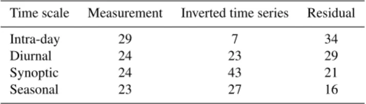
In order to identify the sources contributing to these terms, we perform a time scale analysis as described by Hogrefe et al. (2003) and Hogrefe et al. (2001). We use the Kolmogorov-Zurbenko filter to separate the time series ac-cording to the temporal scale of the signal. The concentra-tions are split into intra-day, diurnal, synoptic and seasonal components. Note that for simplicity, we use the same coef-ficients as Hogrefe et al. (2003), although that means that our categories include longer time scales because we have data on alternate hours rather than every hour. The contribution of each temporal component to the full time series is obtained by calculating the variance of each component as a fraction of the sum of the variances of all the components.
Table 6.Time scale analysis of the measurements, the inverted time series and the residual. This shows the percent of variance in the time series due to components with different time scales. The mea-surements contains variations at all time scales, but the inverted time series does not account sufficiently for hourly variations.
Time scale Measurement Inverted time series Residual
Intra-day 29 7 34
Diurnal 24 23 29
Synoptic 24 43 21
Seasonal 23 27 16
similar contributions from each category. In contrast, the in-verted time series is much lower on the intra-day component, which accounts for 7 % instead of 29 % of the variance. Cor-respondingly, the synoptic scale accounts for a greater frac-tion of the variance (43 % instead of 24 %). For the residual, the components are highest in the intra-day scale and lowest in the seasonal scale.
This demonstrates that the inverse model is missing some of the high frequency components of the time series. These are due to short spikes in concentrations, which are most likely to be local sources where the plume has not had as much time to dilute. This suggests that the method is more likely to underestimate sources that are close by. Conse-quently, it can be inferred that a significant fraction of the unaccounted mercury is due to local sources.
When the inverse method cannot match high frequency peaks, it compensates by increasing the background term to obtain similar average levels of GEM over the entire time period. This suggests that local sources which cannot be re-solved by the model contribute to the local and regional back-ground term. As a result, this analysis is in agreement with Rutter et al. (2008) who suggest that one third of GEM is from local point sources.
4.3 Lake, forest fire and volcano emissions
The results of this analysis suggest that the emissions of GEM from the lake surfaces are two times higher than those calculated in Sect. 2.4. As noted above, there is considerable spread in the measured concentrations of dissolved gaseous mercury. The inverse model suggests that average values may be towards the higher end of the reported range, well above the 30 pg l−1used in the calculations. This would suggest
av-erage fluxes in the range of 4 to 5 ng m−2h−1and total
emis-sions from the Great Lakes of 12 000 to 14 000 kg of GEM for the time period of the study.
Forest fires were found to have a clearly detectable sig-nal in the GEM time series, with total impacts around 30 % higher than the lake surface impacts. Most of these are due to emissions in the east domain which includes a large part of the midwest, the northeast and Southeastern Canada. The inverse model suggests that emissions from this area could
be underestimated by a factor of 3 to 4. The model further suggests that emissions in the north central domain could be underestimated by a factor of 2 to 3, but that estimates of the emissions form the south central and southeast domains are of the correct magnitude. The domains further away were found to have nil or variable impacts. This could be because there is not enough data in the inversion, either because those areas do not influence the measurement site often enough, or because the level of the impacts is too low relative to other sources. Finally, the FINN model estimated releases of 1383kg of mercury in WRF domain 2, close to the mea-surement site. The inverse model did not identify any im-pacts from these. This could be because local sources have short, sharp peaks which can easily suffer from mismatches between the model and the measurements or because the di-urnal distribution of the emissions is more important for lo-cal sources. As with the gridded emissions, the inverse model does a better job of identifying sources that are further away than near-field ones.
There was one large episode of elevated GEM concentra-tions starting on 12 November 2004 and lasting until the end of the month which is not accounted for in the inversion, see Fig. 10. Levels rose rapidly to between 4 and 6 ng m−3 and decayed slowly over the next 2 weeks. This suggests a large regional source, but the event is puzzling because it lasted over a variety of wind patterns with shifting air masses from both the north and the south. Volcanoes can emit large amounts of mercury during explosions (Bagnato et al., 2011) and could be a possible source. Mount St. Helens in Wash-ington State had renewed eruptions between September 2004 and December 2005 and could possibly be a factor in this event (Sherrod et al., 2008). We simulated forward emissions from the volcano using CAMx in combination with the large WRF domain used for forest fires. Although this source can-not be ruled out, the results did can-not provide strong evidence in support of this hypothesis.
Gr´ımsv¨otn in Iceland had a week long eruption starting on 1 November 2004 (Thordarson and Larsen, 2007). We per-formed forward particle simulations using FLEXPART based on wind fields from the Global Forecast System. Although the arrival time matched the episode in the time series, the simulated concentrations lasted much longer than the mea-sured episode itself. It would therefore seem that such a dis-tant source cannot be responsible for such a clearly defined event. Nevertheless, further analysis of this event may be warranted especially if it can be expanded with concurrent measurements from different sites.
5 Conclusions
of source strengths as well as source impacts at the measure-ment site. Using bootstrapping, the method further provided confidence intervals on the results.
Identifying local point sources is a particular challenge. The analysis therefore required a combination of analysis methods including meteorological analysis, concentration field analysis and time scale analysis to supplement the in-verse method.
Average GEM concentrations in Milwaukee were 2.5 ng m−3. 61 % of this is due to the global background concentration of 1.5 ng m−3. The inverse method ascribed 20 % to the local and regional background and did not account for another 6 %. Time scale analysis suggested that most of this is due to variations in concentrations on an hourly scale which could be attributed to local sources. The remaining 13 % was split as follows: 26 % from forest fires, 18 % from lake surface emissions and 56 % from local and regional sources covered by the inversion grid. Within this grid, the emissions estimate of the coal-fired power plants in the Ohio River Valley were in good agreement with current inventories. Sources in other areas were under-represented in the current inventories. In particular, local sources could be up to a factor of 4 or 5 higher, and sources in the southwest quadrant could be up to a factor of 2 higher. These sources may include waste disposal as well as metal processing. Overall, this study is consistent with Rutter et al. (2008) who suggest that there is a large urban excess of GEM in Milwaukee, and that one third of the GEM could be due to local sources.
The impacts of emissions from the lake surface and from forest fires could be clearly seen in the model inversion. These suggest that emissions from both of these sources are larger than predicted by current emissions models and that they contribute 2.5 % and 3.5 % to overall GEM levels in Milwaukee.
As the inversion uses a hybrid model, it is straightfor-ward to simulate candidate sources using a chemical trans-port model and include them in the analysis. Soil and vege-tation sources could be included in the same way as the lake surface sources. Further examples would depend on the lo-cation of the measurement site and could include testing the possibility of emissions from disparate sources such as melt-ing snow or the magnitude of emissions from gold minmelt-ing and underground coal fires.
Acknowledgements. This manuscript was made possible by EPA grant number RD-83455701. Its contents are solely the responsibil-ity of the grantee and do not necessarily represent the official views of the EPA. Further, the EPA does not endorse the purchase of any commercial products or services mentioned in the publication. The initial mercury measurements were funded by US EPA STAR Grant # R829798. We are also grateful to the US EPA for making the National Emissions Inventory and Toxic Release Inventory available, and to the US National Climatic Data Center for the
meteorological data. We are grateful to the two anonymous referees whose careful reviews improved the quality of this paper.
Edited by: R. Harley
References
Akagi, S. K., Yokelson, R. J., Wiedinmyer, C., Alvarado, M. J., Reid, J. S., Karl, T., Crounse, J. D., and Wennberg, P. O.: Emis-sion factors for open and domestic biomass burning for use in atmospheric models, Atmos. Chem. Phys., 11, 4039–4072, doi:10.5194/acp-11-4039-2011, 2011.
Ashbaugh, L. L., Malm, W. C., and Sadeh, W. Z.: A residence time probability analysis of sulfur concentrations at grand-canyon-national-park, Atmos. Environ., 19, 1263–1270, 1985.
Aster, R. C., Borchers, B., and Turber, C. H.: Parameter Estimation and Inverse Problems, Academic Press, second edn., 2012. Bagnato, E., Aiuppa, A., Parello, F., Allard, P., Shinohara, H.,
Li-uzzo, M., and Giudice, G.: New clues on the contribution of Earth’s volcanism to the global mercury cycle, Bull. Volcan., 73, 497–510, doi:10.1007/s00445-010-0419-y, 2011.
Bash, J., Miller, D., Meyer, T., and Bresnahan, P.: Northeast United States and Southeast Canada natural mercury emissions esti-mated with a surface emission model, Atmos. Environ., 38, 5683–5692, doi:10.1016/j.atmosenv.2004.05.058, 2004. Bash, J. O.: Description and initial simulation of a dynamic
bidi-rectional air-surface exchange model for mercury in Commu-nity Multiscale Air Quality (CMAQ) model, J. Geophys. Res.-Atmos., 115, doi:10.1029/2009JD012834, 2010.
Bash, J. O. and Miller, D. R.: A relaxed eddy accumulation system for measuring surface fluxes of total gaseous mercury, J. Atmos. Ocean. Technol., 25, 244–257, doi:10.1175/2007JTECHA908.1, 2008.
Brioude, J., Kim, W., Angevine, W. M., Frost, G. J., Lee, S.-H., McKeen, S. A., Trainer, M., Fehsenfeld, F. C., Holloway, J. S., Ryerson, T. B., Williams, E. J., Petron, G., and Fast, J. D.: Top-down estimate of anthropogenic emission inventories and their interannual variability in Houston using a mesoscale inverse modeling technique, J. Geophys. Res.-Atmos., 116, D20305, doi:10.1029/2011JD016215, 2011.
Bullock, Jr., O. R., Atkinson, D., Braverman, T., Civerolo, K., Das-toor, A., Davignon, D., Ku, J.-Y., Lohman, K., Myers, T. C., Park, R. J., Seigneur, C., Selin, N. E., Sistla, G., and Vija-yaraghavan, K.: The North American Mercury Model Inter-comparison Study (NAMMIS): Study description and model-to-model comparisons, J. Geophys. Res.-Atmos., 113, D17310, doi:10.1029/2008JD009803, 2008.
Carroll, M., Townshend, J., Hansen, M., DiMiceli, C., Sohlberg, R., and Wurster, K.: Vegetative Cover Conversion and Vegeta-tion Continuous Fields, in: Land Remote Sensing and Global En-vironmental Change: NASA’s Earth Observing System and the Science of Aster and MODIS, edited by: Ramachandran, B., Jus-tice, C. O., and Abrams, M., Springer-Verlag, doi:10.1007/978-1-4419-6749-7, 2011.