www.ann-geophys.net/25/1011/2007/ © European Geosciences Union 2007
Annales
Geophysicae
Spatial and temporal characteristics of poloidal waves in the
terrestrial plasmasphere: a CLUSTER case study
S. Sch¨afer1, K. H. Glassmeier1, P. T. I. Eriksson2, V. Pierrard3, K. H. Fornac¸on1, and L. G. Blomberg2
1Institut f¨ur Geophysik und extraterrestrische Physik, TU Braunschweig, Germany
2Space and Plasma Physics, School of Electrical Engineering, Royal Institute of Technology Stockholm, Sweden 3Belgian Institute for Space Aeronomy, Brussels, Belgium
Received: 20 December 2006 – Revised: 2 April 2007 – Accepted: 13 April 2007 – Published: 8 May 2007
Abstract. Oscillating magnetic field lines are frequently ob-served by spacecraft in the terrestrial and other planetary magnetospheres. The CLUSTER mission is a very suitable tool to further study these Alfv´en waves as the four CLUS-TER spacecraft provide for an opportunity to separate spa-tial and temporal structures in the terrestrial magnetosphere. Using a large scaled configuration formed by the four space-craft we are able to detect a poloidal Ultra-Low-Frequency (ULF) pulsation of the magnetic and electric field in order to analyze its temporal and spatial structures. For this purpose the measurements are transformed into a specific field line related coordinate system to investigate their specific ampli-tude pattern depending on the path of the CLUSTER space-craft across oscillating field lines. These measurements are then compared with modeled spacecraft observations across a localized poloidal wave resonator in the dayside plasma-sphere. A detailed investigation of theoretically expected poloidal eigenfrequencies allows us to specify the observed 16 mHz pulsation as a third harmonic oscillation. Based on this we perform a case study providing a clear identification of wave properties such as an spatial scale structure of about 0.67RE, the azimuthal wave numberm≈30, temporal evo-lution, and energy transport in the detected ULF pulsations.
Keywords. Magnetospheric physics (MHD waves and in-stabilities; Plasmasphere) – Space plasma physics (Waves and instabilities)
1 Introduction
Next to processes such as magnetic reconnection or colli-sionless shock waves the process of resonant mode coupling or magnetospheric field line resonance is a physical process
Correspondence to: S. Sch¨afer
(seb.schaefer@tu-bs.de)
whose knowledge we owe ground-based and in-situ obser-vation of space plasmas using spacecraft obserobser-vations. The theoretical basis for resonant coupling processes was estab-lished by Tamao (1965), Chen and Hasegawa (1974), and Southwood (1974) who were the first to provide a theoreti-cal framework to understand the resonant coupling between compressional waves with small azimuthal wave numberm and Alfv´en waves in an inhomogeneous plasma.
The physical resonant mode coupling can be understood considering electric current continuity. From Maxwell’s equations the following wave equation is derived for low-frequency waves:
∇ × ∇ ×E+µ0
∂j
∂t =0. (1)
HereE denotes the wave electric field, andj is the electric current density driving the wave. A magnetohydrodynamic wave in a homogeneous plasma carries polarization currents
jp =
1 µ0vA2
dE
dt , (2)
wherevA=B0/µ0ρ0defines the Alfv´en velocity andB0and
ρ0 denote the background magnetic field and the plasma
mass density, respectively. For an Alfv´en mode this polariza-tion current is curl-free in a plane whose normal is the back-ground magnetic fieldB0. The fast mode carries a
Observational evidence for the existence of such reso-nances was provided by e.g. Samson et al. (1971) and Walker et al. (1979) using ground-based and ionospheric observa-tions, respectively. Also spacecraft observations provide some evidence for the existence of field line resonances in the terrestrial magnetosphere (e.g. Engebretson and Cahill, 1981; Engebretson et al., 1986). The azimuthal variation of these observed resonances was found to be rather small; typ-ical azimuthal wave numbers are of the order ofm=5 (e.g. Olson and Rostoker, 1978). In the radial direction widths of standing Alfv´en waves are observed between 0.2RE and 1.6RE(e.g. Walker et al., 1979; Singer et al., 1982; Mitchell et al., 1990).
The source for the primary fast mode wave is in many oc-casions a Kelvin-Helmholtz instability of the magnetopause (e.g. Engebretson et al., 1997). A dominating wave damping mechanism for the coupled Alfv´en mode is Joule heating in the ionosphere (e.g. Glassmeier et al., 1984).
However, many ULF pulsation observations, though inter-preted as field line resonances, lag a definite proof of their resonant character as single spacecraft observations do not allow to demonstrate the spatial localization of the wave am-plitude and the typical 180◦ phase change of the toroidal component in radial direction. What is observed is usu-ally a spatial localization in the radial or poloidal compo-nent, not the toroidal component (e.g. Singer et al., 1979, 1982; Singer, 1982; Cramm et al., 2000). Furthermore, such poloidally localized waves exhibit large azimuthal wave numbers m≈50–150. For such largem-value ULF pulsations the field line resonance mechanism is a rather inefficient one (e.g. Kivelson and Southwood, 1986; Lee and Lysak, 1990) and cannot be used as an explanation to understand these poloidal resonances. Leonovich and Mazur (1990) give a simple reason for this: in the limitm→0 the azimuthal com-ponent of the wave vectorkφ is equal to infinity. But also the radial componentkr tends to infinity in case of an ideal resonance. Because of∇·B=0 the direction of the transverse magnetic field component is not defined.
The question thus arises on how to understand the spa-tial structure of poloidal ULF pulsations with largem val-ues. Observations from single spacecraft have only a limited value in providing the necessary experimental background to tackle this question. Due to spacecraft motion a separa-tion between spatial and temporal variasepara-tions is not possible. Temporal variations can be introduced by the dynamics of the wave source itself. They also reflect the described cou-pling processes which take a finite time to reach a steady state situation. Phase mixing as discussed in more detail by e.g. Mann and Wright (1995) thus causes significant tempo-ral variations and polarization changes which cannot be re-solved by single spacecraft measurements.
Here the four CLUSTER spacecraft (Escoubet et al., 1997) represent a very suitable tool to analyze magnetospheric ULF pulsations as shown in a recent study of poloidal ULF pul-sations by Eriksson et al. (2005b). These spacecraft move
through the magnetosphere on polar orbits forming various scaled configurations with distances between 0.016RE and 2.0RE. Compared to previous missions with one or two spacecraft the advantage of the CLUSTER mission consists in the availability of four measurement points either close to each other within the same region of interest or located in different regions. Due to its polar orbit the region close to the plasmapause is of particular interest. Here plasma condi-tions are more complex than in the outer region of the mag-netosphere as steep plasma density gradients, finite plasma beta, field line curvature, and the ring current may influ-ence the ULF pulsation wave field. Also, as the plasmapause is located deep in the magnetosphere wave sources are not necessarily associated with processes at the magnetopause. Rather local populations of energetic particles are generally accepted as a wave source of poloidal oscillations (Ozeke and Mann, 2001) leading to plasma instabilities such as the drift mirror (Hasegawa, 1969) and the bounce instabilitiy (South-wood et al., 1969; South(South-wood and Kivelson, 1982).
A suitable theoretical framework to interpret the spatial structure of poloidal oscillations with large m-values has been presented by e.g. Leonovich and Mazur (1990). Some of their results can be understood again considering the dif-ferent currents associated with the restoring forces influenc-ing the wave. For example, the influence of a finite plasmaβ can be incorporated in Eq. (1) by a diamagnetic current
jβ =∇
P×B0
B02 . (3)
Magnetic field line curvature introduces curvature currents
jc. If the background plasma carries a significant electric
currentJas observed in the ring current region a further cur-rent,
jJ =
(J×b)×B0
B02 , (4)
needs to be considered when solving Eq. (1); herebdenotes the magnetic field perturbation vector. This current describes forces associated with work done by the perturbed plasma against the current-carrying background.
Wave propagation outwards, however, is possible. As the local eigenfrequencies of toroidal and poloidal modes are dif-ferent any outward propagating large-mpoloidal wave may couple to a toroidal oscillation. Poloidal perturbations are related to toroidal transverse currents carrying the wave. As the azimuthal wave numbermis large this toroidal current changes sign rapidly also in azimuthal direction. Current continuity requires the transverse divergence of this current to be closed via field-aligned and poloidal currents. This causes coupling between the primary poloidal magnetic field perturbation and a secondary toroidal magnetic field oscilla-tion. If the local eigenfrequencies of the poloidal and toroidal oscillations match a local toroidal field line resonance occurs. Wave propagation is thus restricted to a region bounded by the poloidal turning point and the toroidal resonance point. This region thus defines a magnetospheric resonator or wave guide (Leonovich and Mazur, 1995).
This toroidal resonance is the true equivalent to the clas-sical field line resonance first described by Tamao (1965), Chen and Hasegawa (1974), and Southwood (1974). In case of the classical field line resonance the primary, low-mpoloidal wave is generated at the magnetopause, while the primary, large-mwave of the magnetospheric resonator field line resonance is generated within the resonator region.
The above discussion indicates that the radial structure of large-mpoloidal waves in the magnetospheric resonator will be more complex than that one of a classical field line resonance. A polarization change may happen between the poloidal inner turning point and the outer toroidal resonance. The spatial structure within the resonator needs to be consid-ered.
Furthermore, the outer boundary of the resonator can be another poloidal turning point, not a toroidal resonance, de-pending on plasma background properties (e.g. Vetoulis and Chen, 1994, 1996; Leonovich and Mazur, 1995; Denton and Vetoulis, 1998; Klimushkin, 1998a). The existence of two ra-dially arranged turning points suggests that a poloidal wave trapped in this kind of resonator can propagate in both di-rections, inward as well as outward. Detailed studies of the radial variations of the ULF wave field in magnetospheric resonator regions are thus desirable and will allow a deeper insight into the plasma physical processes there.
With the present study we intend to initiate a series of stud-ies on poloidal ULF waves in the outer region of the plasma-sphere/inner region of the magnetosphere. In this first report we shall demonstrate the complex spatio-temporal structure of wave fields as seen by the four CLUSTER spacecraft, in-troduce a new way of representing the observed wave field, and use the theoretical framework of Leonovich and Mazur (1990, 1993, 1995) and Klimushkin (1998a) to model the ob-served wave fields. Fluxgate magnetometer (FGM) measure-ments (Balogh et al., 2001) and electric field observations of the EFW instrument (Gustafsson et al., 2001) onboard CLUSTER are analyzed.
-1 0 1 2 3 4 5
XGSM [RE]
-4 -2 0 2 4
ZGSM
[R
E
]
September 15, 2002
PLASMASPHERE
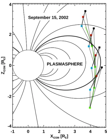
Fig. 1. The CLUSTER orbits in the dayside magnetosphere on 15 September 2002, 06:00, 07:00, 08:00 and 09:00 UT. The satel-lite move from south to north. The thick black line represents the plasmapause found atL=4.7.
2 Observations
A poloidal wave event has been detected onboard the CLUS-TER spacecraft on 15 September 2002 between 06:50 and 08:00 UT. The CLUSTER orbits during this time interval are displayed in Fig. 1. Field lines have been calculated using the Tsyganenko magnetospheric magnetic field model (Tsy-ganenko, 1995; Tsyganenko and Stern, 1996). The space-craft move from the southern dayside magnetosphere into the northern part of the magnetosphere with a velocity of vsc≈2 km/s. The spacecraft form a large scale tetrahedron with distances between 3000 km and 16 000 km. This config-uration provides for an opportunity to investigate ULF pulsa-tions simultaneously observed on different field lines by ap-plying a specific analysis method described in detail further down.
06:00 06:20 06:40 07:00 07:20 07:40 08:00 08:20 Time [UT]
0 1 2 3 4 5 6
U [V]
Spacecraft Potential C4
L=4.7 L=4.7
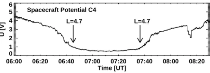
Fig. 2. Spacecraft potentialUdetected by Cluster C4. The arrows mark the times when spacecraft C4 crosses the assumed plasma-pause position atL=4.7 (06:45 and 07:37 UT).
entered the terrestrial plasmasphere and traversed the mag-netospheric resonator region discussed in the introduction.
To confirm this the position of the plasmapause is deter-mined using the dynamical simulations of plasmapause for-mation developed by Pierrard and Lemaire (2004) and Pier-rard and Cabrera (2005). This simulation uses the magneto-spheric electric field model E5D determined from dynamical proton and electron spectra measured on board the geosta-tionary satellites ATS5 and 6 (McIlwain, 1986). As the elec-tric field model depends only on theKpindex the simulation of the plasmapause formation is fully determined by this ac-tivity index.
For the given time interval we determine a radial dis-tance of the plasmapause in the magnetic equatorial plane of 4.7RE. The field line with the corresponding vertex is assumed as the plasmapause out of the equatorial plane and is indicated by the thick black line in Fig. 1. The assumed plasmapause location atL=4.7 is confirmed by the space-craft potential detected with the EFW instrument on board spacecraft C4 (Fig. 2). A decreased spacecraft potential indi-cates a higher electron density (Gustafsson et al., 2001; Ped-ersen et al., 2001). During the time interval analyzed here the solar wind conditions were quiet and stable which jus-tifies the assumption of a constant position of the plasma-pause. Except for one all satellites crossed the plasmapause in the Northern and Southern magnetic Hemisphere and thus moved into the dayside plasmasphere. Direct measurements of the electron density as well as ion density and plasma composition by the WHISPER (D´ecr´eau et al., 2001) and CIS (R`eme et al., 2001) instruments, respectively, onboard CLUSTER do not provide reliable observations for the time period of interest.
Observations used are 4s averaged magnetic and electric field measurements. The data are transformed into a Mean-Field-Aligned (MFA) coordinate system (er,eφ,ek), where
ekdenotes the unit vector in the direction of the background magnetic field,eφthe unit vector perpendicular to the plane spanned byekand the spacecraft position vector rsc. The unit vectorercompletes the right hand (er,eφ,ek) triad. The
coordinate system used is thus defined as follows:
er =eφ×ek (5)
eφ= h
Bi ×rsc
|hBi ×rsc|
(6)
ek= hBi
|B|. (7)
The mean magnetic fieldhBiis defined as a 512 s running av-erage magnetic field vector. In the MFA-system (br, bφ, bk) denote the magnetic disturbance field vectors. As we are only interested in field perturbations the mean value of the field-aligned component has been subtracted. The MFA-system allows to inspect also the polarization of the analyzed oscil-lations with (br, bφ, bk) approximately describing poloidal,
toroidal, and field-aligned components, respectively. To describe the electric field perturbations we furthermore assume thatE×B=0, i.e. no field-aligned electric field ex-ists. This allows to determine the third electric field nent from the two spacecraft spin-plane electric field compo-nents provided by the EFW instrument onboard CLUSTER. The vector (Er, Eφ,0) denotes the electric field in the MFA-system.
Observations from all four CLUSTER spacecraft for the time interval studied here are shown in Fig. 3, where the three upper panels display the magnetic field measurements and the two bottom panels the electric field measurements. To discriminate between the four spacecraft they are denoted as C1, C2, C3, and C4, respectively. The pulsation event is most clearly identified in records of spacecraft C3 and C4 with an onset time shift of about 30 min (Fig. 3). The other two spacecraft only detect minor field perturbations.
The frequency of the observed signal is in the range of a Pc4 pulsation,f≈16 mHz, observed in all components of the magnetic and electric field. The pulsation at spacecraft C3 is detected between 07:20 UT and 08:00 UT with transverse electric and magnetic field variations dominating. The ampli-tudes ofbφ andbr are modulated exhibiting a maximum of about 4 nT inbrand nearly constant field after 07:40 UT. The compressible component bk only shows a small amplitude fluctuation of the order of 1 nT. The electric field oscillates with a maximum amplitude of about 2 mV/m in both com-ponents and is almost zero between 07:37 UT and 07:48 UT. At spacecraft C4 the oscillation is seen 30 min earlier than at C3 and ceases at about 07:40 UT. Similar to the observa-tion in C3 the pulsaobserva-tion is observable in every component of
bandE. At C4 the radial amplitudebr is twice as large as the azimuthal amplitudebφand exhibits a peculiar two-wave packet modulation. The electric field oscillates again with an amplitude of 2 mV/m and is zero between 07:05 UT and 07:18 UT, whereas the amplitude increases in both compo-nents after 07:30 UT up to 5 mV/m inEφ and 10 mV/m in Er.
Further information about the observed signal is provided by the Poynting vectorS=µ1
0E×band the time-average en-ergy flux
hSi = 1
T
Z T
0
br
bφ 3 nT
b||
Er 6 mV/m
Eφ
06:50 07:00 07:10 07:20 07:30 07:40 07:50 Time [UT]
C1C2C3C4 August 7, 2003
Fig. 3. FGM and EFW measurements for the four Cluster
space-craft (C1: black, C2: red, C3, green, C4: blue), transformed into a Mean-Field-Aligned coordinate system. The bars denotes ampli-tudes of magnetic and electric field, respectively.
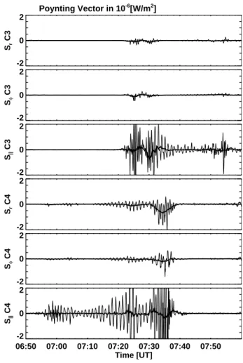
where T is the wave period (Fig. 4), in our caseT=63 s. A standing wave is indicated byhSi=0 and oscillating Poynting vectorS(Chi and Russell, 1998). This is especially observed until 07:20 UT in spacecraft C4. After that time the charac-ter of the energy flux changes with both transverse compo-nents now indicating a non-zero energy flux transverse to the ambient magnetic field. In particular, the large negative ra-dial componentSr corresponds to an inward directed energy transport indicating the presence of a propagating wave. The wave as observed by spacecraft C3 exhibits small transverse energy flux variationshSri andhSφi. The field parallel en-ergy flux is non-zero between 07:20 and 07:34 UT, but the oscillating component ofSkis dominant. A non-zero com-ponenthSkiis expected for a standing poloidal wave in case of asymmetric ionospheric conductances at the northern and southern footprint of the oscillating field lines (Ozeke et al., 2005). We conclude that at this time interval an almost stand-ing field line oscillation is observed by spacecraft C3 as well as spacecraft C4 between 06:50 and 07:20 UT.
-2 0 2
Sr
C3
-2 0 2
Sφ
C3
-2 0 2
S||
C3
-2 0 2
Sr
C4
-2 0 2
Sφ
C4
-2 0 2
S||
C4
Poynting Vector in 10-6[W/m2]
06:50 07:00 07:10 07:20 07:30 07:40 07:50 Time [UT]
Fig. 4. Components of the Poynting vectorSobserved by space-craft C3 and C4. The thick line represents the time-average energy flux.
3 Analysis and interpretation
3.1 Phenomenology of the wave activity
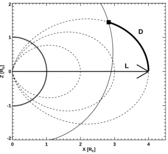
The main aim of the present study is to investigate spatial and temporal structures of poloidal Alfv´en waves. In princi-ple, this requires a 4-D-representation of the measurements made. To approach this requirement we introduce a special coordinate system, the L-D-M coordinate system, schemati-cally shown in Fig. 5. The coordinate L resembles the McIl-wain Parameter (McIlMcIl-wain, 1966) and describes the distance of the vertex of a specific field line with respect to the center of the Earth in units ofRE. To identify the field line for a given point in space the Tsyganenko 96 model (Tsyganenko, 1995; Tsyganenko and Stern, 1996) is used.
0 1 2 3 4
X [RE]
-2 -1 0 1 2
Z [R
E
] L
D
Fig. 5. Schematic illustrating the L-D-M coordinate system. The
spacecraft positions are marked by rectangles, the dotted lines rep-resent magnetic field lines.
coordinate, M, describes the magnetic local time (MLT) at which the measurements are taken.
The orbital coordinates of the different spacecraft are transformed into this L-D-M coordinate system, fluctuations of the electromagnetic field are still represented using the Mean-Field-Aligned coordinate system. At first we concen-trate on the actual observations ofbr andhSri in the L-D plane as seen in the upper panels of Fig. 6. Effects of minor changes in the M coordinate (lowest panel of Fig. 6) are dis-cussed later. For the representation ofbran analytic signal or Carson-Gabor representation (e.g. Glassmeier, 1980; Glass-meier and Motschmann, 1995) is used, which allows to de-termine instantaneous amplitude and phase of the given time series. As the ULF signals to be analyzed here are rather reg-ular the analytic signal representation is a very suitable tool. The thickness of the lines denoting the spacecraft positions in the first panel of Fig. 6 represents the instantaneous ampli-tude or signal envelope of the dominant radial component of the magnetic field oscillation. The thickness of the lines in the second panel of Fig. 6 is related to the radial component of the time averaged energy fluxhSri. The vertical black line in Fig. 6 represents the plasmapause position, previously also given in Fig. 1. Wave activity occurs preferentially within the plasmasphere.
In the present case study each spacecraft covers different ranges of L-values. The magnetic equator (D=0) is crossed by spacecraft C4 at the field line with its vertex atL=4.1, C3 atL=4.35, C2 at L=4.45, and C1 at 4.77, that is the four spacecraft cover a radial extent of about 0.67RE, a value comparable to earlier estimates of the radial extent of magne-tospheric pulsations. Therefore, the configuration is suitable to analyze the poloidal oscillation covered spatial region.
Information about the time at which a spacecraft crossed a specific field line is of particular interest. Spacecraft posi-tions at five selected times, labeled by roman numbers, are marked by squares in Fig. 6. These times have been selected as they correspond to those times spacecraft C4 and C3 cross the L=4.22 and L=4.4 field lines in the Southern and North-ern Hemisphere and the time spacecraft C4 detects the max-imum, radially directed energy flux.
At time I spacecraft C4 observed an amplitude maxi-mum atL=4.22; the wave amplitude decreased while space-craft C4 moved to lower L-values and increased after it crossed the magnetic equatorD=0RE. Spacecraft C1 and C2 were located far away from this field line atL>4.45 and did not detect pulsations as seen in the magnetic and electric field measurements (Fig. 3). We conclude that at time I the radial spatial extent of the pulsation event was too small to be observed by C1 and C2. Afterwards both spacecraft move further apart from the region of interest and in the following we concentrate on the observations of spacecraft C3 and C4. C3 was still too far away from the region of interest to detect any ULF signal at time I.
At time II another amplitude maximum was observed by C4 at the same field lineL=4.22 as at time I. This clearly indicates the existence of a radially localized wave structure along this field line oscillating for at least 24 min. At time II a pulsation was also detected by spacecraft C3, but atL=4.5 indicating a more complex radial structure of the wave field observed by the two satellites.
At time III C3 and C4 were located at the same field line shellL=4.4, but at slightly different M values. Approaching this field line shell C3 saw an increasing amplitude, indicat-ing a localized wave packet. At the same time C4, movindicat-ing towards the plasmapause only detected a minor change of the field amplitude. This difference in the amplitude behav-ior might be due to rapid azimuthal variations of the wave field.
Assuming an azimuthal variationb, E∝exp(imφ)the az-imuthal wave numbermcan be determined from the mea-sured phase difference, 1ψ, between radial magnetic field variations seen at C3 and C4 (e.g. Eriksson et al., 2005a):
m=1ψ
1φ. (9)
Here 1φ is the azimuthal distance between C3 and C4; at time III 1φ=3.18◦. Comparing time series of both spacecraft around time III the phase difference1ψ is esti-mated. The time difference1t between minima and max-ima, respectively, is about 20 s (Fig. 7), which corresponds to 1ψ≈100◦; thusm≈30. Such large azimuthal wave numbers are expected for poloidal oscillations (e.g. Radoski, 1967) and observed by Eriksson et al. (2005b) recently.
-2 -1 0 1 2
POSITION ALONG FIELD LINE D [R
E
]
MAGNETIC FIELD
PLASMASPHERE
PLASMAPAUSE
I
I
I
II II
III III
IV
IV
V
-2 -1 0 1 2
POSITION ALONG FIELD LINE D [R
E
]
POYNTING FLUX
PLASMASPHERE
PLASMAPAUSE
I
I
I
II II
III III
IV
IV
V
C1
C2
C3
C4
September 15, 2002
4.0 4.2 4.4 4.6 4.8 5.0
L SHELL 11.0
11.5 12.0
M
Fig. 6. Positions of the CLUSTER spacecraft in the L-D coordinate system at different times, where the squares mark the positions of each
spacecraft. Time I corresponds to 06:58:38 UT, time II to 07:23:42 UT, time III to 07:30:22 UT, time IV to 07:34:22 UT and time V to 07:50:06 UT. The arrows show the flight direction of the CLUSTER satellites. The thickness of the lines are related to the amplitude of the radial oscillation of the magnetic fieldbr (upper panel) and the radial component of the time averaged Poynting vectorhSri(second panel).
The bottom panel shows the orbit in the L-M plane, where M corresponds to the magnetic local time MLT.
located at other field lines. This period of regular oscillations ceased when C4 reached the plasmapause region.
Between time I and time III the time averaged Poynting vectorhSiis close to zero indicating the existence of a stand-ing wave field structure. Afterwards spacecraft C4 observes an increasing radial energy flux with its maximum at time IV located at L=4.55 and D=1.4RE. At the same time
-4 -2 0 2 4
Br
C3 [nT]
07:29:00 07:29:30 07:30:00 07:30:30 07:31:00 07:31:30
-4 -2 0 2 4
Br
C4 [nT]
t
∆ ∆t
Fig. 7. Time series ofbr for spacecraft C3 (top) and C4 (bottom)
between 07:29 and 07:32 UT, where both satellites cross the same L-shell at different azimuthal positions M.
towards lower L shells; this is a probable explanation for the observed radially inward directed energy flux.
At time V spacecraft C3 again crossed the L=4.4 field line. However, the amplitude was smaller than during the southern crossing, which indicates a temporal variation of the pulsa-tion activity rather than a spatial one. All other spacecraft had already left the activity region at this time.
3.2 Wave frequency
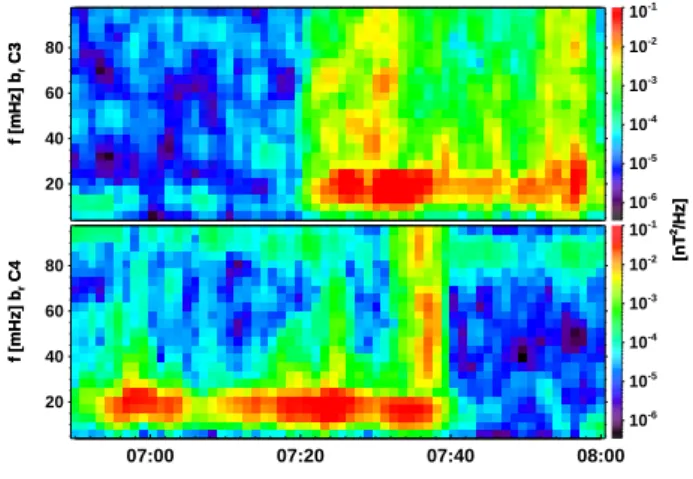
Phenomenological characteristics of the waves observed in the outer region of the plasmasphere are quite complex as discussed above. The wave frequency, however, is rather stable at fobs=16 mHz during the time spacecraft C3 and
C4 traversed this region, as seen in the dynamic spectra of the radial magnetic field component br (Fig. 8). Due to the radial spacecraft motion a frequency constant in time is equivalent to a uniform frequency with respect to mag-netic L shells, which has been previously observed and dis-cussed for poloidal wave events in outer magnetospheric re-gions (L>6) by Denton et al. (2003). Contrary to that the fre-quency of toroidal waves is expected to have aLdependence and consequently the radial structure of the here observed poloidal wave event cannot be explained by the field line res-onance mechanism. Details of the radial structure of poloidal waves can be gained by comparing the observed frequency with the radial profile of theoretically expected poloidal and toroidal eigenfrequencies (e.g. Denton and Vetoulis, 1998; Klimushkin, 1998b).
Theoretically expected toroidal eigenfrequenciesωT and eigenperiods TA of magnetospheric field lines can be
es-timated using the time of flight method (Warner and Orr, 1979):
ωT = 2π N
TA ;
TA=2
Z N
S ds vA
. (10)
Here N is the harmonic number of the field line standing os-cillation, ds is an increment of length along the field line
20 40 60 80
10-6
10-5
10-4
10-3
10-2
10-1
f [mHz] b
r
C3
f [mHz] b
r
C4
[nT
2/Hz]
20 40 60 80
10-6
10-5
10-4
10-3
10-2
10-1
f [mHz] b
r
C3
f [mHz] b
r
C4
[nT
2/Hz]
07:00 07:20 07:40 08:00
Fig. 8. Dynamic spectra of the radial magnetic field components brof the spacecraft C3 (top) and C4 (bottom) observations.
and the integration limits are the northern and southern iono-sphere. The Alfv´en velocity vA(s) along the field line is given byvA(s)=B(s)/√µ0ρ(s).
Poloidal eigenfrequencies ωP can be determined in the WKB approximation following Klimushkin (1998a) and Klimushkin (1998b):
ωP =ωT −ωgeom+ωβ. (11)
Hereωgeomdescribes the influence by the field line curvature
of a field line and is given by ωgeom=
1 2π N
Z N
S vA
∂2
∂s2(lnh)ds, (12)
wherehis a geometric factor depending on the coordinate system used (for details see Klimushkin, 1998a). The term ωβtakes into account the influence of finite but small values of the plasmaβ and resulting equilibrium currents J per-pendicular to the magnetic field in the equatorial plane, e.g. magnetospheric ring currents:
ωβ = 1 2π N
Z N
S 2vA
R µ0J
B +
2vMS2 Rv2A
!
ds. (13)
HereR is the field line curvature radius. The slow magne-tosonic velocityvMS is given by vMS=vSvA(vS2+v2A)−1/2, wherevS denotes the sound velocity. For simplicity dipole field lines are assumed to calculate the radius of curvatureR and the geometric factorh, an assumption well justified for plasmaspheric field lines. The coordinate system of Eq. (13) follows the definiton in Klimushkin (1998a). Here positive values ofJcorrespond to currents directed eastward.
0.0 0.2 0.4 0.6 0.8
plasma β
3 4 5 6 7
L shell 0
5 10 15 20 25
plasma pressure P [nPa]
-5 -4 -3 -2 -1 0 1
current
density J [10-9
Am-2
]
3 4 5 6 7
L shell 1
2 3 4
5 plasma density ρ [10-18
kgm-3
]
Fig. 9. Profiles of plasma properties. Plasma pressure and plasma βare assumed for quiet geomagnetic activity (Lui and Hamilton, 1992). The current density is obtained from the Tsyganenko ’96 model. Positive values ofJ⊥correspond to a current directed east-ward. The plasma density is calculated from modeling the electron number density (Carpenter and Anderson, 1992).
The latter can be determined using the Tsyganenko model of (Tsyganenko and Stern, 1996; Tsyganenko and Peredo, 1994) for given parameters such asDst=−19 nT and the dy-namic pressure of the solar windpdyn=0.85 nPa. We assume
typical distributions for plasmaβand isotropic plasma pres-sure (P⊥=Pk) as described e.g. by Lui and Hamilton (1992). To proof consistency with the Tsyganenko model the radial profile of the current densityJ is also derived from the given plasma pressure distribution by (Lui et al., 1987)
J⊥= −1 B
∂P
∂L. (14)
Here positiveJ⊥denotes westward current. We found good agreement between the current derived from Eq. (14) and the ring current of the Tsyganenko model. Profiles ofβ,P and J⊥are shown in Fig. 9.
The Tsyganenko 96 model (Tsyganenko and Stern, 1996) is used to calculate the magnitude of the magnetic fieldB(s) for a given field line. The plasma number density along the field line is assumed as a power law (Cummings et al., 1969) with an exponent α=1 typical for the plasmasphere (e.g. Goldstein et al., 2001; Denton et al., 2004):
n(s)=neq
LR
E r
α
. (15)
Herer is the geocentric distance to a point on the field line and the number density in the equatorial plane neq can be obtained from the model of Carpenter and Anderson (1992). Influences onneqdue to complex features of the plasmapause formation such as plasma plumes or shoulders (e.g. Pierrard and Lemaire, 2004; Goldstein, 2006) are not predicted by the
2.5 3.0 3.5 4.0 4.5 5.0 5.5
L shell 0
10 20 30 40
Eigenfrequencies f
T
, fP
[mHz]
1 2 3 4 harmonic number N
mcorr = 3
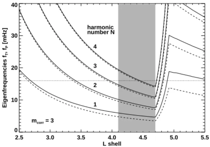
Fig. 10. Profiles of the poloidal eigenfrequenciesfP (solid line )
and toroidal eigenfrequenciesfT (dashed line) of magnetospheric
field lines calculated for harmonic numbers N=1, ...,4 and the mass correction factormcorr=3. The dotted line marks the observed frequencyf=16 mHz.The grey shaded background marks L-shells crossed by spacecraft C3 and C4 during the analyzed time interval.
applied simulation of the plasmapause formation, addition-ally approved by the observed spacecraft potential (Fig. 2). The plasma of the plasmasphere is composed of hydrogen and heavier ions such as helium and oxygen. This requires a mass correction factormcorr to calculate the plasma mass
densityρ(s)=n(s)mcorrmpaccurately, wherempis the
pro-ton mass. A typical plasmaspheric plasma is composed of 55% H+, 40% He+and 5% O+(Berube et al., 2005) leading to a mass correction ofmcorr≈3.
With these assumptions and model values the eigenfre-quencies of the fundamental poloidal and toroidal field line oscillation,fP=ωP/2π andfT=ωT/2π, as well as the fre-quencies of its harmonicsN=2, ...,4 have been calculated for L shells in the range [2.5,5.5]RE (Fig. 10). At L shells L=[4.1,4.7], where spacecraft C3 and C4 observe the described pulsation activity, poloidal eigenfrequencies are larger than the toroidal eigenfrequencies; the non zero plasmaβleads toωβ>0. The geometric contribution,ωgeom,
is always larger than zero forα=6. However, if we assume α6=6, negative values for ωgeom are well possible. In the
present caseα=1 is the best guess and we findωgeom<0 for
certain radial distances. This leads toωP>ωT in these re-gions.
The theoretical framework predicts the existence of a re-gion transparent for poloidal waves near a minimum offP only if the conditionfP<fobs<fT is satisfied (Klimushkin et al., 2004). In contrast to that we foundfT<fP<fobsin the
pulsation is localized within such a wave transparency region despite the contradiction between observation and theory. A possible reason for this discrepancy is the negative value of ωgeomdue to the assumed exponentα=1 in Eq. (15), as
dis-cussed above. As the conditionωgeom>ωβ is necessary to obtain a poloidal eigenfrequency smaller than the toroidal (see Eq. 11), we speculate that Eq. (12) is inappropriate in case of α=1. Apparently further efforts are necessary to improve the applied WKB approximation of the theoretical framework using the constraintα=1.
However, we suggest that Fig. 10 reflects the radial width of the poloidal resonator (e.g. Leonovich and Mazur, 1993). The outer boundary coincides with the plasmapause atL≈4.7 and the inner boundary depends on the harmonic numberN. Since spacecraft C4 observes the pulsation even atL=4.1, we exclude the fourth harmonic oscillation, which has the inner resonance surface located atL≈4.2. The ob-servations described in the L-D coordinate system (Fig. 6) reveal a symmetric amplitude structure relative to the mag-netic equatorD=0REsuggesting an oscillation with an odd harmonic number. For the fundamental oscillationN=1 the spatial extent of the oscillating structure would be more than 2RE. Consequently, we suggest that the observed pulsation is a third harmonic oscillation with a spatial extent of approx-imately 0.7RE.
3.3 Modeling the spatio-temporal structure
For further understanding of the observed pulsation event and to reach a deeper insight into its spatio-temporal structure we present a simple model for the spatio-temporal characteris-tics of the wave which is fitted to the actually observed data for better comparison. The dominant poloidal magnetic field component is given by
br,model=b0·A(D, φ)·B(L)·C(t ). (16)
HereA(D, φ) describes the spatial structure along the field line and in the azimuthal direction,B(L)the spatial structure in the radial direction across L-shells, andC(t )the temporal evolution of the wave amplitude. All three amplitude func-tions are normalized to 1, so that the maximum amplitude of the modeled signal is given byb0.
The model assumes a standing wave along the background magnetic field line:
A(D, φ)=sin(kkD+mφ)·cos(ωPt ). (17) This functional form describes odd mode oscillations with kk denoting the field parallel wave number. Wave fre-quency ωP=2πfP and azimuthal wave number m are de-termined using the observations. As mentioned in Sect. 2 the change in the azimuthal spacecraft position1φ=1Mis small, but since we foundm≈30, the phase variation1(mφ) is not negligible. The parallel wavelength λk=2π/ kk de-pends on the length of the field line l and the harmonic numberN: λk=2l/N. The lengths of the field lines with
vertices between L=4.1RE and L=4.7RE are between l=9.4 andl=10.0RE. Assuming a third harmonic oscilla-tion as discussed above gives one wavelengths in the range λk=[6.3,6.7]REor wave numberskk=[0.94,1.00]RE−1.
The transverse variation of the wave field is described by multiplying the standing wave (Eq. 17) with an amplitude functionB(L). Leonovich and Mazur (1990) have shown that for a poloidal wave resonator the functionB(L)can be approximated by the product of a Hermitian polynomialHn of order n and a Gaussian:
B(L)=Hn(ξ )exp(−ξ2/2), (18)
whereξ=(L−LR)/σ. HereLRdenotes the location of max-imum wave amplitude andσdescribes the radial width of the wave field within the wave guide region, respectively. For a zeroth order Hermitian polynomial (n=0) the radial struc-tureB(L)is just given by a Gaussian as already observed for poloidal pulsations (e.g. Cramm et al., 2000).
Using higher order Hermitian polynomials allows to de-scribe a more complex wave field variation in radial direction as the number of extrema of the polynomial used is equal to n+1. Figure 6 exhibits two amplitude maxima atL=4.22 and L=4.40RE. The first one at L=4.22RE is detected twice by spacecraft C4 when it crosses the corresponding field line below and above the magnetic equator. The sec-ond one atL=4.40RE is detected only by C3. Due to this observation a first order Hermitian polynomial withn=1 is used in Eq. (18).
The amplitude maxima on the field line L=4.22RE are observed atD=−0.7REandD=0.9RE, that is almost sym-metric with respect to the magnetic equator. Assuming a standing wave, one would expect nearly the same pulsation strength for both crossings. However, the opposite is ob-served with the northern maximum displaying a somewhat small amplitude value (Fig. 6). This is either due to the sym-metry point not coinciding with the magnetic equator or the result of a temporal evolution of the wave field, approximated by a Gaussian functionC(t )with its maximum at 07:32 UT corresponding to the observed maximum of the signal. An increasing amplitude can be explained by e.g. drift bounce resonance effects, as described in Klimushkin and Mager (2004). On the other hand, wave dissipation at the iono-spheric boundaries leads to a decreasing pulsation amplitude. The aim of our modeling effort is to characterize the am-plitudeb0, the activity maximum positionLRand its width
σ. Varying these model parameters the best correspon-dence between modeled signal and the actual observations of spacecraft C3 and C4 have been reached forLR=4.35RE, σ=0.1RE, m=30, and b0=6.5 nT. A comparison of both
07:00 07:20 07:40 08:00 Time [s]
0 1 2
3 CLUSTER C3
07:00 07:20 07:40 08:00
Time [s] CLUSTER C4
Fig. 11. Comparison between measurement of thebr (solid line)
component and the model of the wave fieldbr,model(dashed line).
seen in C3 after 07:35 UT. Observations between 07:10 and 07:35 UT are well represented by the modeled signal. Es-pecially the modeled shape of the second amplitude peak in spacecraft C4 is in a good agreement with the observed am-plitude modulation.
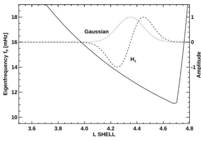
Figure 12 shows a comparison between the modeled ra-dial variation of the wave field and the rara-dial variation of the poloidal eigenfrequency. It is remarkable to see that the wave activity region as modeled well coincides with the wave guide region identified as the trough in the poloidal eigenfre-quency variation. From the modeled signal we also infer that the total width of the wave guide is about 0.6RE, which cor-responds to the observed extend of the wave activity region.
It should be noted that the time interval between 07:30 and 07:40 UT of the spacecraft C4 observation is excluded from our modeling efforts as at this time a propagating wave is detected (Figs. 4 and 6) and the assumption of a standing wave is not suitable in this region.
Differences between model and measurements originate from several sources. First, the Hermitian function used to describe the radial structure is based on the assumption of a wave guide symmetric to the point of minimum eigenfre-quency. This assumption is not fully consistent with the ac-tual variation of the poloidal eigenfrequency. Second, theo-retical studies such as presented by Klimushkin and Mager (2004) assume a time harmonic time variation without any amplitude modulation. A more realistic temporal evolution of the wave field is not incorporated in current theoretical treatments. We think that this oversimplification is the main reason for discrepancies between model and observation. However, similarities found suggest that the theoretical as-sumptions allow for explaining the observed amplitude mod-ulation, at least after the wave field is fully developed and before it collapsed due to ionospheric dissipation.
4 Conclusions
A new representation of magnetic field measurements has been developed which allows a very convenient graphical display of CLUSTER multi-spacecraft observations helping
3.6 3.8 4.0 4.2 4.4 4.6 4.8
L SHELL 10
12 14 16 18
Eigenfrequency f
P
[mHz]
H1
Gaussian
-1 0 1
Amplitude
Fig. 12. Comparison between the modeled radial variation and the
radial variation of the poloidal eigenfrequency.
to visualize spatial and temporal effects due to spacecraft mo-tion. This new visualization tool has been applied to ULF pulsation observations in the terrestrial dayside plasmasphere and a region of a poloidal standing wave was detected and analyzed.
The field line oscillations analyzed were observed in the time interval 15 September 2002, 06:50–08:00 UT. The large scaled spacecraft configuration during this interval has en-tailed the possibility to record the pulsation event over a time period of around 70 min in spacecraft C3 and C4. During this time the spacecraft crossed the oscillating field lines twice during their inbound and outbound approaches to the Earth on an almost polar orbit.
Analyzing the phase differences between signals observed by two spacecraft while passing the same L shell has given us the possibility to estimate the azimuthal wave number; we foundm≈30. Accordingly, a poloidal polarized oscillation withm≫1 was detected.
To describe temporal and spatial properties of the observed wave field we have used a theoretical framework developed by Leonovich and Mazur (1990, 1993, 1995) and Klimushkin (1998a). A profile of poloidal eigenfrequenciesfP was eval-uated based on realistic assumption concerning plasma com-position and plasma properties in the region of interest. Com-paring with the observed frequencyfobs=16 mHz has
sug-gested a third harmonic oscillation.
The wave field was found localized near the minimum of fP bounded by turning pointsfP=fobsat the plasmapause
and within the plasmasphere, respectively. In this region the existence of a localized pulsation is not fully predicted by theory. Hence, further efforts on the theoretical description of plasmaspheric ULF pulsations are necessary.
together with a complex radial structure extended to higher L-shells. The wave event is localized in radial direction. However, this localization is not due to any resonant mode coupling, but thought to be the result of the wave field en-countering two poloidal turning points, much as predicted by Klimushkin (1998a). The spatial extent of the wave field area is around 0.6RE, which confirms previous observations of plasmaspheric ULF pulsations (Ziesolleck et al., 1993; Menk et al., 1999). The radial structure was described by a spe-cific function as suggested by Leonovich and Mazur (1990). In addition to the standing structure the investigation of the wave Poynting vector has clearly exposed the existence of an inward directed, propagating wave.
Comparing observations with the modeled standing os-cillation exposes strengths and weak points of the applied model and its theoretical basis. For the given situation of a solely poloidal polarized field line oscillation a theory is cur-rently unavailable specifying the temporal evolution of such a wave field. Thus, the measured pulsation can only be re-produced in parts by the modeled standing structure.
Our future efforts will concentrate on the performance of further event studies of ULF pulsations localized within plasmasphere and plasmapause. We intend to analyze these events with the method introduced by the present work. In addition to that we aim for the development of a statistical survey of properties of Alfv´enic waves in the terrestrial mag-netosphere. For these purposes the CLUSTER mission is an appropriate tool providing us with an extensive amount of magnetic and electric field data over a time range of more than five years.
Acknowledgements. This work was financially support by the
Ger-man Ministerium f¨ur Wirtschaft und Technologie and the Deutsches Zentrum f¨ur Luft- und Raumfahrt under contract 50OC0103. Part of this work was financially supported by INTAS under contract 05-1000008-7978.
Topical Editor I. A. Daglis thanks S. Buchert and another referee for their help in evaluating this paper.
References
Balogh, A., Carr, C. M., Acuna, M. H., and Dunlop, M. W.: The Cluster magnetic field investigation: overwiew of in-flight perfo-mance and initial results, Ann. Geophys., 19, 1207–1217, 2001, http://www.ann-geophys.net/19/1207/2001/.
Berube, D., Moldwin, M. B., Fung, S. F., and Green, J. L.: A plas-maspheric mass density model and constraints on its heavy ion concentration, J. Geophys. Res. (Space Physics), 110, A04 212, 1–5, doi:10.1029/2004JA010684, 2005.
Carpenter, D. L. and Anderson, R. R.: An ISEE/Whistler model of equatorial electron density in the magnetosphere, J. Geophys. Res., 97, 1097–1108, 1992.
Chen, L. and Hasegawa, A.: A theory of long-periodic magnetic pulsations, 1. Steady excitation of field line resonances, J. Geo-phys. Res., 79, 1024–1032, 1974.
Chi, P. J. and Russell, C. T.: Phase skipping and Poynting flux of continuous pulsations, J. Geophys. Res., 103, 29 479–29 492, 1998.
Cramm, R., Glassmeier, K. H., Othmer, C., Fornacon, K. H., Auster, H. U., Baumjohann, W., and Georgescu, E.: A case study of a ra-dially polarized Pc4 event observed by the Equator-S satellite, Ann. Geophys., 18, 411–415, 2000,
http://www.ann-geophys.net/18/411/2000/.
Cummings, W. D., O’Sullivan, R. J., and Coleman, P. J.: Standing Alfv´en Waves in the Magnetosphere, J. Geophys. Res., 74, 778– 793, 1969.
D´ecr´eau, P. M. E., Fergeau, P., Krasnoselskikh, V., Le Guirriec, E., L´evˆeque, M., Martin, P., Randriamboarison, O., Rauch, J. L., Sen´e, F. X., S´eran, H. C., Trotignon, J. G., Canu, P., Cornil-leau, N., de F´eraudy, H., Alleyne, H., Yearby, K., M¨ogensen, P. B., Gustafsson, G., Andr´e, M., Gurnett, D. C., Darrouzet, F., Lemaire, J., Harvey, C. C., Travnicek, P., and Whisper Exper-imenters group: Early results from the Whisper instrument on Cluster: an overview, Ann. Geophys., 19, 1241–1258, 2001, http://www.ann-geophys.net/19/1241/2001/.
Denton, R. E. and Vetoulis, G.: Global poloidal mode, J. Geophys. Res., 103, 6729–6740, doi:10.1029/97JA03594, 1998.
Denton, R. E., Lessard, M. R., and Kistler, L. M.: Radial localiza-tion of magnetospheric guided poloidal Pc 4-5 waves, J. Geo-phys. Res. (Space Physics), 108, SMP 4, 1–10, doi:10.1029/ 2002JA009679, 2003.
Denton, R. E., Menietti, J. D., Goldstein, J., Young, S. L., and An-derson, R. R.: Electron density in the magnetosphere, J. Geo-phys. Res. (Space Physics), 109, A09 215, 1–14, doi:10.1029/ 2003JA010245, 2004.
Engebretson, M., Glassmeier, K.-H., Stellmacher, M., Hughes, W. J., and L¨uhr, H.: The dependence of high-latitude Pc5 wave power on solar wind velocity and on the phase of high-speed solar wind streams, J. Geophys. Res., 103, 26 271–26 284, doi:10.1029/97JA03143, 1997.
Engebretson, M. J. and Cahill, L. J.: Pc5 pulsations observed during the June 1972 geomagnetic storm, J. Geophys. Res., 86, 5619–
5631, doi:10.1029/0JGREA0000860000A7005619000001,
1981.
Engebretson, M. J., Zanetti, L. J., Potemra, T. A., and Acuna, M. H.: Harmonically structured ULF pulsations observed by the AMPTE CCE magnetic field experiment, Geophys. Res. Lett., 13, 905–908, 1986.
Eriksson, P. T. I., Blomberg, L. G., and Glassmeier, K.-H.: Cluster satellite observations of mHz pulsations in the dayside magneto-sphere, Adv. Space Res., 23, 2679–2685, doi:10.1016/j.asr.2005. 04.103, 2005a.
Eriksson, P. T. I., Blomberg, L. G., Walker, A. D. M., and Glass-meier, K.-H.: Poloidal ULF oscillations in the dayside magneto-sphere: a Cluster study, Ann. Geophys., 23, 2679–2685, 2005b. Escoubet, C. P., Schmidt, R., and Goldstein, M. L.: Cluster -
Sci-ence and Mission Overview, Space Sci. Rev., 79, 11–32, 1997. Glassmeier, K. H.: Magnetometer array observations of a giant
pul-sation event, Journal of Geophysics Zeitschrift Geophysik, 48, 127–138, 1980.
Glassmeier, K. H., Volpers, H., and Baumjohann, W.: Ionospheric Joule dissipation as a damping mechanism for high latitude ULF pulsations: Observational evidence, Planet. Space Sci., 32, 1463–1466, 1984.
Goldstein, J.: Plasmasphere Response: Tutorial and Review of Re-cent Imaging Results, Space Science Reviews, 124, 203–216, doi:10.1007/s11214-006-9105-y, 2006.
Goldstein, J., Denton, R. E., Hudson, M. K., Miftakhova, E. G., Young, S. L., Menietti, J. D., and Gallagher, D. L.: Latitudinal density dependence of magnetic field lines inferred from Polar plasma wave data, J. Geophys. Res., 106, 6195–6202, doi:10. 1029/2000JA000068, 2001.
Gustafsson, G., Andr´e, M., Carozzi, T., Eriksson, A. I., F¨althammar, C.-G., Grard, R., Holmgren, G., Holtet, J. A., Ivchenko, N., Karlsson, T., Khotyaintsev, Y., Klimov, S., Laakso, H., Lindqvist, P.-A., Lybekk, B., Marklund, G., Mozer, F., Mur-sula, K., Pedersen, A., Popielawska, B., Savin, S., Stasiewicz, K., Tanskanen, P., Vaivads, A., and Wahlund, J.-E.: First results of electric field and density observations by Cluster EFW based on initial months of operation, Ann. Geophys., 19, 1219–1240, 2001,
http://www.ann-geophys.net/19/1219/2001/.
Hasegawa, A.: Drift Mirror Instability in the Magnetosphere, Phys. Fluids, 12, 2642–2650, 1969.
Kivelson, M. G. and Southwood, D. J.: Coupling of global magne-tospheric MHD eigenmodes to field line resonances, J. Geophys. Res., 91, 4345–4351, 1986.
Klimushkin, D. and Mager, P.: The spatio-temporal structure of impulse-generated azimuthalsmall-scale Alfv´en waves interact-ing with high-energy charged particles in the magnetosphere, Ann. Geophys., 22, 1053–1060, 2004,
http://www.ann-geophys.net/22/1053/2004/.
Klimushkin, D., Mager, P., and Glassmeier, K.: Toroidal and poloidal Alfv´en waves with arbitrary azimuthal wavenumbers in a finite pressure plasma in the Earth’s magnetosphere, Ann. Geo-phys., 22, 267–287, 2004,
http://www.ann-geophys.net/22/267/2004/.
Klimushkin, D. Y.: Resonators for hydromagnetic waves in the magnetosphere, J. Geophys. Res., 103, 2369–2376, doi:10.1029/ 97JA02193, 1998a.
Klimushkin, D. Y.: Theory of azimuthally small-scale hydro-magnetic waves in the axisymmetric magnetosphere with finite plasma pressure, Ann. Geophys., 16, 303–321, 1998b.
Lee, D.-H.: Dynamics of MHD wave propagation in the low-latitude magnetosphere, J. Geophys. Res., 101, 15 371–15 386, doi:10.1029/96JA00608, 1996.
Lee, D.-H. and Lysak, R. L.: Effects of azimuthal asymmetry on ULF waves in the dipole magnetosphere, Geophys. Res. Lett., 17, 53–56, 1990.
Leonovich, A. S. and Mazur, V. A.: The spatial structure of poloidal alfven oscillations of an axisymmetric magnetosphere, Planet. Space Sci., 38, 1231–1241, doi:10.1016/0032-0633(90) 90128-D, 1990.
Leonovich, A. S. and Mazur, V. A.: A theory of transverse small-scale standing Alfv´en waves in an axially symmetric magnetosphere, Planet. Space Sci., 41, 697–717, doi:10.1016/ 0032-0633(93)90055-7, 1993.
Leonovich, A. S. and Mazur, V. A.: Magnetospheric resonator for transverse-small-scale standing Alfven waves, Planet. Space
Sci., 43, 881–883, 1995.
Lui, A. T. Y. and Hamilton, D. C.: Radial profiles of quiet time mag-netospheric parameters, J. Geophys. Res., 97, 19 325–19 332, 1992.
Lui, A. T. Y., McEntire, R. W., and Krimigis, S. M.: Evolution of the ring current during two geomagnetic storms, J. Geophys. Res., 92, 7459–7470, 1987.
Mann, I. R. and Wright, A. N.: Finite lifetimes of ideal poloidal Alfv´en waves, J. Geophys. Res., 100, 23 677–23 686, doi:10. 1029/95JA02689, 1995.
McIlwain, C. E.: Magnetic Coordinates, Space Sci. Rev., 5, 585– 598, 1966.
McIlwain, C. E.: A Kp dependent equatorial electric field model, Adv. Space Res., 6, 187–197, doi:10.1016/0273-1177(86) 90331-5, 1986.
Menk, F. W., Orr, D., Clilverd, M. A., Smith, A. J., Waters, C. L., Millng, D. K., and Fraser, B. J.: Monitoring spatial and temporal variations in the dayside plasmasphere using geomagnetic field line resonances, J. Geophys. Res., 104, 19 955–19 970, 1999. Mitchell, D. G., Williams, D. J., Engebretson, M. J., Cattell, C. A.,
and Lundin, R.: Pc 5 pulsations in the outer dawn magnetosphere seen by ISEE 1 and 2, J. Geophys. Res., 95, 967–975, 1990. Olson, J. V. and Rostoker, G.: Longitudinal phase variations of Pc
4-5 micropulsations, J. Geophys. Res., 83, 2481–2488, 1978. Ozeke, L. G. and Mann, I. R.: Modeling the properties of
high-m Alfv´en waves driven by the drift-bounce resonance high- mech-anism, J. Geophys. Res., 106, 15 583–15 598, doi:10.1029/ 2000JA000393, 2001.
Ozeke, L. G., Mann, I. R., and Mathews, J. T.: The influence of asymmetric ionospheric Pedersen conductances on the field-aligned phase variation of guided toroidal and guided poloidal Alfv´en waves, J. Geophys. Res. (Space Physics), 110, A08 210, 1–16, doi:10.1029/2005JA011167, 2005.
Pedersen, A., D´ecr´eau, P., Escoubet, C.-P., Gustafsson, G., Laakso, H., Lindqvist, P.-A., Lybekk, B., Masson, A., Mozer, F., and Vaivads, A.: Four-point high time resolution information on elec-tron densities by the electric field experiments (EFW) on Cluster, Ann. Geophys., 19, 1483–1489, 2001,
http://www.ann-geophys.net/19/1483/2001/.
Pierrard, V. and Cabrera, J.: Comparisons between EUV/IMAGE observations and numerical simulations of the plasmapause for-mation, Annales Geophysicae, 23, 2635–2646, 2005.
Pierrard, V. and Lemaire, J. F.: Development of shoulders and plumes in the frame of the interchange instability mechanism for plasmapause formation, Geophys. Res. Lett., 31, 5809–5813, doi:10.1029/2003GL018919, 2004.
Radoski, H. R.: Highly asymmetric MHD resonance: The guided poloidal mode, J. Geophys. Res., 72, 4026–4027, 1967. R`eme, H., Aoustin, C., Bosqued, J. M., and Dandouras, I.: First
multispacecraft ion measurements in and near the Earth’s mag-netosphere with the identical Cluster ion spectrometry (CIS) ex-periment, Ann. Geophys., 19, 1303–1354, 2001,
http://www.ann-geophys.net/19/1303/2001/.
Samson, J. C., Jacobs, J. A., and Rostoker, G.: Latitude-Dependenct Characteristic of Long-Period Geopmagnetic Micropulsations, J. Geophys. Res., 76, 3675–3683, 1971.
Singer, H. J.: Multisatellite observations of resonant hydromagnetic waves, Planet. Space Sci., 30, 1209–1218, 1982.
Lennartsson, W.: Satellite observations of the spatial extent and structure of Pc 3, 4, 5 pulsations near the magnetospheric equa-tor, Geophys. Res. Lett., 6, 889–892, 1979.
Singer, H. J., Hughes, W. J., and Russell, C. T.: Standing hydro-magnetic waves observed by ISEE 1 and 2 – Radial extent and harmonic, J. Geophys. Res., 87, 3519–3529, 1982.
Southwood, D. J.: Some features of field line resonances in the magnetosphere, Planet. Space Sci., 22, 483–491, 1974.
Southwood, D. J. and Kivelson, M. G.: Charged particle behavior in low-frequency geomagnetic pulsations. II – Graphical approach, J. Geophys. Res., 87, 1707–1710, 1982.
Southwood, D. J., Dungey, J. W., and Etherington, R. J.: Bounce resonant interaction between pulsations and trapped particles, Planet. Space Sci., 17, 349–361, 1969.
Tamao, T.: Transmission and coupling resonance of hydrodynamic disturbances in the non-uniform Earth’s magnetosphere, Sci. Rep. Tohoku Univ., Ser 5, 17, 1965.
Tsyganenko, N. A.: Modeling the Earth’s magnetospheric magnetic field confined within a realistic magnetopause, J. Geophys. Res., 100, 5599–5612,, 1995.
Tsyganenko, N. A. and Peredo, M.: Analytical models of the mag-netic field of disk-shaped current sheets, J. Geophys. Res., 99, 199–205, 1994.
Tsyganenko, N. A. and Stern, D. P.: Modeling the global magnetic field of the large-scale Birkeland current systems, J. Geophys. Res., 101, 27 187–27 198, 1996.
Vetoulis, G. and Chen, L.: Global structures of Alfven-ballooning modes in magnetospheric plasmas, Geophys. Res. Lett., 21, 2091–2094, 1994.
Vetoulis, G. and Chen, L.: Kinetic theory of geomagnetic pulsations 3. Global analysis of drift Alfv´en-ballooning modes, J. Geophys. Res., 101, 15 441–15 456, doi:10.1029/96JA00494, 1996. Walker, A. D. M., Greenwald, R. A., Stuart, W. F., and Green, C. A.:
STARE auroral radar observations of Pc 5 geomagnetic pulsa-tions, J. Geophys. Res., 84, 3373–3388, 1979.
Warner, M. R. and Orr, D.: Time of flight calculations for high latitude geomagnetic pulsations, Planet. Space Sci., 27, 679–689, doi:10.1016/0032-0633(79)90165-X, 1979.