Accelerating the numerical computation of indirect lightning effects by means of vector fitting

www.adv-radio-sci.net/9/323/2011/ doi:10.5194/ars-9-323-2011

© Author(s) 2011. CC Attribution 3.0 License.

Radio Science

Accelerating the numerical computation of indirect lightning effects

by means of vector fitting

J. Anatzki and F. Gronwald

Institute of Electromagnetic Theory, Hamburg University of Technology, Harburger Schloss Str. 20, 21079 Hamburg, Germany

Abstract. In the context of numerical computation of indirect lightning effects it is customary to use volume-discretizing methods in time domain, such as the Finite Difference Time Domain (FDTD) method, the Finite Inte-gration Technique (FIT), or the Transmission Line Matrix (TLM) method. If standard lightning electromagnetic pulses (LEMPs) of tenths of microseconds duration are used as ex-citations, these methods require long computation times, as implied by the Courant criterion. It is proposed to use shorter pulse forms and to compare the transfer functions obtained by different pulse durations by means of macromodels that are obtained from the vector fitting method. Numerical com-putation of lightning related transfer functions of a canonical structure indicate that the duration of the exciting pulse can typically be shortened by at least one order of magnitude if compared to a standard pulse.

1 Introduction

Modern computer-based computation techniques make it possible to simulate lightning related effects on aircraft struc-tures (Apra et al., 2008). These techniques are defined either in time or frequency domain. In case of time domain com-putations long computation times usually are required. This is a consequence of the Courant criterion which relates the minimum discretisation length of the geometric model to the maximum allowed time step (Hoffman, 2001). Typically, if geometric details in the range of millimeters need to be re-solved, the maximum allowed time step will be of the order of picoseconds. Then the simulation of the lightning strike over its whole duration of several tenths of microseconds usually is a time consuming task.

Correspondence to:F. Gronwald ([email protected])

In this contribution an adaptive macromodelling technique is introduced which is based on the idea to determine the LEMP transfer function of a system by the use of excita-tion pulses that are shorter than standard lightning pulses. This method is based on an adaptive stopping criterion which has been used in the context of time domain characteriza-tion of microwave components (Deschrijver et al., 2009). In the present case of lightning analysis, several simulations with comparatively short excitation pulses have to be per-formed. The resulting transfer functions are characterized by a small number of parameters which are obtained from the vector fitting procedure and represent macromodels of the system (Gustavsen and Semlyen, 1999; Gustavsen, 2006). These macromodels can be used to quantitatively compare the transfer functions that are obtained by means of the dif-ferent excitation pulses.

In principle, transfer functions calculated from different excitations should be the same if they relate to the same sys-tem. However, due to numerical inaccuracies of the time domain data and rounding errors the use of short pulses is limited. On the other hand, the use of comparable long ex-citation pulses will result in long computation times. There-fore a compromise between these two constraints needs to be found. To this end, comparatively short pulses are used at the beginning of an adaptive procedure. The duration of the first pulse can be chosen to be about a hundredth of the duration of a regular LEMP pulse, yielding a first transfer function with an associated macromodel. Then the duration of the excitation pulses is successively increased, yielding further transfer functions with associated macromodels. The differences between the parameters of different macromod-els are observed until they fall below a predefined limit and an approximate convergence has been achieved, thus finally yielding an acceptable transfer function.

2 Methodology

In lightning analysis, LEMP transfer functions are the main quantities of interest. They relate a lightning currentiin(t )as

relevant input variable to an observable which often is given by an induced voltagevout(t ). In case of numerical

light-ning analyis in time domain an observable, such asvout(t ), is

calculated from the excitationiin(t )for a number of discrete

points in time. Then a discrete transfer functionHD(k)is obtained by Fourier or Laplace transformation according to

HD(k)=

Vout(k)

Iin(k)

=F{vout(m)}

F{iin(m)}

, (1)

wherekandmdenote discrete indices in frequency and time domain, respectively. The vector fitting method allows to approximately fit a rational function to the discrete transfer function (Gustavsen and Semlyen, 1999; Gustavsen, 2006). This rational function can be written as a residue-pole expan-sion of the form

HR(s)= N X

j=1

rj

s−pj

+d+s·e. (2)

The advantage ofHR(s)is that, as a result, in the context of lightning analysis LEMP transfer functions usually are char-acterized by only a small number of parametersrj,pj, d, ande. As will be seen below, realistic LEMP transfer func-tions can already be represented by a first order approxima-tion withN=1.

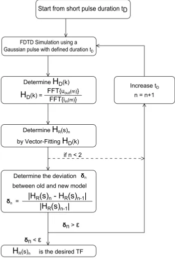
The proposed method can now be illustrated by the block diagram which is shown in Fig. 1. Starting from a compar-atively short excitation pulse, the desired observable is ob-tained from a numerical time-domain calculation. This al-lows to calculate the desired transfer functionHD(k)and a corresponding macromodel which is expressed byHR(s). A problem that is associated to the use of short pulses is that the discrete Fourier transform of such a signal will tend to have a sparse set of samples in the low frequency range. Due to dominant quasistationary contributions of typical light-ning currents, the main frequency range of interest is actu-ally located within this sparsely populated range of low fre-quencies. However, the sparsity makes the determination of a related transfer function susceptible to numerical errors. Therefore it is necessary to check the stability of results by using longer excitation pulses. It is then possible to compare the transfer functionsHR(s)that are obtained by excitation pulses of different lengths. If an increase of pulse duration does not lead to a significant change ofHR(s)it is assumed that the desired transfer function is obtained with sufficient accuracy.

To make the notion of a short excitation pulse more pre-cise, in Fig. 2 a standard double exponential lightning pulse of the form

FDTD Simulation using a Gaussian pulse with defined duration tD

Determine

H

H

FFT{uout(m)}

FFT{iin(m)}

Determine

H

by Vector-Fitting

H

Determine the deviation

between old and new model

δ_n = |HR(s)n - HR(s)n-1|

is the desired TF

H

Increase tD

if n < 2

n = n+1

|HR(s)n-1|

δ_{n > ε}

δ_{n <} ε

Start from short pulse duration tD

δ_n

Fig. 1. Block diagram of the proposed adaptive macromodelling routine.

i(t )=I0(e−αt−e−βt) (3)

is contrasted to a unipolar Gaussian pulse of the form

i(t )=I1·e −(t−t0)2

2·T2 . (4)

0 20 40 60 80 100 0

50 100 150 200

Time [us]

Amplitude [kA]

Double−Exp. Pulse Gaussian Pulse

Fig. 2. Graphical comparison between a double exponential pulse and a Gaussian pulse. Both pulses have the same maximum value and are characterized by a similar rise rime. The double expo-nential pulse is a standard pulse, defined within the standard (SAE 5412A, 2005), where the time from beginning to peak value 200 kA is 6.4 us, the time from beginning to decay to 50 percent peak value, that is 100 kA, is 69 us.

102 104 106

−100 −50 0 50

Frequency [Hz]

Amplitude density [dBA/Hz]

Gaussian Pulse

Double−Exp. Pulse

Fig. 3. Amplitude spectrum of both double exponential pulse and Gaussian pulse, as displayed in Fig. 2.

The duration of a Gaussian excitation is determined by the parameterT that is introduced in Eq. (4). It is inversely pro-portional to the frequencyFmaxwhich is defined as the

fre-quency where the amplitude spectrum of the Gaussian pulse has decayed by -20 dB if compared to its maximum value,

T∼ 1

Fmax

. (5)

Therefore a longer pulse duration implies a smaller value for Fmax and vice versa. This circumstance is illustrated

in Fig. 4 where Gaussian pulses corresponding toFmax=

0 1 2 3 4

0 0.2 0.4 0.6 0.8 1

Time [us]

1 MHz 3 MHz 10 MHz

Fig. 4. Gaussian pulses corresponding toFmax=1 MHz, 3 MHz, and 10 MHz. A larger value ofFmaximplies a shorter pulse dura-tion.

104 105 106

−65 −60 −55 −50 −45 −40 −35 −30 −25 −20

X: 3e+006 Y: −44.87

Frequency [Hz]

Amplitude Density [dBA/Hz]

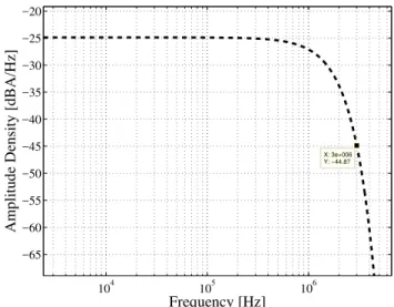
Fig. 5. Amplitude spectrum of a Gaussian pulse with Fmax=

3 MHz. At 3 MHz its value has decayed by 20 dB if compared to the maximum value.

1 MHz, 3 MHz, and 10 MHz are displayed. Additionally, the amplitude spectrum of the Gaussian pulse withFmax=

3 MHz is shown in Fig. 5.

It is suggested to use Gaussian excitations of different parametersFmax, corresponding to different time durations,

Fig. 6.Canonical tank geometry with interior tank pipe. For better visibility the front side of the tank is removed. The outer metallic frame serves as a return conductor.

Fig. 7. Enlarged view of tank pipe and circular exit hole. The arrows between tank pipe and boundary of the circular hole indi-cate voltage monitors which record the voltagevout(t )during the numerical simulation.

3 Numerical example: LEMP transfer function of a canonical tank model

As a specific example a canonical tank model is considered. The tank model consists of a rectangular box which contains a fuel pipe. The fuel pipe is electrically bonded to one side of the interior of the tank and leaves the tank through a circular hole as shown in Fig. 6. The tank is subject to a lightning current sourceiin(t )and the induced voltagevout(t )between

the fuel pipe and the boundary of the circular hole is the ob-servable of interest, compare Fig. 7 . Then a LEMP transfer function is defined according to Eq. (1).

The tank model has been created within the CST Mi-crowave Studio software which also is used to run the sim-ulation model and to generate the time domain datavout(t )

from the input variableiin(t )by means of the Finite

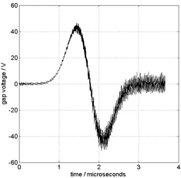
Integra-tion Technique (Clemens and Weiland, 2001). The result of a sample calculation is shown in Figs. 8 and 9. A mainly in-ductive response is observed, where voltage and current ap-proximately are related byu(t )=Ldi(t )_dt . This observation has been discussed in more detail in (Gronwald, 2010). As

Fig. 8.Sample Gaussian current excitationi_in(t ).

Fig. 9. Induced voltagevout(t )which is due to the current excitation of Fig. 8.

YR(s)= 1

R+s·L=

1_/L

s+R_/L,HR(s)

N=1

= r

s−p (6)

as an appropriate first order macromodel for the (inverse) transfer function of the canonical tank model. For details on macromodels of elementary networks it is referred to (An-tonini, 2003).

To calculate the parameters L and R which, according to (6), determine the LEMP transfer admittanceYR(s), it is first necessary to perform a time domain calculation for a given excitationiin(t )to compute vout(t ). Then the

corre-sponding discrete transfer functionHD(k)can be obtained from (1). Next, the inverse of this transfer function is fit-ted by means of the vector fitting method to the first order macromodelYR(s)which is given by (6). This yields the polepand residuerwhich both determine the parametersL

andR.

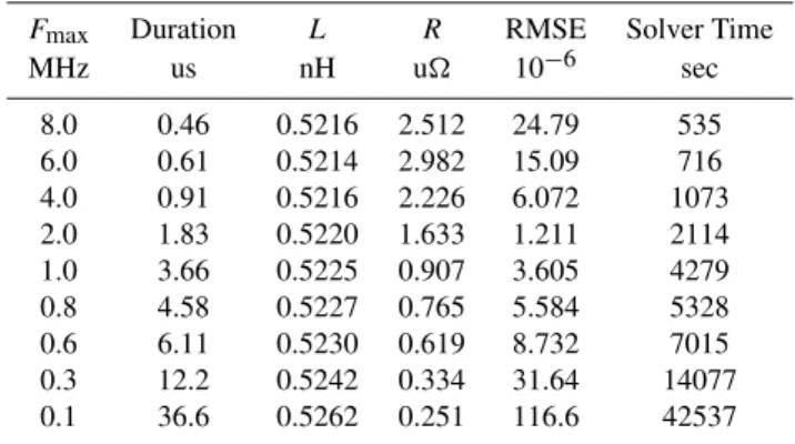
Following the procedure described in the previous para-graph, macromodels for the LEMP transfer function of the canonical tank model have been obtained for nine different Gaussian excitations. The results are given in Tab. 1. The chosen pulse durations vary by a factor of 80, that is, the computation times to computevoutvary by a factor of about

80 as well. The computations were performed on a single PC with 3.0 GHz CPU, 4 GB RAM, using the CST Microwave Studio 2010 software on a 32-bit Windows platform.

In order to judge the resulting parameters L andR one should note that the material of the tank model is mod-elled as highly conducting aluminium (σ=3.72·107S/m). Therefore the voltage response is dominantly inductive, such that the resistive response is somewhat hidden and does not significantly contribute to the voltage response. To judge the quality of the fitted macromodels the relative root mean square error is included in Tab. 1 which quantifies the de-viation between the numerically calculated transfer function

H_D−1(k)and the fitted first order LEMP transfer admittance

YR(s). It is seen that this deviation is small, thus justifying the assumption of a simple first order macromodel. Towards shorter pulse durations the fit error increases. This indicates that the possibility to shorten the pulse duration is limited due to numerical inaccuracies that accompany the computation of the Fourier transformation in order to obtainH_D−1(k). How-ever, the fit error increases towards longer pulse durations as well. To explain this observation it is noted that for long computation times numerical instabilities tend to build up, at least for the present numerical model which only contains minor losses. The smallest fit error occurs for the Gaussian pulse of time duration 1.83 us.

For further validation, it is of interest to compare the re-sults that were obtained from the Gaussian excitations to an analogous calculation using a standard double exponential pulse as displayed in Fig. 2. However, as it turns out, the long pulse duration leads to strong oscillations that are inter-preted as numerical instabilities and make it not feasible to

Table 1. Resulting macromodels for various Gaussian excitation pulses of different durations.

Fmax Duration L R RMSE Solver Time

MHz us nH u 10−6 sec

8.0 0.46 0.5216 2.512 24.79 535

6.0 0.61 0.5214 2.982 15.09 716

4.0 0.91 0.5216 2.226 6.072 1073 2.0 1.83 0.5220 1.633 1.211 2114 1.0 3.66 0.5225 0.907 3.605 4279 0.8 4.58 0.5227 0.765 5.584 5328 0.6 6.11 0.5230 0.619 8.732 7015 0.3 12.2 0.5242 0.334 31.64 14077 0.1 36.6 0.5262 0.251 116.6 42537

extract a meaningful LEMP transfer function. As an alter-native, an independent calculation was performed using the Method of Moment code CONCEPT-II which is defined in frequency domain (Brüns et al., 2011). To this end, a surface discretized model of the canonical tank was created and sim-ulations at 161 discrete frequency samples between 1 kHz and 8 MHz were performed. From the resulting data a corre-sponding first order macromodel was obtained with parame-tersL=0.5192 nH,R=2.8887 u, and a relative root mean square error RMSE=0.0023, thus supporting the results of Tab. 1.

4 Conclusions

Standard lightning pulses are characterized by durations of tenths of microseconds, thus leading to long computation times for time domain calculations of lightning current in-duced quantities. However, in order to obtain LEMP transfer functions it is also possible to use shorter excitation pulses, involving less computation time. Typically, LEMP transfer functions are characterized by only a small number of pa-rameters. Therefore the vector fitting procedure is useful to obtain these parameters which, in turn, can be used to quan-titatively compare transfer functions that are obtained from different excitation pulses. This makes it possible to quantify whether a short excitation pulse is sufficient to determine a LEMP transfer function with sufficient accuracy.

References

Apra, M., D’Amore, M., Gigliotti, K., Sarto, M. S. and Volpi, V.: Lightning Indirect Effects Certification of a Transport Aircraft by Numerical Simulation, IEEE Trans. Electromagn. Compat., 50(3), 513–523, 2008.

Brüns, H.-D., Freiberg, A., and Singer, H.: CONCEPT-II Man-ual of the Program System, (Hamburg University of Technology, February 2011), see also http://www.tet.tu-harburg.de/concept/, 2011.

Clemens, M. and Weiland, T.: Discrete electromagnetism with the finite integration technique, Progress In Electromagnetics Re-search, PIER, 32), 65–87, 2001.

Deschrijver, D., Pissoort, D., and Dhaene, T.: Adaptive Stopping Criterion for Fast Time Domain Characterization of Microwave Components, IEEE Microw. Wireless Compon. Lett., 19(12), 765–767, 2009.

Fisher, F. A., Perala, R. A., and Plumer, J. A.: Lightning Protec-tion of Aircraft, (Lightning Technologies, Inc., Pittsfield, USA), 1990.

Gronwald, F.: Classification and quantification of lightning-current induced voltages within aircraft structures, Proc. of the 9th Int. Symp. on EMC, EMC Europe 2010, Wroclaw, Poland, 559–564, 13–17 September, 2010.

Gustavsen, B. and Semlyen, A.: Rational Approximation of Fre-quency Domain Responses by Vector Fitting, IEEE Trans. Power Delivery, 14(3), 1052–1061, 1999.

Gustavsen, B.: Improving the Pole Relocating Properties of Vector Fitting, IEEE Trans. Power Delivery, 21(3), 1587–1592, 2006. Hoffman, J. D.: Numerical Methods for Engineers and Scientists,

2nd ed., (Marcel Dekker Inc., New York), 2001.

Lee, K. S. H. (ed.): EMP Interaction: Principles, Techniques, and Reference Data, revised printing, Taylor & Francis, Washington D.C. 1995.