E. Demirov , N. Pinardi , C. Fratianni , M. Tonani , L. Giacomelli , and P. De Mey
1Instituto Nazionale di Geofisica e Vulcanologia, Rome, Italy 2Bologna University, Corso di Scienze Ambientali, Ravenna, Italy 3LEGOS, Toulouse, France
Received: 12 December 2001 – Revised: 11 June 2002 – Accepted: 8 July 2002
Abstract. This paper describes the operational implementa-tion of the data assimilaimplementa-tion scheme for the Mediterranean Forecasting System Pilot Project (MFSPP). The assimilation scheme, System for Ocean Forecast and Analysis (SOFA), is a reduced order Optimal Interpolation (OI) scheme. The order reduction is achieved by projection of the state vec-tor into vertical Empirical Orthogonal Functions (EOF). The data assimilated are Sea Level Anomaly (SLA) and temper-ature profiles from Expandable Bathy Termographs (XBT). The data collection, quality control, assimilation and forecast procedures are all done in Near Real Time (NRT). The OI is used intermittently with an assimilation cycle of one week so that an analysis is produced once a week. The forecast is then done for ten days following the analysis day.
The root mean square (RMS) between the model forecast and the analysis (the forecast RMS) is below 0.7◦C in the sur-face layers and below 0.2◦C in the layers deeper than 200 m
for all the ten forecast days. The RMS between forecast and initial condition (persistence RMS) is higher than forecast RMS after the first day. This means that the model improves forecast with respect to persistence. The calculation of the misfit between the forecast and the satellite data suggests that the model solution represents well the main space and time variability of the SLA except for a relatively short pe-riod of three – four weeks during the summer when the data show a fast transition between the cyclonic winter and anti-cyclonic summer regimes. This occurs in the surface layers that are not corrected by our assimilation scheme hypothesis. On the basis of the forecast skill scores analysis, conclusions are drawn about future improvements.
Key words. Oceanography; general (marginal and semi-enclosed seas; numerical modeling; ocean prediction)
1 Introduction
One major goal of the Mediterranean Forecasting System Pilot Project (MFSPP, Pinardi et al., 2003) was to
demon-Correspondence to:E. Demirov ([email protected])
strate the feasibility of operational predictions of the baro-clinic basin scale circulation. Following the scientific plan of the project (see Pinardi and Flemming, 1998), a 10 days fore-casting system of currents, temperature and salinity fields was set up starting from 4 January 2000. The forecasting system includes three major elements: a data collection net-work, the general circulation model and the data assimila-tion scheme. Presently, this forecasting system produces a weekly ten days basin scale forecast, which is published on a perpetual Web site (http://www.cineca.it/mfspp). In the fu-ture, the operational forecasting activities will also include downscaling towards the shelf areas with nested models and ecological forecasting (Pinardi et al., 2002); the basin scale forecasts will provide the initial and boundary conditions for higher resolution nested shelf model forecasts.
The main elements of the basin scale forecasting system are reviewed in detail in different papers. The observing system is described in Manzella et al. (2001) for the Volun-tary Observing Ship (VOS), and Le Traon and Ogor (1998) for the satellite data. The ocean general circulation model (OGCM) of the basin scale forecasting system is presented in Demirov and Pinardi (2002). The data assimilation scheme is described and tested with a Mediterranean Sea circulation model by De Mey and Benkiran (2002) for satellite altimeter data and twin experiments XBTs.
In the present paper we describe the operational imple-mentation of the data assimilation scheme in a multivariate mode, never tried before, and we analyze the skill of the forecast with respect to observations and analyses for a six month period during the Targeted Operational Period of MF-SPP. This paper includes two main results: (a) the description of the method of assimilation of both SLA and XBT with one week assimilation cycle and (b) the evaluation of the forecast performance.
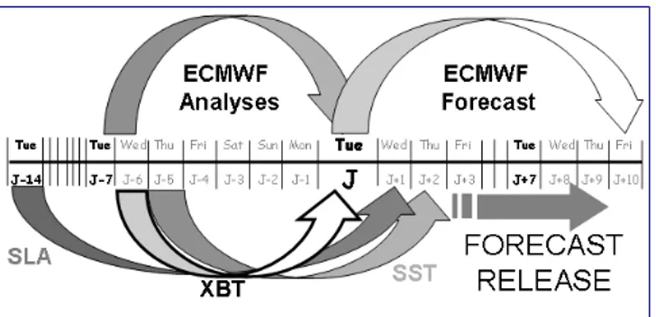
Fig. 1.Schematic NRT data collection system in MFSPP containing both oceanic and atmospheric data. The starting day of the forecast is indicated byJ. Each week the system is repeated. Forecast is released Friday with three days delay.
circulation and water mass variability known from observa-tions. However, there are still uncertainties in the model for-mulation that could produce incorrect forecasts. Between them, the relatively coarse resolution of the model in some areas (for instance in the Straits), uncertain subgrid scale physics parameterizations and rather modest spatial and tem-poral resolution of the surface forcing fields (half a degree and every six hours), could produce inaccuracies in the ini-tial conditions for the forecasts.
The predictability limit is strongly dependent upon the quality of the nowcast that in turn depends on the observing system and the data assimilation scheme. Thus the devel-opment of an optimal system that assimilates the NRT ob-servations was a major step during MFSPP. The assimilation scheme first of all should have been multivariate both in in-put and outin-put: the entering data are SLA and XBT profiles, but the corrections to the model first guess will be done on temperature, salinity and stream function, i.e. the baroclinic and barotropic components of the dynamical fields.
Last but not least, the forecast should be evaluated with respect to consistency, quality and accuracy (Murphy, 1993). This means that the predicted fields are objectively and sub-jectively compared to observations or analyses, trying to find out if and how much the model is capable of reproducing re-ality, how important is the data distribution and quality for the forecast, etc. The quality and accuracy is mainly given in terms of skill scores of various nature, already used in the meteorological literature (Murphy, 1988), and previous ocean forecasts (Walstad and Robinson, 1990).
The paper is organized in the following way. Section 2 discusses the data acquisition and organization of the forecast cycle. Section 3 presents the assimilation scheme. Section 4 discusses the results in terms of skill scores. Finally, Sect. 5 presents the conclusions.
2 The data acquisition and forecast cycle
The nowcast – forecast procedure of MFSPP is shown in Fig. 1. Since 4 January 2000 the MFSPP forecast is
pro-duced weekly with starting timeJ, which is Tuesday at noon of every week. The preparation and run of the forecast is done on several stages. Firstly, all data needed for the as-similation procedure and surface forcing calculation are col-lected. The procedure of data collection and quality check is briefly described in Appendix A. When the ocean satel-lite and insitu data and ECMWF analyses for the past 14 days are collected, the MFSPP nowcast/forecast procedure is run for the past 14 days to produce the model initial condi-tion for the starting dayJ of the forecast. The organization of the analysis run is related to the specific features of the MFSPP data assimilation scheme and is described in detail in the next paragraph. When the model initial condition for dayJ is calculated, the forecast run is done for 10 days for-ward. The ocean general circulation model (OGCM), used in the analysis and forecast runs is described in Appendix B.
The ocean and atmospheric data used in the analysis and forecast are collected on the dayJ+1 (the Wednesday of ev-ery week), except the SST field, which only becomes avail-able on the dayJ +2 (or Thursday of every week). Then the computational procedure requires between 6–10 h CPU time for the analysis and 1.5 h for the forecast. The CPU time for the analysis depends on the amount of assimilated ocean data, which can vary from one week to another. The forecast and analysis fields are published on the Web every Friday afternoon, i.e. with about 3 days delay after the start-ing day (J) of the forecast. This delay is mainly due to the time needed for processing the ocean SST data. Presently, the satellite SST data become available onJ +1 (Wednes-day), which makes it possible to run the forecast with only two days delay, i.e. now the forecast becomes available on Thursday of every week.
3 The Data assimilation scheme
The data assimilation scheme used in MFSPP is the Sys-tem for Ocean Forecasting and Analysis (SOFA). The main definitions, notations and a brief description of the scheme are presented in Appendix C. A more detailed discussion of SOFA can be found in De Mey and Benkiran (2002).
SOFA is a reduced order multivariate optimal interpola-tion scheme. The order reducinterpola-tion is achieved by projecting the state vector onto vertical EOFs which are the eigenvectors of the error covariance matrix for the forecast. The scheme is multivariate in terms of data input and corrections made on the model solution. Our particular state vector contains the model predictive variables such as temperature, salin-ity and barotropic stream function. The existence of dom-inant EOFs’ for the Mediterranean temperatusalinity re-lationship is discussed and demonstrated in Sparnocchia et al. (2003). Here, as in many other operational schemes, we use EOFs deduced from data rather than from an analysis of the forecast error covariance matrix.
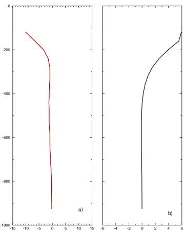
sur-Fig. 2.Bivariate Empirical Orthogonal Functions used in assimila-tion of SLA:(a)Temperature EOF,(b)Salinity EOF.
face altimeter information, i.e. the surface quasigeostrophic stream function at different depths, and then initialize the forecasts. On the basis of this experience, the order reduc-tion operator of SOFA is used here with vertical EOFs that this time are multivariate.
The observations do not need to be model dynamical vari-ables but they should be directly related to the model state variables. For this reason, an observation operator,H, is used to convert from model variables to measured variables for the case of SLA. We compute sea level with the full diag-nostic surface pressure formulation described by Pinardi et al. (1995) but we leave a simplifiedHoperator in the defi-nition ofKROOI, as explained in Appendix C. In particular, Hcontains only the geostrophic part of the signal and it as-sumes that bottom topography-related processes do not con-tribute to the signal. It is equivalent to the computation of dy-namic height with respect to a deep reference level with the addition of the barotropic mode from the model. Thus the operatorSHT projects the SLA into the temperature, salin-ity and stream function modes that are consistent with the geostrophic constraint for the SLA.
In the MFSPP assimilation system we used two different sets of EOFs, one for the XBT and the other for the SLA as-similation. This is done in order to strengthen the formal re-quirement that the observation operater projection on the null space of the Kalman matrix (Appendix C) is marginal and that the vertical EOFs should have a relatively high signature
on the observations. We believe that the same set of EOFs cannot fulfill the null space conditions for the both SLA and XBT, since SLA contains information mainly about theT , S
variability below the mixed layer while XBT give the mixed layer temperature. We use two different sets of order reduc-tion EOFs based upon our a priori knowledge of the informa-tion content of each observainforma-tional data set.
To assimilate SLA only one multivariate EOF for the whole basin was used, similarly to the scheme described in De Mey and Benkiran (2002). The SLA EOF is three-variate, i.e. computed from the covariance of temperature, salinity and stream function. The temperature and salinity compo-nents of the SLA EOF are shown in Fig. 2. The EOF extends only from 120 m downward. This choice of EOF for SLA is dictated from the past experience that showed that very few vertical modes can represent most of the dynamic height variability (Faucher et al., 2002) and that the SLA physically represents most of the geostrophic variability signal below the mixed layer. The choice of 120 m for the Mediterranean may be excessive but we took the conservative view of using EOFs that were already shown to be working in the region.
In order to assimilate the XBT data set, including the sur-face layer, a second set of bi-variate temperature and salinity EOFs was used. The EOFs were computed from an historical data set of the Mediterranean (Sparnocchia et al., 2003) in 9 different regions, chosen on the basis of the data coverage and known regional dynamical regimes. The EOFs retained only the variance around the seasonal signal and thus they vary every three months (winter consists of January, Febru-ary and March, spring of April, May and June, summer of July, August, September and autumn of October, Novem-ber and DecemNovem-ber). For each region, 10 dominant EOFs were considered. The transition between different regions was provided by a smooth change of the background error covariance matrix while the transition from one season to the next was sudden.
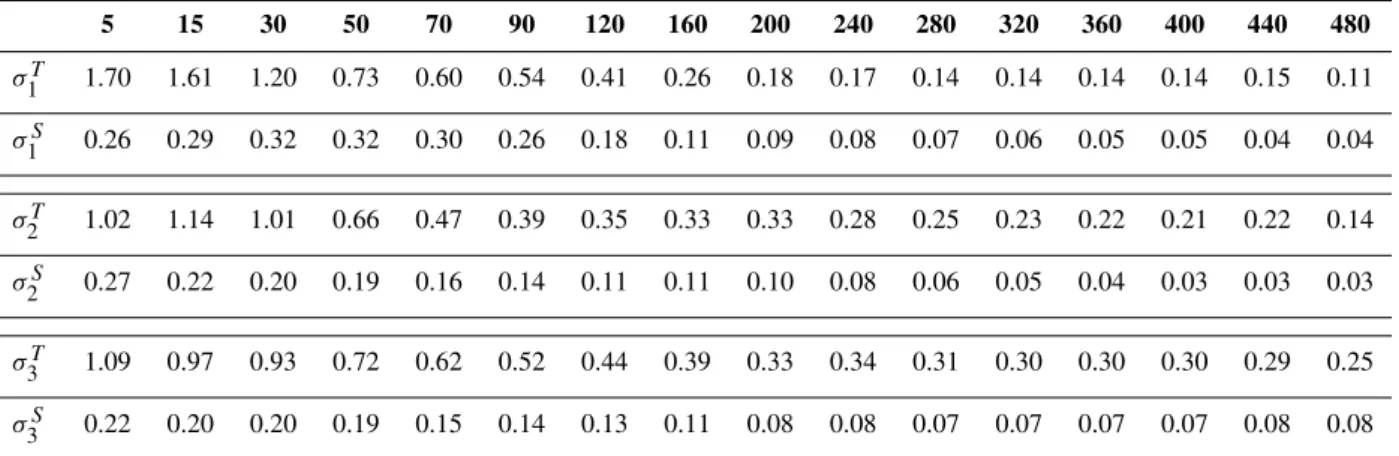
Table 2. The variance of temperature (◦C) and salinity (psu) at different depths for the 480 m surface layer in three different areas of the Mediterranean Sea: the Algerian Basin (σ1T, σ1S); the Tyrrhenian Sea (σ2T, σ2S); the Ionian Sea (σ3T, σ3S). The depth of model levels in the first line of the table is given in meters
5 15 30 50 70 90 120 160 200 240 280 320 360 400 440 480
σ1T 1.70 1.61 1.20 0.73 0.60 0.54 0.41 0.26 0.18 0.17 0.14 0.14 0.14 0.14 0.15 0.11 σ1S 0.26 0.29 0.32 0.32 0.30 0.26 0.18 0.11 0.09 0.08 0.07 0.06 0.05 0.05 0.04 0.04
σ2T 1.02 1.14 1.01 0.66 0.47 0.39 0.35 0.33 0.33 0.28 0.25 0.23 0.22 0.21 0.22 0.14 σ2S 0.27 0.22 0.20 0.19 0.16 0.14 0.11 0.11 0.10 0.08 0.06 0.05 0.04 0.03 0.03 0.03
σ3T 1.09 0.97 0.93 0.72 0.62 0.52 0.44 0.39 0.33 0.34 0.31 0.30 0.30 0.30 0.29 0.25 σ3S 0.22 0.20 0.20 0.19 0.15 0.14 0.13 0.11 0.08 0.08 0.07 0.07 0.07 0.07 0.08 0.08
Fig. 3. Bivariate Empirical Orthogonal Functions used in assimilation of XBT in (a) Algerian Basin, (b) Tyrrhenian Sea and(c)Ionian Sea. The continu-ous line shows the first EOF, the long dashed line the second EOF and the short dash line, the third EOF. The tem-perature EOFs are present in the upper panels and salinity EOFs in the bottom panels.
modes in these regions have maxima at intermediate depths between 100 and 300 m. The first bi-variate EOF in the Io-nian sea, Fig. 3c, show relatively low vertical variability sim-ilar to the dominant EOFs in most other Eastern
(b)
Fig. 4.The scheme of sequential assimilation of SLA and XBT data
(a)in the nowcast-forecast procedure and(b)in the analysis.
Sea. When composing theSmatrix, the EOFs are multiplied by the variance of the temperature and salinity at each level (see Table 2).
It is interesting to note that the first (dominant) EOFs in the Algerian and Tyrrhenian Sea have a structure below 120 m similar to that of the EOF used in SLA assimilation but this is not the case for the Ionian Sea. In fact, as explained by Sparnocchia et al. (2003), the EOFs are very different in the western and eastern Mediterranean basins, accounting for the different water mass variability in the two sub-basins.
The SLA and XBT sets of EOFs are used in a sequential procedure that ensures the combined assimilation of SLA and XBT with the different sets of EOFs (Fig. 4). The assimila-tion cycle is chosen to be a week, consistent with the XBT data distribution (Manzella et al., 2001) and the SLA data availability (Pinardi et al., 2003).
The first sequential procedure is callednowcast-forecast and it prepares each week the initial condition for the fore-cast (Fig. 4a). Every assimilation cycle, two sequential runs are made – the first with assimilation of one of the data sets in smoother mode and the second with the other data set as-similated in filter mode. The multivariate EOFs forψ, T,
S are used for assimilation of SLA and the bi-variate T , S
EOFs are used for assimilation of XBT profiles. This way each data set is projected into its optimal vertical modes, and contributes to the estimate of the nowcast. The SLA assim-ilation is applied only in regions deeper than 1000 m. This assumption is based upon the surface dynamic height
com-Fig. 5.Mean climatology of the sea surface height in meters, com-puted from 1993–1997 model simulations.
putation studies of ¨Ozsoy et al. (1993) who showed that a deep reference level (zero motion assumption) would gener-ate more realistic surface currents and sea level variability. The model SLA is then calculated by subtracting the model mean sea surface level that is shown in Fig. 5. This field was computed from a model simulation of the Mediterranean cir-culation from 1993 to 1997 to be consistent with the mean subtracted from the observed SLA.
The second procedure is calledanalysisand it is presented in Fig. 4b. It uses only the results of the smoother assimila-tion mode for both SLA and XBT. This means that we pro-duce an optimal estimate of the circulation once every week with the usage of both past and future observations. Between one analysis and the other we run the model with surface meteorological analyses, thus producing the best dynamical extrapolation between successive optimal ocean state esti-mates. The daily data set formed by this analysis/simulation is called, collectively, the analysis data set, even if the ocean data are inserted only once a week. In both procedures of analysis and nowcast-forecast, the model surface fluxes are not only calculated from the analysis atmospheric fields but are also corrected with the observed weekly mean SST using Eq. (B1).
4 Forecast skill scores
Our study period goes from 4 April 2000 to 31 October 2000. It coincides with the first period of operational forecasting in MFSPP and it was chosen because it has the largest data density for both in situ and satellite data. In the following the model forecast is checked against observations and analyses following the Murphy (1993) definition of indices for “good” forecast. These are:
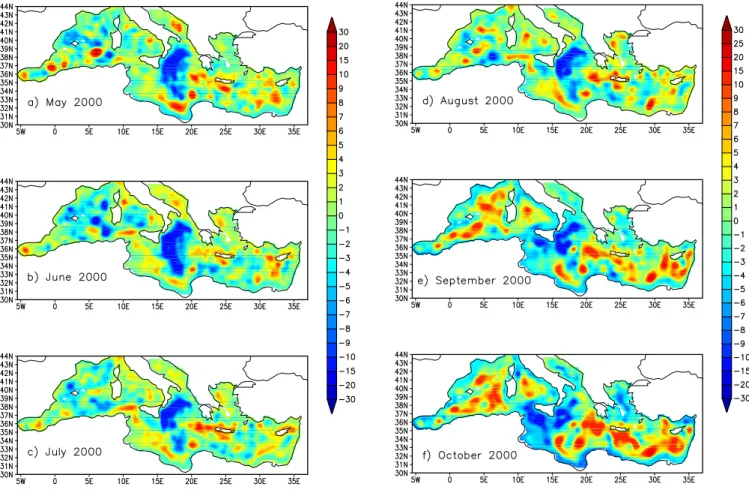
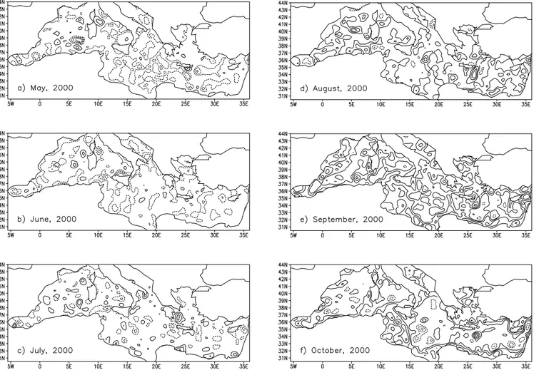
Fig. 6.Monthly mean of MFSPP SLA analysis in cm for(a)May 2000,(b)June 2000,(c)July 2000,(d)August 2000,(e)September 2000,
(f)October 2000.
2. Quality: the objective correspondence between analy-ses and forecasts using statistical indices to quantify the level of discrepancy between forecast and analyses. 3. Accuracy: the objective correspondence between
obser-vations and analysis using statistical indices to quantify the analysis error with respect to the data.
4. Value: the benefits realized by the users of the forecast. The value of the Mediterranean forecasts cannot be yet quantified since the user basis of the forecasts is still very limited. The other indices will be discussed in the sections below.
4.1 Consistency
Our consistency check is defined on the basis of the compar-ison between satellite data and analysis for SLA. Instead of using along-track values of SLA from the model and obser-vations, we will compare the analyses done with two differ-ent analysis systems. The first is based only on the statistical knowledge of the satellite data structure and is explained by Le Traon et al. (1998). The observed SLA is mapped by ob-jective analysis (OA) techniques using three weeks data to estimate a field every week. The weekly OA field is then
av-eraged to produce monthly mean distributions of SLA for the period May–October 2000. The second field is produced by the MFSPP analysis system of Fig. 4b, and its monthly mean distributions for the same period of time are shown in Fig. 6. The correspondence between MFSPP SLA analysis and OA SLA data is evaluated by the differences of corresponding fields (Fig. 7).
Both data and model show relatively strong cyclonic cir-culation (or low, negative values of SLA) all over the basin during the May–June period. Anticyclonic eddies and gyres are locally intensified in the Algerian Basin, Southern Io-nian, Peloponnesus and south-east of Crete, the so-called Iera-Petra gyre area, and the Shikmona gyre area (south of Cyprus). These features are quasi-permanent and they are observed with variable intensity during the whole period. The large cyclonic anomaly in the Ionian Sea is very inter-esting; this is maintained both in the model and data for the whole period (Figs. 6 and 7). Anticyclonic anomalies are stronger in the model than in the data during the May–June period (Figs. 7a and b) since the difference fields are mainly negative.
Fig. 7.Difference between monthly mean OA SLA computed only from satellite observations (see the text) and monthly mean of MFSPP SLA analysis for(a)May 2000,(b)June 2000,(c)July 2000,(d)August 2000,(e)September 2000,(f)October 2000. The contour interval is 5 cm and the 0 isoline is not plotted.
intensification). The strongest change in the observed data, which, hereafter, will be referred to as the summer transition of SLA, appears in July and August. The observed SLA val-ues reach the highest positive valval-ues during September 2000. The MFSPP analyses are not capturing this summer SLA transition, which can be seen by the positive heigh values of the difference between data and model analysis in July and August (Figs. 7d and e). There are two major differences between the satellite data and the MFSPP SLA analysis in this period. Firstly the change in the SLA analysis field is smoother with a gradual increase of the positive values. The highest values of SLA in the model solution are observed in October 2000 (Fig. 6). Secondly, the anticyclonic intensifi-cation in the analysis solution appears only in the deep areas like Algerian – Provencal basin, Ionian Sea and the Levan-tine Basin. In the shallow areas of the Strait of Sicily, the Aegean and the Adriatic Sea the values of model SLA re-main relatively low during the whole period after the sum-mer transition (Figs. 7d–f). As we mentioned in the Sect. 4, the SLA assimilation is done only in the deeper parts of the basin (deeper than 1000 m). The data assimilation has an
im-portant impact on the model solution there, which even with some delay develops circulation structures equivalent to that in the observations. In the shallow areas however, where no SLA data assimilation is done, the summer transition is not captured at all by the model dynamics.
Fig. 8.Root mean square temperature forecast error at(a)5 m;(b)
30 m;(c)280 m; and(d)400 m. Different curves correspond to 31 different 10-day forecasts carried out from April to October 2000.
4.2 Quality
The rms error between two quantities,φf andφr in general
is defined as:
rms(φ)= v u u t1
N
N
X
1
(φf −φr)2 (1)
whereN is the number of data used in the evaluation. Here we will useφf for the forecast fields andφr for the analysis
or observations.
Figure 8 shows the root mean square (rms) error between temperature forecast and analysis for 31, ten days forecasts carried out between 4 April and 31 October 2000. The pa-rameter plotted on Fig. 8 will be referred hereafter as forecast rms temperature error.
The forecast rms temperature error in the surface layer (5 m) increases almost linearly with time. This is mainly due to errors in the atmospheric forcing computed with ECMWF forecast surface fields. We remind that the analysis is done
Fig. 9. Root mean square temperature forecast (red line) and per-sistence (blue line) errors at(a)5 m;(b)30 m;(c)280 m and(d)
400 m for the 31, 10-day forecasts carried out from April to October 2000.
not only with a more accurate representation of surface forc-ing, calculated using the atmospheric analysis fields, but it uses the heat flux correction with observed SST. The error in the estimation of the surface heat flux during the forecast influences the thermal structure in the whole surface mixed layer in a coherent way and in fact, at 30 m depth, the fore-cast rms temperature error behaves almost linearly, as at the surface.
Below the surface layer, the forecast rms temperature error grows relevantly only at the analysis time, i.e. at the end of every assimilation cycle (or every 7th day). In Fig. 8 we see in fact that at depth the forecast rms temperature error increases relevantly only at day 7 when new data are inserted at depth.
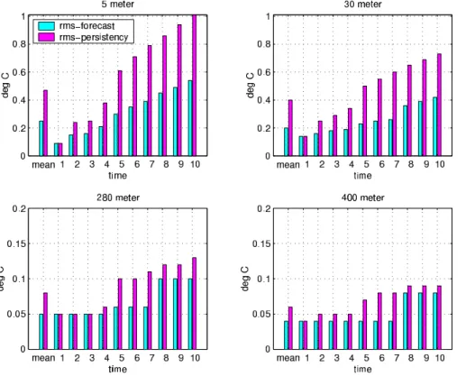
Fig. 10.Average root mean square tem-perature forecast (blue bars) and persis-tence (red bars) errors at(a)5 m;(b)30 m;(c)280 m and(d)400 m. The aver-age is carried out over the 31 forecasts done from April to October 2000.
0.7◦C, and below 200 m, between 0.03◦C–0.18◦C. The same forecast rms temperature error is shown on Fig. 9 together with the rms error between forecast and initial condition. Hereφr is taken to be the nowcast for each week; the skill
score computed this way will be referred to hereafter as per-sistence rms temperature error. With very few exceptions, the forecast rms temperature error is less than the persistence rms temperature error during the whole forecasting period and at every model depth. In the surface layer, where the time variability is the highest, the persistence rms temper-ature error during the spring and summer can reach values close to 1.2◦C, i.e. almost twice the maximum forecast rms temperature error at this level.
The rms forecast and persistence errors are minimal at the beginning of every assimilation cycle with values which de-pend on the differences in the initial conditions of forecast and analysis. The latter are computed with data assimilation in the smoother mode while the forecast uses the nowcast produced with a combination of smoother and filter schemes. During the assimilation cycle, the rms persistence error in-creases due to the dynamical evolution of the model fields. At the surface, the rms persistence error is relatively high during the period of strong heating in May and June, while at 30 m the highest rms persistence error is present during July– August, i.e. after the formation of the seasonal thermocline. The rms forecast error in the surface layers is mainly due to the uncertainty in the surface forcing but it always remains below the rms persistence error.
At 280 and 400 m (Figs. 9c and d) the changes in the rms forecast and persistence errors are relatively high at the
be-ginning of every assimilation cycle. During the rest of the time their variability is relatively small. The forecast and persistence rms errors, after April, reveal a bi-weekly vari-ability which is related to the combined assimilation cycle of SLA and XBT data. After the beginning of July, the bi-weekly variability of the forecast and persistence rms errors become different. This is due to the fact that the regular XBT data collection stopped and the main assimilated data set was composed of SLA observations. The analysis and the now-casts were produced with a relatively small amount of XBT data or just as model simulations, since the XBT data were not available.
The mean value of forecast and persistence rms temper-ature error for the period April–October 2000 is shown in Fig. 10 for different model depths. The forecast rms tempera-ture error is highest at the surface, where it reaches 0.55◦C at the last forecast day. Its mean value decreases with the depth. Its mean is about 0.2◦C at 30 m and less than 0.05◦C at 280
and 400 m. The maximum of the persistence rms tempera-ture error in the surface layer is about 1◦C while at 30 m it is about 0.68◦C. The mean value of the persistence rms tem-perature error has values of 0.45◦C at the surface and 0.38◦C at 30 m. At all depths it is higher than the forecast rms error. Another statistical parameter, which characterize the fore-cast quality is the anomaly correlation, which is defined as follows:
Ca=
PN
n=1(Tna−Tnca)(T f
n −Tncf)
q PN
n=1(Tna−Tnca)2
q PN
n=1(T f
n −Tncf)2
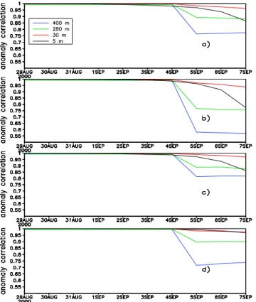
Fig. 11. Anomaly correlation (Eq. 2) of forecast and analysis for
(a)the whole Mediterranean Sea; (b)the Algerian Basin; (c)the Tyrrhenian Basin;(d)the Ionian Sea. The black curves correspond to the 5 m depth, the red to 30 m, the green to 280 m and the blue to 400 m.
whereTaandTf are the analysis and forecast temperature fields, respectively,Tca is the climatology computed from the analysis, Tcf is the forecast climatology and N is the number of the model grid points for each region or the whole basin.
The temperature anomaly correlation is shown for the whole basin in Fig. 11a, for the Algerian Basin in Fig. 11b, for the Tyrrhenian Sea in Fig. 11c and for the Ionian Sea in Fig. 11d. The anomaly correlation in the surface layer re-mains relatively high during the first 7 days. However, due to the new observations inserted in the analysis at day 7, the correlation falls down to 0.8–0.6 in the last three days of the forecast period. Our choice of climatology makes the terms in Eq. (2) insensitive to the changes occurring during the first seven days of forecast. In the future, a more sensitive skill score index for correlation should be used.
4.3 Accuracy
The forecast and persistence rms temperature errors and the anomaly correlations are measures of the departures of fore-cast from the analyses, i.e. the best estimate of the ocean state computed by using model and data. A different way to evaluate the quality of the forecast is to compare the model solution directly to the observations. Since the amount of in-dependent data (not used in the analysis) for the period
con-sidered is limited, we use here the assimilated data itself be-fore they are inserted in the model. Thus we compare the model simulation done with an analysis initial condition and atmospheric fields to the observations.
During the assimilation procedures, a misfit is calculated, that is the difference between model simulation and the ob-servations at the time and locations of the obob-servations. The model simulation is given at the observation location using a simple linear interpolation scheme. The rms statistics are then calculated on such misfits. We define the normalized mean square (nms) as:
nms= PN
i=1(φm−φo)2
PN i=1φ2o
, (3)
whereφmis the model field,φo the observation andN, the
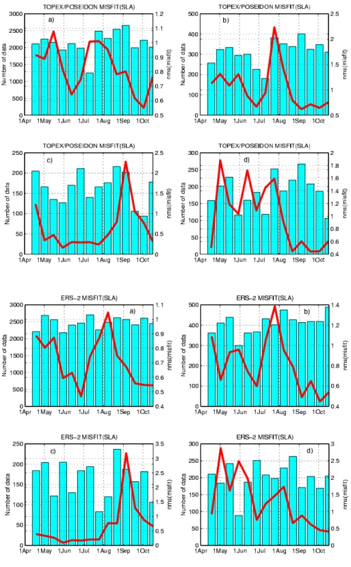
number of observations used in the weekly analysis scheme. In Figs. 12 and 13 the nms for SLA is shown for Topex/Poseidon and ERS-2 data, respectively. Both figures show a decrease of nms from April to June/July in the whole basin and the Algerian and Tyrrhenian. However, nms grows back again in August for the Algerian Basin and in Septem-ber for the Tyrrhenian Sea. In addition, in the Ionian, the nms remains relatively high up to August–September. This is the problem of the missed summer SLA transition period discussed above. It is interesting to note that, during the pe-riod May–August (Fig. 6) when the SLA show the presence of anticyclonic eddies in the Ionia, the nms is the highest. In contrast, during September–October, the strong intensifi-cation of the quasi-permanent anticyclonic gyres such as the Iera-Petra, the Mersa-Matruh and the gyres in the Shikmona area is relatively well represented also by the model solution and the nms decreases. In the Tyrrhenian Sea, it cannot re-produce the anticyclonic intensification occurring in Septem-ber.
In summary, the nms of the SLA misfit shows that the model can capture, with different skills, different parts of the ocean variability. It shows problems for capturing the intense mesoscale activity, presumably due to the coarse resolution of the model which is just eddy permitting but not resolv-ing. Different regions have different rates of decrease of the nms misfit but they show a growth of errors in the period of anticyclonic intensification. Another important point is that the value of the nms is different between the two data sets, hinting that T/P is closer to the model solution than ERS-2.
The rms temperature misfit for the XBT data, calculated with Eq. (1) is shown in Figs. 14 and 15 for two different model levels, 5 and 360 m, respectively. The zero values cor-respond to the periods of no XBT data. In the surface layer of the whole basin (Fig. 14a) the misfit varies between 0.4◦C and 0.7◦C. The error increases during the end of spring and beginning of summer. The maximum errors is about 0.7◦C in the Algerian Basin (Fig. 14b) for the first week of June, about 0.55◦C in the Tyrrhenian Sea (Fig. 14c) for the first week of May and about 0.7◦C in the Ionian Sea (Fig. 14d) for the first week of July.
Fig. 12. Normalized root mean square misfit of SLA (Eq. 3) computed for Topex – Poseidon data for (a)whole basin; (b) Algerian Basin;(c) Tyrrhe-nian Sea;(d)Ionian Sea. The blue bars indicate the number of SLA observa-tions available during every bi-weekly analysis cycle.
Fig. 13. Normalized root mean square misfit of SLA (Eq. 3) computed for ERS-2 data for(a)whole basin;(b) Al-gerian Basin; (c)Tyrrhenian Sea; (d)
Ionian Sea. The blue bars indicate the number of SLA observations available during every bi-weekly analysis cycle.
The variability of the error is relatively low in the intermedi-ate layers of the Algerian Basin (Fig. 15b) and the Tyrrhenian Sea (Fig. 15c), where it changes between 0.2◦C and 0.3◦C. In
the Ionian Sea the rms temperature misfit error in the middle of April is about 0.9◦C and decreases to 0.3◦C.
From the rms temperature misfit error it is possible to de-duce that, with two weeks repeat sampling, the error has time to approximately double or triple but is is still kept on
reason-able values, below 1◦C. Toward the end of the XBT sampling experiment, in July, the 5 m rms temperature misfit error in-creases due to the decreasing number of observations. Below the threshold of 50–60 XBT every two weeks, the error starts to double in most of the regions (Figs. 14a, b and d).
Fig. 14. Normalized root mean square misfit between forecast and XBT obser-vations at 5 m depth for(a)whole basin;
(b)Algerian Basin;(c)Tyrrhenian Sea;
(d)Ionian Sea. The blue bars indicate the number of XBT profiles available during every bi-weekly analysis cycle.
Fig. 15. Normalized root mean square difference between forecast and XBT observations at 400 m depth for
(a) whole basin; (b) Algerian Basin;
(c) Tyrrhenian Sea; (d) Ionian Sea. The blue bars indicate the number of XBT profiles available during every bi-weekly analysis cycle.
solution close to the observations. These authors show that the time period during which the assimilated information is retained by the model is shorter than two weeks. In addition, the data used in Raicich and Rampazzo (2003) are synthetic XBT profiles regularly distributed in time while the XBT ob-servations, used in operational forecasts, were rather sparse in both time and space due to the irregularity of the realistic sampling scheme and the loss of data by the satellite
commu-nication system. Thus the highly variable number and posi-tion of the XBT data used in forecast initializaposi-tion, as shown on Fig. 14, reduces their impact on the model solution and in-creases the model errors in accordance with the Raicich and Rampazzo (2003) results.
mer, when the surface heating is relatively strong. We have to mention that our vertical mixing parameterization does not include the contribution of some important processes like wind mixing. The heat flux correction is computed with the weekly mean SST. At the same time, the fast changes in the upper thermal structure of the sea during this period have a significant daily and day to day component which decreases the impact of the satellite SST corrections.
The maxima of temperature misfit at intermediate depths is about 0.6◦C for the whole basin (see Fig. 15) which is higher than the value (about 0.12◦C) of rms forecast error (Fig. 8). This indicates that the data assimilation is only partly capa-ble of correcting the differences between the observed in situ values and model parameters. This may be due to several reasons, the first being the possible inconsistency between SLA and XBT assimilation schemes at depth.
5 Conclusions
In this paper we presented the methodology of data assimila-tion developed for the MFSPP operaassimila-tional forecasting exer-cise lasting from April to October 2000. The basic assimila-tion scheme is SOFA that is an OI multivariate reduced order technique that uses vertical EOFs to reduce the order of the assimilation problem.
The method successfully assimilates a combination of SLA and XBT profiles and uses weekly SST to correct for heat fluxes during analysis cycles. For the first time, a multi-variate OI scheme has been used to assimilate SLA and XBT observations that form the basis of the NRT ocean monitor-ing programs in the world’s ocean’s and now in the Mediter-ranean Sea. The OI is used with different sets of EOF in order to optimize the process of information extraction from these two data sets.
The vertical multivariate EOF used for SLA assimilation corrects the subsurface temperature, salinity and barotropic stream function fields. A single EOF is used for SLA assimi-lation since it is known that most of the variability in dynamic height can be represented by very few vertical modes. The correction from SLA is done only below 100 m since, again, it is believed that the SLA signal is indicative of geostrophic dynamics below the mixed layer.
XBT are assimilated with a multivariate OI scheme. For this we use 13 different regions, 4 different seasons and 10 vertical bivariate EOF. This allows us to get the benefit of XBT assimilation throughout the first 500 m of the water column where most of the XBT are collected. Such a large
surface parameters to force the ocean forecasts for ten days. Finally the consistency, quality and accuracy of the fore-cast has been evaluated with respect to observations and anal-yses.
The forecast rms temperature error versus persistence rms temperature error shows that for a six months period, from April to October 2000, forecast always beats persistence. The forecast rms temperature error is maximum at the sur-face, reaching 0.6◦C after ten days and lower in the subsur-face, up to 0.3◦C after the same ten days. The anomaly cor-relation drops to about 0.75–0.8 after ten days, only in the subsurface. We are tempted to deduce that the predictability time of the large-scale temperature field is longer than ten days at all levels in the Mediterranean, given the observing system network implemented during MFSPP. Coastal areas however, remain still with high consistency errors between analyses and observations and in the future the forecasting system should develop the scheme to use multivariate assim-ilation of SLA also in these areas.
The nms error of the SLA misfit show that the model can sometimes reproduce the mesoscale, some other times the larger scale subbasin scale gyre variability. However, the assimilation system proposed here shows problems to accu-rately retain information from the SLA during rapid transi-tion periods, such as the July–August period in year 2000. More detailed regional analysis (not shown here) showed that in different regions this summer SLA transition lasted only 3-4 weeks. Under such conditions, the weekly assimilation of SLA is not efficient enough to “keep” the model close to the data. A possible way to improve the model forecast is to use smaller data assimilation cycles with more frequent insertion of data.
The future forecasting system for the Mediterranean Sea should consist of all three main components described here. While satellite data will be continuously available, the VOS-XBT may be more sporadic in the future but nevertheless still necessary to correct the subsurface temperature in a re-alistic way. Thus recommendations are that subsurface data acquisition programs will be sustained, perhaps with the help of more advanced technologies, such as ARGO subsurface floats and advanced multiparametric VOS system. On the other hand, the data assimilation scheme should be improved in order to accommodate the model error covariance matrix that allows us to consider assimilation of SLA into shallower areas.
System Pilot Project”.
The Editor-in-Chief thanks a referee for his help in evaluating this paper.
Appendix A Near real time data collection and quality control
The data collected weekly for the MFSPP forecasting ac-tivities include NRT observations used in the data assimi-lation procedure and meteorological ECMWF analysis and forecast surface fields used in the computation of the sur-face forcing for the OGCM. The NRT observations consist of: (a) satellite data for sea surface temperature (SST) and sea level anomaly (SLA); (b) vertical temperature profiles by Expandable BathyTermograph (XBT) collected along the 7 VOS routes described by Manzella et al. (2001). The mete-orological parameters used in the MFSPP forecast are: mean sea level pressure, total cloud cover, zonal and meridional wind components at 10 m, temperature at 2 m and dew point temperature at 2 m. In this section we describe briefly the data collection and preprocessing procedures for the differ-ent data sets.
The SST data are collected in the Centre de Meteorologie Spatiale (CMS) of Meteo France, Toulouse and the Istituto di Fisica dell’Atmosfera of the CNR in Rome. The data are obtained from the night orbits of the NOAA-AVHRR-14 and the NOAA-AVHRR-15 satellite sensors. The final SST data set is a weekly mean (centered on every Monday) and con-sists of data interpolated on the Mediterranean Sea OGCM grid (with resolution 18◦ × 18◦) using an objective analysis method (see Buongiorno-Nardelli et al., 2003).
The along track Topex-Poseidon (T/P) and ERS - 2 satel-lite data for SLA are collected and analyzed at the Collec-tion and LocalizaCollec-tion Satellitaire (CLS) located in Toulouse, France. The data are corrected first for the orbit error, com-puted by using a local inverse method (Le Traon and Ogor, 1998). Then SLA values are computed by subtracting a 5-year mean of T/P and ERS - 2 data form 1993 to 1997. The along – track correlated errors are corrected by application of a local adjustment method using simultaneous T/P and ERS2 data over a period J0-22 to J0-2 days where J0 is consid-ered to beJ +1 on Fig. 1. This local adjustment diminishes the residual error due to orbit and inverse barometer effects which are subtracted from the sea level signal. Smoothing cubic splines are then used to estimate a bias for each point along the track and to produce corrected along-track SLA observations.
The XBT data are collected along seven tracks with an along-track spatial nominal resolution of 12 nm (Manzella et al., 2001). Each track was repeated once per month from September 1999 until December 1999 and twice per month from January until June 2000 (with the exception of the track crossing longitudinally all the basin that was made only once a month). The temperature profiles have a vertical resolution of 0.6 m and reach the maximum depth of 460 m or 760 m (depending upon T6 or T7 probes being used). Decimated
data are received in NRT and consist of temperature observa-tions at 15 vertical levels. They are transmitted on the Global Teleconnection System (GTS) and also collected at ENEA – La Spezia, Italy, where a first quality control is made before the data are provided on a free ftp site. At the forecasting center, and before the data are used in the assimilation pro-cedure, a quality control check is carried out on each XBT profile through a graphical visualization of the vertical pro-file and a check on the position.
The ECMWF meteorological data are provided by Meteo France, Toulouse, France, for the basin scale forecast system with 12 h delay, i.e. on Wednesday of each week. Before starting the forecast procedure a quality control of the data is done by a graphical visualization of the fields.
Appendix B The model
The model used is based upon the Modular Ocean Model (MOM), adapted to the Mediterranean Sea by Roussenov et al. (1995) and Korres et al. (2000). The model grid has 31 vertical levels, and an horizontal resolution of18◦×18◦. Hori-zontal turbulent mixing is biharmonic with tracer coefficients equal to 1.5×10¹⁰m4s−1and momentum coefficients equal to 5×10⁹m4s−1. Vertical turbulent coefficients are constant and equal to 0.3 10−4m2s−1for tracers and 1.5 10−4m2s−1 for momentum. A convective adjustment procedure (Cox, 1984) is applied in statically unstable areas of the water col-umn with 10 repeat cycles maximum each time step. This choice of physical mixing was elaborated in the articles cited above. Even if simple, it is capable of reproducing the bulk of water mass variability when it is associated with high fre-quency atmospheric forcing (Castellari et al., 2000). The transport through the Strait of Gibraltar is parameterized by extending the model area westward of Gibraltar to a longi-tude 9.25◦W. In this model area, which is a part of the North Atlantic, between latitudes 33◦30′N≤ φ ≤ 37◦N, the sur-face forcing is switched off and temperature and salinity are relaxed toward annual mean climatological fields.
The model is rigid lid but a diagnostic computation of sea level is done at each time step following Pinardi et al. (1995). The sea level is proportional to the surface pressure on the rigid lid due to large scale dynamical response of the sea level to internal dynamics and surface forcing, excluding ex-ternal gravity waves, atmospheric surface pressure response and tidal sea level changes.
whereT is the model surface temperature,SST is the weekly observed field interpolated to the model time step between the previous week value and the present week and the nudg-ing constant is equal toλ = 1.67 m/day. The sea surface water flux is parameterized only with a salt flux given by the relaxation of model sea surface salinity toward a new cli-matology, called MED6 (Brankart and Pinardi, 2001). The relaxation constant is everywhere 2 m/day.
The model is initialized with a 7-year model experiment, forced with perpetual monthly mean forcing (a repeating sea-sonal cycle). The model is then run from 1 January 1997 to 1 September 1999 with surface forcing computed from ECMWF 6-h analyses. From 1 September 1999 to 4 January 2000 the model is run only with assimilation of XBT and SST heat flux correction. Then the MFSPP operational fore-cast period started 4 January 2000. From 4 April 2000 the combined assimilation of SLA and XBT was inserted into the operational forecasting procedure.
Appendix C SOFA algorithm
C.1 Optimal interpolation
Let us define the state vector xn as a vector formed by model state variables at the n-th model time step. Then the vector
xfn+1=M xan
(C1) is the model forecast, whereMis the model, xan is the an-alyzed estimate of the state vector at n-th time step. The vector of the observationsyois related to the true statextby the equality:
yo=H xt+ǫ (C2)
whereǫis the observational error andHis the observation operator. NormallyHis a linear interpolation of model state variables into observational positions. In addition to that, Hmay be more complex as explained in Appendix C.2 for satellite SLA. The forecast error covariance matrix is defined by:
Bfn=Eh(xfn−xnt)(xfn−xtn)Ti (C3) whereE denotes the expectation operator. The analysis at each time step is computed as follows
xan=xfn+K
yo−H(xfn)
(C4)
our caseCis multivariate and contains cross correlations be-tweenT , Sandψ, and also correlations between model state variables in horizontal and vertical directions. In the MFSPP data assimilation schemeDfwas assumed to vary seasonally as explained later. The OI gain is defined as:
KOI=BfnHTHBfnHT+R
−1
(C6) whereRis the data error covariance matrix.
SOFA is a reduced order multivariate optimal interpola-tion scheme. The order reducinterpola-tion is achieved by project-ing the state vector into vertical EOFs which compose the columns of the S matrix, the simplification operator. The vertical EOFs are the eigenfunctions of theBfnmatrix which is now written:
Bfn=STBfrS (C7)
whereBfr contains the horizontal correlations of the n mul-tivariate EOF modes defined in S. Inserting Eq. (C7) into Eq. (C6) we obtain:
K=S−1BrfHrTHrBrfHrT+Rr−1 (C8) whereHr=HSTand the matrixRr takes into account the representativity error in the reduced space.
Now Eq. (C6) can be rewritten as:
KOI=S−1KROOI (C9)
where
KROOI=BrfHrTHrBrfHrT+Rr−1 (C10) The order reduction procedure considers a limited number of vertical EOFs that should, however, still be representative of the error covariance matrix.
C.2 Observational operator for the sea level anomaly
The observation operator for the sea level anomaly is cal-culated on the basis of the work of Pinardi et al. (1995). In addition to the linear interpolation, in this case it repre-sents the combination of model state variables necessary to compute the observed SLA. In our case,Hcontains only the geostrophic contribution to SLA, i.e.:
η= f ψ gH0
− 1
ρ0H0
Z 0 −H0
where the assumption is that the depthH0is constant,ψis
the barotropic stream function,ρ0is the reference density,ρ
is the density,g– the gravity andf – the Coriolis parameter. In our case SLA assimilation is applied for the regions deeper than 1000 m. Correspondingly the parameterH0is set equal
to 1000 m.
References
Angelucci, M. G., Pinardi, N., and Castellari, S.: Air-sea fluxes from operational analysis fields: intercomparison between ECMWF and NCEP analysis over the Mediterranean area. Phys. Chem. Earth, 23, 569–574, 1998.
Bignami, F., Marullo, S., Santoleri, R., and Schiano, M. E.: Long wave radiation budget in the Mediterranean Sea, J. Geophys. Res., 100, 2501–2514, 1995.
Brankart, J.-M. and Pinardi, N.: Abrupt cooling of the Mediter-ranean Levantine Intermediate water at the beginning of the eighties: observational evidence and model simulation, J. Phys. Oceanogr., 31, 8, 2, 2307–2320, 2001.
Buongiorno-Nardelli, B., Larnicol, G., D’Acunzo, E., Santoleri, R., and Le Traon, P. Y.: Near real time SLA and SST products during 2-years of MFS pilot project: processing, analysis of the variabil-ity and of coupled patterns, Ann. Geophysicae, this issue, 2003. Castellari, S., Pinardi, N., and Leaman, K. D.: A model study of
air-sea interactions in the Mediterranean Sea, J. Mar. Syst. 18, 89–114, 1998.
Castellari, S., Pinardi, N., and Leaman, K.: Simulation of water mass formation processes in the Mediterranean Sea: Influence of the time frequency of the atmospheric forcing, J. Geophys. Res., 105, 10, 24 157–24 181, 2000.
Cox, M.: A primitive equation, 3-dimensional model of the ocean. GFDL Ocean Group Tech. Rep. 1, Geophys. Fluid Dyn. Lab., Princeton, N. J., pp. 43, 1984.
Daley, R.: Atmospheric Data Analysis, Cambridge University Press, Cambridge, U.K., pp. 471, 1991.
De Mey, P. and Benkiran, M.: A multivariate reduced-order optimal interpolation method and its application to the Mediterranean basin-scale circulation, In: Ocean forecasting, (Eds) Pinardi, N. and Woods, J., Springer Verlag, 281–306, 2002.
De Mey, P. and Robinson, A.: Assimilation of altimetry data eddy fields in a limited-area quasi-geostrophic model, J. Phys. Oceanogr., 17, 2279–2293, 1987.
Demirov, E. and Pinardi, N.: Simulation of the Mediterranean Sea circulation from 1979 to 1993. Part I: The interannual variability, J. Mar. Syst., 33/34, 23–50, 2002.
Faucher, P., Gavart, M., and De Mey, P.: Isopycnal EOFs in the North and Tropical Atlantic and their use in estimation problems, J. Geophys. Res., submitted, 2002.
Hellerman, S. and Rosenstein, M.: Normal monthly wind stress over the world ocean with error estimates, J. Phys. Oceanogr, 23, 1009–1039, 1983.
Kondo, J.: Air-sea bulk transfer coefficients in diabatic conditions, Boundary Layer Meteorol., 9, 91–112, 1975.
Korres, G., Pinardi, N., and Lascaratos, A.: The ocean response to low frequency interannual atmospheric variability in the Mediter-ranean Sea. Part I: Sensitivity experiments and energy analysis,
J. Climate, 13, 705–731, 2000.
Le Traon, P. Y., Nadal, F., and Ducet, N.: An improved mapping Method of multisatellite altimeter data, J. Atmos. Oceanic Tech., 15, 522–533, 1998.
Le Traon, P. Y. and Ogor, F.: ERS-1/2 orbit improvement using Topex/Poseidon: the 2 cm challenge, J. Geophys. Res., 103, 8045–8050, 1998.
Manzella, G. M. R., Gardin, V., Cruzado, A., Fusco, G., Gacic, M., Galli, C., Gasparini, G. P., Gervais, T., Kovacevic, V., Millot, C., Petit DeLaVilleon, L., Spaggiari, G., Tonani, M., Tziavos, C., and Velasquez, Z.: EU-sponsored effort improves monitoring of circulation variability in the Mediterranean, EOS Trans., AGU, 82, 43, 497–504, 2001.
Murphy, A. H.: Skill score based on the mean square error and their relation to the correlation coefficient, Monthly Weather Review, 116, 2417–2424, 1988.
Murphy, A. H.: What is a good forecast? An essay on the nature of goodness in weather forecasting, Weather Forecasting, 8, 281– 293, 1993.
¨
Ozsoy, E., Hecht, A., ¨Unl¨uata, ¨U., Brenner, S., Sur, S., Bishop, H. I., Latif, M. A., Rozentroub, Z., and Oˇguz, T.: A synthesis of the Levantine Basin circulation and hydrography, 1985–1990, in: Physical oceanography of the Eastern Mediterranean Sea, (Eds) Robinson, A. R. and Malanotte-Rizzoli P., Deep-Sea Res., Part II, 40, 1075–1119, 1993.
Pinardi, N., Rosati, A., and Pacanowski, R. C.: The sea surface pressure formulation of rigid lid models. Implications for alti-metric data assimilation, J. Marine Systems, 6, 109–119, 1995. Pinardi, N. and Flemming, N.: The Mediterranean Forecasting
Sys-tem Science Plan, EuroGOOS Publication No. 11, Southampton Oceanographic Center, Southampton, 1998.
Pinardi, N., Auclair, F., Cesarini, C., Demirov, E., Fonda-Umani, S., Giani, M., Montanari, G., Oddo, P., Tonani, M., and Zavatatareli, M.: Toward marine environmental predictions in the Mediter-ranean Sea coastal areas: a monitoring approach, in: Ocean fore-casting, (Eds) Pinardi, N. and Woods, J., Springer Verlag., 339– 376, 2002.
Pinardi, N., Allen, I., Demirov, E., De Mey, P., Korres, G., Las-caratos, A., Le Traon, P. Y., Maillard, C., and Manzella G. M. R.: The Mediterranean Ocean Forecasting System: First phase of implementation (1998–2000), Ann. Geophysicae, this issue, 2003.
Raicich, F. and Rampazzo, A.: Observing System Simulation Ex-periments for the assessment of temperature sampling in the Mediterranean Sea, Ann. Geophysicae, this issue, 2003. Reed, R. K.: On estimation insolation over the ocean, Progr.
Oceanogr, 17, 854–871, 1977.
Roussenov, V., Stanev, E., Artale, V., and Pinardi, N.: A seasonal model of the Mediterranean Sea circulation, J. Geophys. Res., 100, 13 515–13 538, 1995.
Sparnocchia, S., Pinardi, N., and Demirov, E.: Multivariate Em-pirical Orthogonal Function analysis of the upper thermocline structure of the Mediterranean Sea from observations and model simulations, Ann. Geophysicae, this issue, 2003.