www.ocean-sci.net/7/629/2011/ doi:10.5194/os-7-629-2011
© Author(s) 2011. CC Attribution 3.0 License.
Ocean Science
Development of Black Sea nowcasting and forecasting system
G. K. Korotaev1, T. Oguz2, V. L. Dorofeyev1, S. G. Demyshev1, A. I. Kubryakov1, and Yu. B. Ratner1 1Marine Hydrophysical Institute National Academy of Sciences, Sevastopol, Ukraine
2Institute of Marine Sciences Middle East Technical University, Erdemli, Turkey Received: 1 March 2011 – Published in Ocean Sci. Discuss.: 27 April 2011
Revised: 9 September 2011 – Accepted: 15 September 2011 – Published: 11 October 2011
Abstract. The paper presents the development of the Black Sea community nowcasting and forecasting system under the Black Sea GOOS initiative and the EU framework projects ARENA, ASCABOS and ECOOP. One of the objectives of the Black Sea Global Ocean Observing System project is a promotion of the nowcasting and forecasting system of the Black Sea, in order to implement the operational oceanogra-phy in the Black Sea region. The first phase in the realization of this goal was the development of the pilot nowcasting and forecasting system of the Black Sea circulation in the frame-work of project ARENA funded by the EU. The ARENA project included the implementation of advanced modeling and data assimilation tools for near real time prediction. Fur-ther progress in development of the Black Sea nowcasting and forecasting system was made in the frame of ASCABOS project, which was targeted at strengthening the communi-cation system, ensuring flexible and operative infrastructure for data and information exchange between the Black Sea partners and end-users. The improvement of the system was made in the framework of the ECOOP project. As a result it was transformed into a real-time mode operational nowcast-ing and forecastnowcast-ing system. The paper provides the general description of the main parts of the system: circulation and ecosystem models, data assimilation approaches, the system architecture as well as their qualitative and quantitative cali-brations.
1 Introduction
The basis for operational oceanography is the observing sys-tem providing regular oceanographic data in real time mode. Operational observations together with modern computers,
Correspondence to:V. L. Dorofeyev (dorofeyev [email protected])
numerical models and data assimilation methods allow de-veloping the marine environment nowcasting and forecast-ing. Nowcasting and forecasting of marine environment is similar to the meteorological weather prediction. Integrat-ing structurally different sets of observations which are made available by satellite sensors, moorings, floats and ship-based measurements in the marine nowcasting and forecasting sys-tems allows continuous evolution of the ocean fields in a con-venient form with rather high accuracy.
The initiatives for setting up a Black Sea marine nowcast-ing and forecastnowcast-ing system under the umbrella of the Euro-pean Commission Framework programmes started with the FP5 ARENA project (A Regional Capacity Building and Networking Programme to Upgrade Monitoring and Fore-casting Activity in the Black Sea Basin) during the mid-2000s. It is further improved in the FP6 ASCABOS project (A Supporting Programme for Capacity Building in the Black Sea Region towards Operational Status of Oceano-graphic Services) and transformed into a real-time mode op-erational system in the ECOOP projects (European COastal-shelf sea Operational observing and forecasting system) dur-ing the second half of the 2000s. The overall goal of ECOOP was to consolidate, integrate and further develop existing Eu-ropean coastal and regional seas operational observing and forecasting systems into an integrated pan-European system. Different basin-scale models mainly resulted from MERSEA system provided initial and boundary conditions for the coastal forecasting. The Black Sea community nowcasting and forecasting system was essential part of the ECOOP. The development and operation system involved a partner-ship and collaborative efforts of various institutions from the Black Sea riparian states as they joined together in different groups for modelling, observations, data assimilation, data management and serving with limited financial resources. The present form of the Black Sea nowcasting and forecast-ing system offers a suite of interdisciplinary models and data assimilation schemes that are linked to regional atmospheric
model products, and observational sensors mounted on a va-riety of platforms.
A critical element of this remarkable achievement in a rather short time was a long history of scientific collabo-ration on the Black Sea oceanographic research. The cir-culation and ecosystem models were run simultaneously at Marine Hydrophysical Institute (MHI), Ukraine and Institute of Marine Sciences (IMS), Turkey. MHI was also responsi-ble for retrieving satellite data, their processing and assimila-tion into the models. The meteorological data were provided by the high resolution regional atmospheric model which is fully operational at National Meteorological Administra-tion (NMA) in Romania as a regional implementaAdministra-tion of the French global atmospheric model ALADIN. The input data to the oceanic models are collected through Internet or down-loaded from the data base management system. The model products were also stored by the data base management sys-tem at IMS. A back up syssys-tem exists in NIMRD (Romania) which was also responsible to disseminate the forecast prod-ucts and analyses data to the institutions such as Institute of Oceanology, Bulgarian Academy of Sciences (IO-BAS), Bulgaria, IGF (Georgia), NMA (Romania), Shirshov Insti-tute of Oceanology (SOI), Russia and MHI (Ukraine) to run their high-resolution sub-regional models.
The presented paper consists of the next main parts: de-scription of the Black Sea circulation models used in the nowcasting and forecasting system with schemes of data as-similation; the circulation model calibration; description and calibration of the biogeochemical model; and architecture of the Black Sea nowcasting and forecasting system.
2 Black Sea circulation models and data assimilation approach
Achievements of the operational oceanography during the last decade are considerably connected with significant im-provement of the ocean models skill, assimilation procedures (Agoshkov et al., 2010) and increase of computers power. Numerical models of the oceanic circulation and ecosystems (Zalesny et al., 2008; Zalesny and Tamsalu, 2009) can be op-erated now even on personal computers reproducing rather accurately the state of the marine environment and future changes according to the external forcing.
2.1 Description of the circulation models
The Black Sea general circulation models used by the now-casting and forenow-casting system are based on the finite-difference approximation of the primitive equations. One of the models is developed by MHI and it is written in the Cartesian coordinate system. The model uses z-coordinate in the vertical direction. It uses Philander – Pacanovsky (Pacanovsky and Philander, 1981) parameterisation of the vertical turbulent viscosity and diffusion. Another model is
the implementation of the Princeton Ocean Model (POM), that is also expressed in the Cartesian coordinates in the hor-izontal directions and terrain following sigma coordinate in the vertical. The Princeton University model has an advan-tage with respect to the former one in terms of its more so-phisticated parameterization of the turbulent viscosity and diffusion using the Mellor-Yamada 2.5 level turbulence clo-sure (Mellor and Yamada, 1982) that permits a more realistic representation of the surface mixed layer and the sub-surface cold intermediate layer. The horizontal currents, vertical ve-locity, temperature, salinity and turbulent diffusion coeffi-cients obtained by the POM are used to run the ecosystem model in an offline mode.
Both the MHI model and POM equations are discretized on the C-grid (Arakawa, 1966). The momentum equations in the MHI model are presented in Lamb form which conserves energy and potential enstrophy in the barotropic divergence-free case (Demyshev et al., 1992). The MHI model has 35 non-uniformly spaced levels which are compressed to-wards the free surface and the bottom. Horizontal grid resolution is 5 km in both directions that resolves well the mesoscale processes with the Rossby radius of deformation of about 20–25 km in deep part of the Black Sea (Dorofeyev et al., 2001). Leap-frog scheme is used for time discretiza-tion with periodical switch on of the Matsuno scheme to avoid time slipping feature of the Leapfrog scheme. Ver-tical coefficients of turbulent viscosity and diffusion were parameterised by Philander –Pakanovsky formula as it was suggested by Friedrich and St`anev (Friedrich and St`anev, 1988). Horizontal turbulent viscosity coefficient and diffu-sion coefficient were chosen constant and equal to 5×10⁷ and 5×105cm2s−1respectively.
POM has 7 km horizontal grid step and 26 sigma–levels, which are more frequently near the sea surface and near the bottom. An advantage of the POM model consists of more sophisticated parameterization of the vertical turbulent dif-fusion and viscosity coefficients. Therefore the results, ob-tained with the POM model, were used as input parameters for the Black Sea ecosystem model.
The surface and lateral boundary conditions of the mod-els are provided by the regional atmospheric model, and the climatic data for the river runoffs, water and salt transports through the Kerch and Bosphorus Straits. Surface forcing is an output of the ALADIN atmospheric model of National Meteorological Administration of Romania. ALADIN atmo-spheric model, the limited area version of the global spectral model ARPEGE/IFS of MeteoFrance, is a tool for the dy-namical adaptation and simulation of hydrostatic meso-scale phenomena. It has horizontal space resolution of 24 km and provides 54 h forecast for the Black Sea of wind stress, evap-oration and precipitation, sensitive and latent heat flux, long and short wave radiation every 6 h. Because the Black Sea is a semi-enclosed basin, the lateral boundary conditions are no-slip and zero heat and salt fluxes everywhere except the Bosphorus and Kerch Straits and some major rivers where
the temperature and salinity boundary conditions are specific at inflow conditions. Diffusive heat and salt fluxes are set to zero in the straits outflow points.
2.2 Data assimilation approach
Data assimilation is a procedure permitting to combine ob-servations with model simulations for adequate simulation of the marine environment real state (Ghil and Malanotte-Rizzoli, 1991). Operational Black Sea circulation model as-similates real-time satellite altimetry and sea surface temper-ature.
Sea level anomalies provided by AVISO service were con-verted into the sea level height (SSH) according to the al-gorithm described by Korotaev (Korotaev et al., 2001). It is then assimilated into the model using the optimal interpola-tion approach and permits to correct the simulated fields by observations. The correction is performed at the moment of observations and has the following form:
⌢
S(x,y,z,t )=S(x,y,z,t )+
N X
n=1
Wn·[ς (x¯ n,yn,t )−ς (xn,yn,t )] (1)
wherex,y,zare spatial coordinates,tis time,S(x,y,z,t )is any field which characterises the sea state (below we shall call it as salinity) and is predicted by the model to the mo-ment of observation,ς (x,y,z,t )is the sea level field which is predicted by the model,N is the number of observations of a fieldςandς (x,y,z,t )¯ is its observed value.⌢S(x,y,z,t )
is the optimal estimation of the fieldS(x,y,z,t ) that takes into account observations of the field ς (x,y,z,t ). Weight coefficientsWn are calculated through the cross-covariance
functionPSς of errors of salinitySand sea levelς forecast and the auto-covariance functionPς ςof errors of the field
ς(Knysh et al., 1996).
Let us present error covariance functions in the form
PSς(x,y,z,x′,y′,t )=σS(x,y,z,t )·σς(x′,y′,t )· ¯PSς(x,y,z,x′,y′,t ) (2) Pς ς(x,y,x′,y′,t )=σς(x,y,t )·σς(x′,y′,t )· ¯Pς ς(x,y,x′,y′,t )(3) whereσS(x,y,t )andσς(x,y,t )are standard deviations of errors of salinity and sea level predictions, respectively,P¯Sς
is the cross-correlation function of errors of the sea level and salinity fields andP¯ς ς is auto-correlation function of errors
of the sea level. Let the following assumptions:
1. Errors of the predicted fields are stationary in time as well as horizontally uniform and isotropic. Then
σS=σS(z) (4)
σς=const (5)
¯
PSς= ¯PSς(r,z) (6)
¯
Pς ς= ¯Pς ς(r) (7)
wherer2=(x−x′)2+(y−y′)2.
-0.06 -0.04 -0.02 0 0.02 0.04 0.06
500 400 300 200 100 0
cs(z)
ct(z)
Z
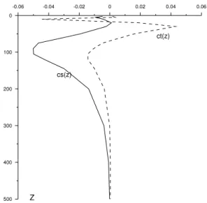
Fig. 1.Normalized weight coefficients for extrapolation of temper-ature and salinity with depth.
2. Cross-correlation between salinity and sea level is pre-sented as a product of two factors:
¯
PSς(r,z)= ¯PSς(r)· ¯PSς(z) (8)
3. A statistic of errors of the predicted fields is propor-tional to the natural statistics of the same fields. Under these assumptions, the variance, auto-correlation and cross- correlation functions estimated from obser-vations are used in the simulations. Normalized weight coefficients for the temperature and salinity fields are presented on Fig. 1.
Sea surface temperature (SST) retrieved from NOAA AVHRR data was assimilated in the model. Reception and pre-processing of AVHRR data was carried out by MHI group. SST retrieved from AVHRR measurements on 1 km grid was interpolated then on the model grid. The assimila-tion of SST derived from AVHRR sensors was carried out by replacing the simulated temperature within the upper mixed layer by the observed SST. The mixed layer depth was deter-mined by combining the simulated temperature and salinity profiles analysis and Obukhov’s formula (Obukhov, 1946), which follows from the turbulent energy balance. Bearing in mind that the cloudiness is impenetrable for IR radiation and some gaps can appear on SST maps derived from AVHRR data. Therefore, the observed SST is optimally interpolated using the SST prediction as a base. Then interpolated values are assimilated as it was explained above. Such approach permits to avoid artificial fronts on the simulated SST maps. SST and SSH assimilation permits to keep the surface layer thermodynamics and topography of permanent pycn-ocline close enough to the real state. However operational
observations in the Black Sea do not cover the deep layers of the basin with required density. Profiling floats observations are too rare and only special approach elaborated last time (Demyshev et al., 2010) should permit to assimilate them. Therefore the stratification of the basin is simulated by the model. The model is not perfect and after long enough inte-gration it slides to its own climate. Typical trends are about 0.05 degrees per year and 0.1 ppt per year in the permanent pycnocline. The model trends are not important for a short term forecast but it should be corrected when the model run is long enough. In our case we have initialized the model strat-ification in January 2005 and then it is simulated by model more than five years until the end of ECOOP and further in the framework of My Ocean project. Assimilation of the temperature and salinity profiles obtained by averaging of the climatic arrays over the basin area was used in the model which operated during ECOOP to avoid undesirable trends. This method has significant drawback as the climatic profiles are unable to trace decadal variability of vertical stratifica-tion. Nevertheless assimilation of the climatic profiles make possible to prevent slow sliding of the model to its own cli-mate.
3 Circulation model calibration
The circulation models have been subject to extensive set of qualitative and quantitative tests prior to the operational phase. Next two subsections present some of those tests to show the model ability to reproduce major characteristics of the Black Sea dynamics and important features of the tem-perature and salinity stratification.
3.1 Qualitative model calibration
The Black Sea is an elongated basin situated between 40◦56′ and 46◦33′N with the maximum dimension along the lon-gitude equal to 1148 km. The southern end of the Crimea peninsula and the north point of the Anatolian coast convex-ity determine the narrowest place of the Black Sea with the width about 260 km dividing the whole basin on eastern and western sub-basins. The Black Sea is deep enough. Its mean depth is about 1300 m and its maximal depth is more than 2200 m. A broad shelf with the depth of 0–100 m occupies the northwestern part of the sea where concentrated 80 % of the river fresh water discharge. All precipitation and half of river fresh water inflow are evaporated. The rest part of the Black Sea water outflows through the Bosphorus Strait. Wa-ter exchange through the Bosphorus Strait has a two-layer structure. The Marmara Sea water of higher salinity is trans-ported to the Black Sea along the bottom of the strait. Vol-ume transport of the upper flow (near 0.02 Sv) exceeds twice the lower one. Correspondingly, the salinity of the Marmara Sea is approximately twice higher than that on the surface of the Black Sea. Inflow of the salt water through the
Bospho-rus Strait determines the density stratification of the sea. The deep-sea salinity is near 22.5 ppt against 18–18.5 ppt on the surface. A well-pronounced permanent pycnocline is situ-ated on the depth of 150–300 m that makes internal Rossby radius be equal to 25 km.
Monthly-mean atmospheric circulation is of a cyclonic character above the Black Sea during the whole year. Pre-vailing of cyclones provides positive wind stress curl for the whole year with maximum in winter and minimum in sum-mer. The positive wind stress curl and the buoyancy contrast between the fresh river inflow and salt water supply through the Bosphorus Strait induce cyclonic circulation in the sea. A permanent feature of the upper layer circulation is the Rim Current, encircling the entire Black Sea and forming a large-scale cyclonic gyre. The Rim Current is located above the continental slope and has the width of 40–80 km. Direct ob-servations of current velocity from surface buoys show that the maximum speed of the stream is usually 40–50 cm s−1 increasing sometimes up to 80–100 cm s−1. The shape of the coastline probably conditions appearance of two smaller cy-clonic gyres in the western and the eastern parts of the basin. The Rim Current is concentrated above the shallow pycn-ocline and the volume transport by the current is estimated as 3–4 Sv. A general opinion is that shallow and sharp pycno-cline restricts propagation of seasonal signal from the surface and seasonal variability is concentrated in the upper 100 m. General cyclonic circulation induces the rise of the dynami-cal sea level toward the coast. Full range of spatial variability of the dynamical sea level depends on a season and changes from 25 to 40 cm so that the mean amplitude of the sea level spatial variability is about 15 cm (Blatov et al., 1984).
Large-scale hydrographic surveys, satellite observations and eddy-resolving numerical simulations show that the in-stantaneous surface currents differ from a simple gyre due to the strong mesoscale variability (Sur et all., 1994; Kortaev et al., 2003). Permanent and transient mesoscale anticyclones are observed at the right side from the jet. The most promi-nent feature is the anticyclonic eddy in the southeastern cor-ner of the basin. Strong meanders of the Rim Current and mesoscale eddies are formed near the Bosporus Strait and along the Anatolian coast. The area of the bottom slope be-tween the northwestern shelf and the deep part of the sea is also the region of the increased mesoscale variability resulted from the Rim Current meandering. The internal Rossby ra-dius, which is equal to 25 km, defines a typical length scale of mesoscale features. The mesoscale variability of the sea level may have the amplitude of 10–15 cm as the velocity of surface mesoscale currents achieves 50 cm s−1.
Surface geostrophic currents derived from altimetry (Ko-rotaev et al., 2001) manifest obviously annual cycle of the basin circulation. The Rim Current is the most intense in winter-spring seasons. Summer circulation attenuates sig-nificantly and in the autumn season the Rim Current usu-ally brakes on the set of mesoscale eddies. Simple explana-tion of the Black Sea seasonal cycle of circulaexplana-tion is done
28 30 32 34 36 38 40 41
42 43 44 45 46 47
17.04.2003
28 30 32 34 36 38 40
41 42 43 44 45 46 47
09.04.2003
28 30 32 34 36 38 40
41 42 43 44 45 46 47
03.05.2003
28 30 32 34 36 38 40
41 42 43 44 45 46 47
25.04.2003
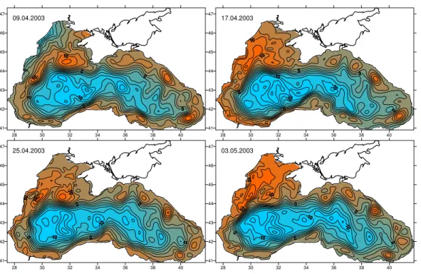
Fig. 2.Short-term evolution of the sea surface topography.
by (Korotaev et al., 2001, 2003). Increase of the cyclonic vorticity of the surface wind in January produces intensifica-tion of the upwelling on the bottom of Ekman layer, which induces the rise of pycnocline. The shallowest pycnocline observes a quarter of period (i.e. three months) later. How-ever, the rise of pycnolcline in the central part of the basin should be compensated by its deepening near the coast due to the conservation of the fluid volume. The deepening of pycnocline occurs above the continental slope where the on-shore velocity component breaks the geostrophyc balance. The displacement of the pycnocline near the coast is signif-icantly higher than its rise in the open sea as the volume of fluid replaced in the center of the basin should be preserved along the beach. Therefore, the slope of pycnocline toward the coast increases significantly at the beginning of spring. The intensity of the Rim Current, which is in geostrophic balance, is highest at the same time. The weakening of the wind stress curl in summer vice versa is accompanied by the deepening of pycnocline in the open sea ant its rise near the coast. The reduction of the pycnocline slope is manifested at the attenuation of the Rim Current.
The overall circulation system possesses a set of quasi-persistent anticyclonic eddies on the coastal side of the Rim Current zone (Kortaev et al., 2003). The most notable fea-tures include the Bosphorus, Batumi, Sukhumi, Caucasus, Kerch, Crimea, Sevastopol, Constantsa, and Kaliakra anticy-clones. The Bosphorus eddy is observed on the average for 260 days per year with a mean lifetime of about 85 days. The Batumi anticyclone forms in early March and lives usually
until the end of October. An average it is observed during 210 days per year. The Sukhumi eddy is manifested about 120 days per year and exists typically for about a month once it forms. It is mostly observed in autumn-early winter months after the collapse of the Batumi gyre. The Caucasus eddy ap-pears about 160 days per year starting at spring. The Kerch eddy is also one of the most pronounced features of the Black Sea eddy dynamics with an average persistence of 240 days and a mean lifetime of 80 days. The spring and autumn sea-sons are found to be more favoured periods for its presence. The Crimea anticyclone occurs mainly in August-September, and is observed around 115 days per year. The mean period for each event is about a month. The winter and summer are found to be most preferred periods for formation of the Sev-astopol eddy. It is observed for about 150 days per year and has the mean lifetime of 50 days. The Constantsa and Kali-akra anticyclones are observed for about 190 days per year with a typical lifetime of about 50 days.
A chain of eddies is observed also along the Anatolian coast but usually they have more intermittent character and travel slowly eastward along the coast. The Sakarya, Sinop and Kizilirmak eddies tend to exhibit more quasi-permanent character due to controls exerted by regional topographies.
The Black Sea circulation model was first calibrated by the climatological data. The attention was focused particu-larly on reproduction of the Black Sea Rim Current and its seasonal variability as well as main coastal anticyclonic ed-dies (e.g. Batumi gyre). Other specific features for the model calibration are the reproduction of the main halocline, the
28 30 32 34 36 38 40 41
42 43 44 45 46 47
25.04.2003
Fig. 3.Surface circulation in spring season simulated by the model.
seasonal thermocline, salinity decrease from the basin center to its periphery. It is necessary to evaluate the model possibil-ity to reproduce the cold intermediate layer (CIL), its repro-duction sites and two mechanisms of formation (e.g. winter convection in the central part of the basin and subduction of cold waters from the northwestern shelf).
An example of the Black Sea surface topography evolu-tion during April 2003 is shown on Fig. 2. The strong gra-dient around the periphery corresponds to the Rim Current jet, its contours are streamlines of the surface geostrophic currents; thus, closed contours represent mesoscale eddies. The overall circulation system shown in Fig. 2 therefore pos-sesses the meandering Rim Current system cyclonically en-circling the basin and a set of coastally-attached anticyclonic eddies around the basin, the most notable of which are the Bosphorus, Batumi, Sukhumi, Caucasus, Kerch, Sevastopol, and Constantsa anticyclonic eddies on the coastal side of the Rim Current zone. The Batumi anticyclone is present in the south-eastern corner of the basin as the most intense and per-sistent of the Black Sea coastal eddies. The Rim Current structure is shown also on Fig. 3.
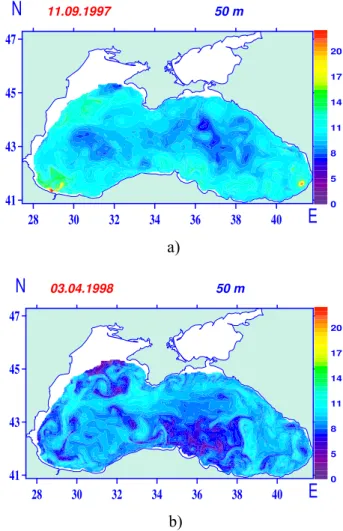
The maps of temperature distribution on the 50 m depth re-veal a complex picture of spatial variability caused by shear currents (Fig. 4). For example, Fig. 4a shows relatively warm and salty Mediterranean water injected by the Mediterranean underflow near the northern exit of the Bosphorus Strait and its subsequent distribution by currents. It appears to be an in-termittent feature depending on the character of large scale circulation features near the strait. Small lenses of warm water similar to “meddies” in the Atlantic Ocean near the Gibraltar strait are formed near the Bosphorus mouth and then transported by Rim current. Such warm lens is seen in Fig. 4a in the southeast corner of the basin. Such features have not been documented and yet to be confirmed by obser-vations.
Figure 4b shows subduction of cold waters (dark color) from the northwest shelf to the deep sea. In the same fig-ure the set mushroom-like structfig-ures also is visible near the
28 30 32 34 36 38 40
E
41 43 45 47
N
0 5 8 11 14 17 20 50 m
11.09.1997
a)
28 30 32 34 36 38 40
E
41 43 45 47
N
0 5 8 11 14 17 20 50 m
03.04.1998
b)
0 4 8 0 0 4
Fig. 4.Temperature distribution on the depth 50 m.
northwest shelf of the sea, in the southwestern corner of basin just opposite to a mouth of the Bosporus Strait and along the Anatolian coast. Usually such mushroom-like structures are observed on the sea surface on satellite images, but rarely captured by direct observations that require high resolution synoptic sampling at the right time and location.
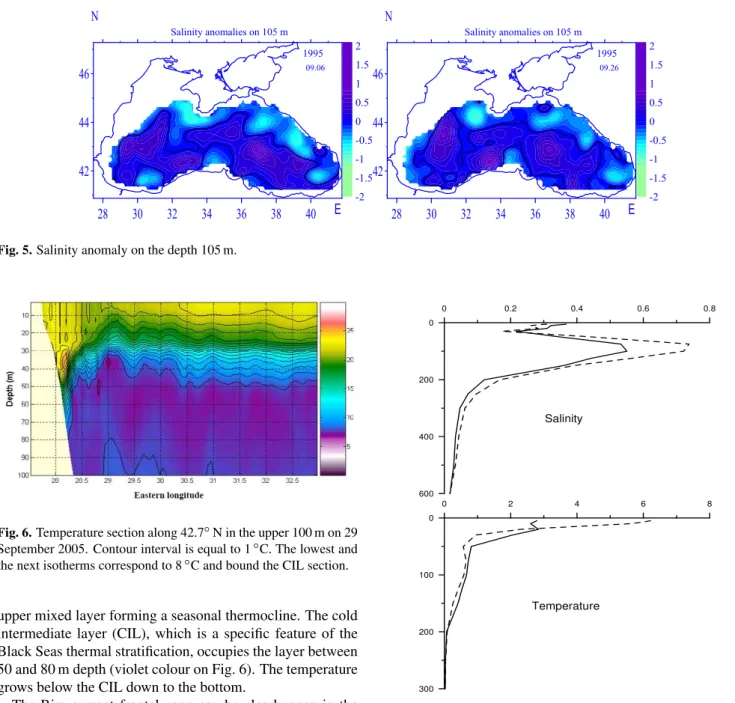
Figure 5 presents distribution of salinity anomalies at 105 m during September 1995. Light colors correspond to the salinity lower than basin-average value, and vise-versa for dark colors. Eddies of different signs are presented in deep waters according to Fig. 5. Low salinity water is prefer-entially observed in the coastal anticyclonic eddies, whereas more salty water is observed in cyclonic gyres of the interior basin. As documentred previously (Korotaev et al., 2001, 2003), the Rim current is relatively weak in the summer and fall seasons and the basin acquires more turbulent flow struc-ture of mesoscale eddies as also supported by Fig. 5.
The vertical section of water temperature along 42.7◦N is presented on Fig. 6. It illustrates a typical vertical structure of the temperature in the Black Sea. The mixed layer occupies the upper 25 m. The water temperature decreases below the
28 30 32 34 36 38 40 E 42
44 46 N
-2 -1.5 -1 -0.5 0 0.5 1 1.5 2 1995
09.06
Salinity anomalies on 105 m
28 30 32 34 36 38 40 E
42 44 46 N
-2 -1.5 -1 -0.5 0 0.5 1 1.5 2 1995
09.26
Salinity anomalies on 105 m
Fig. 5.Salinity anomaly on the depth 105 m.
Fig. 6.Temperature section along 42.7◦N in the upper 100 m on 29 September 2005. Contour interval is equal to 1◦C. The lowest and the next isotherms correspond to 8◦C and bound the CIL section.
upper mixed layer forming a seasonal thermocline. The cold intermediate layer (CIL), which is a specific feature of the Black Seas thermal stratification, occupies the layer between 50 and 80 m depth (violet colour on Fig. 6). The temperature grows below the CIL down to the bottom.
The Rim current frontal zone can be clearly seen in the left part of the section. The deepening of the thermocline as well as the Rim current jet is attached to the bottom slope. General features of the basin dynamics and stratification are well presented by model results.
3.2 Quantitative model calibration
Quantitative calibration of the simulated fields is an essential part of the Black Sea forecasting system development. This calibration is carried out with use of regular space remote sensing measurements, in situ data of hydrographic surveys, surface drifting buoys and deep profiling floats.
0 0.2 0.4 0.6 0.8
600 400 200 0
0 2 4 6 8
300 200 100 0
Salinity
Temperature
Fig. 7. Standard deviation of the differences between simulated and observed fields as a function of depth (solid lines), and the nat-ural variability (root mean square deviation from mean value) of the same fields (dash lines) (according to Dorofeyev and Korotaev, 2004a).
3.2.1 Hydrographic surveys and profiling floats
Initial tuning of the basin-scale circulation model was made against the data of four large-scale hydrographic ComsBlack surveys which were fulfilled in 1992–1995 years (Kortaev et al., 2001). The model was run with assimilation of the sea surface height (SSH). ComsBlack hydrography was used to estimate quantitatively the accuracy of 3-D temperature
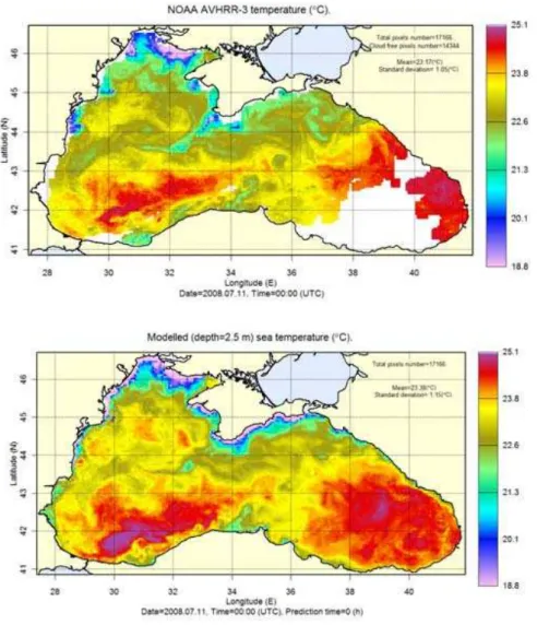
Fig. 8. SST maps on 11 July 2008 retrieved from AVHRR data (upper panel), simulated by the model (central panel) and their difference (lower panel) .
and salinity field simulations. Standard deviations of sim-ulated fields against the observed ones were calcsim-ulated on each depth level (Dorofeyev and Korotaev, 2004a). These functions are presented on Fig. 7. The standard deviation of the model analysis is compared with the natural variability of the temperature and salinity fields, i.e. with the standard deviation of the climatic data against observations.
Figure 7 shows, that the altimetry assimilation brings the most significant improvement in salinity field. It is natu-ral, because density stratification in the Black Sea depends mainly on salinity. Assimilation of altimetry allows describ-ing about 25 % of the salinity natural variability within the halocline where the difference between simulated and mea-sured fields is the most significant. In the regions of high vertical gradients even small error in the isohaline depth pro-duces large error. However simulated salinity maps agree well with observations, as it was shown earlier by (Dorofeyev and Korotaev, 2004a).
Standard deviation of temperature is the largest near the surface (here the error is greater than in the case of compari-son with buoy data). It means that the thermodynamics of the top sea layer in the model is too simplified. An explicit de-scription of the mixed layer dynamics is necessary to include for better reproduction of surface temperature by the model. Additional extremes of the temperature standard deviation are observed near the thermocline and within CIL. Increase of the error near the thermocline has the same reason, as in the case of salinity.
The correlation coefficients of simulated and observed fields of temperature and salinity are large enough. The high-est correlation for both fields occurs within the pycnocline with approximately 0.65 for salinity and 0.45 for tempera-ture.
The comparison of the model output with ComsBlack hy-drography has shown reasonable consistency of the simula-tions against observasimula-tions in deep layers of the basin and fur-ther points to the importance of SST assimilation.
3.2.2 SST calibration
Calibration of SST was one of the major issues of the ECOOP project as the space SST observations were avail-able in all basins where coastal forecasting activity was car-ried out. Development of common SST validation standards, which provide a basis for model confidence diagnosis, def-inition of a quality controlled validation database structure from distributed data centres and common protocol to cal-culate standard validation criteria was realized at the design of online model validation system to provide NRT model confidence. An experience of MERSEA, MFSTEP, ODON projects and other ongoing operational forecasting activity was taken into account for the selection of important charac-teristics and proper protocols.
On-line validation of SST analysis and three days forecast was carried out by the coastal forecasting systems and
dis-played on the ECOOP site. However SST maps produced by the basin-scale systems which provided boundary conditions for the coastal prediction, particularly the Black Sea basin-scale nowcasting/forecasting system, were calibrated off-line to achieve reasonable accuracy.
Data of IR scanner AVHRR are available in the Black Sea region through the direct reception on HRPT receiving sta-tions in Marine Hydrophysical Institute (MHI) in Sevastopol, Ukraine. Up to four IR images of the Black Sea surface are available daily. MHI processes this data regularly in the real time retrieving and mapping the Black Sea surface temper-ature. Standard NOAA algorithm is used for the retrieving of SST but the threshold for the filtration of cloudiness is ad-justed to the Black Sea conditions. Ground truth validation of IR SST against surface drifting buoys data shows its rms ac-curacy around 0.5–0.7◦(Ratner and Bayankina, 2004). SST maps retrieved from NOAA satellite observations are used to calibrate basin-scale circulation model.
Figure 8 presents typical example of SST maps retrieved from AVHRR data, analysis simulated by the model and their difference. The bias of two maps is equal 0.21◦C, standard deviation is equal 0.67◦C and correlation coefficient is equal
0.82. Statistics was simulated by averaging over the cloud free are of the Black Sea basin. At the same time the lower panel on the Fig. 8 shows that the difference between mea-sured and simulated SST in the most part of the basin area is in the range±0.5◦C. More significant difference observes
in the vicinity of frontal zones where model provides higher temperature.
Temporal evolution of the statistics is shown on Fig. 9. Mainly the statistics is similar to that presented on Fig. 8. However, sharp changes of the bias are observed on Fig. 9. Probably they are related with inconsistency of the space SST, as the model provides smooth evolution of simulated fields.
The daily averaged simulations of SST by the basin-scale model were compared also with similar data of surface drifters. It is shown (Ratner and Bayankina, 2004) that the standard deviation is in the range 0.5–0.7◦C (i.e. it is in the same range as the accuracy of SST retrieving from AVHRR data). Accuracy of SST forecast is reduced with the time of prediction. Typically bias lies in the range±0.4◦C on the
three day forecast. Standard deviation increases up to 0.9◦C for one day forecast, up to 1.1◦C for two days forecast and
up to 1.2◦C for three days forecast. Correlation coefficient
decreases approximately linearly with the prediction time up to reducing on 10 % to the third day.
3.2.3 Drifters with thermistor chain
Drifters with thermistor chain were elaborated under the sup-port of Science and Technical Center in Ukraine (project N 2241) to be able calibrate upper layer thermodynamics of the Black Sea circulation model. Drifting buoys with thermis-tor chain provide direct measurements temperature profiles
Fig. 9.Bias (blue line), standard deviation (red line) and correlation coefficient between SST retrieved from AVHRR data and simulated by the model as function of time.
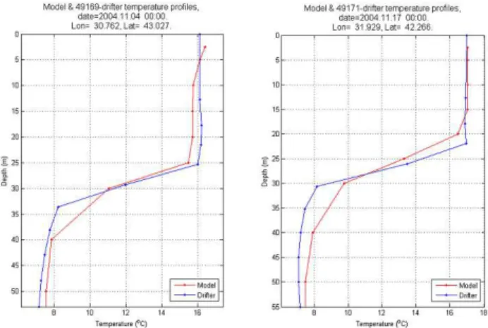
Fig. 10.Comparison of the simulated (blue line) and measured (red line) temperature profiles in the upper 70 m during the shoaling of the mixed layer.
Fig. 11.Comparison of the simulated (blue line) and measured (red line) temperature profiles in the upper 70 m during the deepening of the mixed layer.
0 2 4 6 8
200 160 120 80 40 0
0 0.2 0.4 0.6 0.8
300 200 100 0
RMST RMSS
depth depth
Figure 12 Standard deviation of the differences between simulated and measured fields as
Fig. 12. Standard deviation of the differences between simulated and measured fields as a function of depth (solid lines), and the natural variability of the same fields (dash lines).
in the upper 70 m layer of the Black Sea. Both shoaling and deepening of the seasonal thermocline were covered by ob-servations. Quality of the products of the upper layer thermo-dynamics is improved by comparing the simulated temper-ature profiles in the upper 70 m layer with direct measure-ments by the surface drifting buoys with thermistor chain. Careful tuning of the Phylander-Pakanovsky approximation to the Black Sea conditions was done by Demyshev (Demy-shev et al., 2009). Improved version of the circulation model provides reasonable description of both shoaling and deep-ening of the mixed layer (Figs. 10 and 11).
Typically the standard deviation has a maximum on the seasonal thermocline depth. Such maximum has the follow-ing explanation. There is a strong temperature gradient in the seasonal thermocline and even small inconsistency of its positioning by the model is resulted in rather significant de-viation of temperature.
3.2.4 Profiling floats
Temperature and salinity profiles are also compared with data provided by profiling floats. Figure 12 demonstrates the stan-dard deviations for temperature and salinity fields, which are
Fig. 13. Trajectories of surface drifting buoys overlapped on the simulated circulation. January 2002.
similar to those obtained by using earlier by the ComsBlack surveys (Dorofeyev and Korotaev, 2004b). The most sig-nificant deviation of simulated and measured temperature is observed in the thermocline layer (10–30 m). Temperature minimum in the cold intermediate layer on in-situ profile is more significant than on temperature profile, simulated by the model. The difference between simulated and observed temperature decrease significantly with depth.
The simulated salinity profiles differ most significantly from mesurements in the layers between 0–30 and 150– 300 m, i.e. in seasonal and permanent pycnocline where it may deviate up to 0.2 ppt. The difference between simula-tions and observasimula-tions decreases significantly below the per-manent pycnocline does not exceeding 0.05 ppt.
-80 -40 0 40 80
-80 -40 0 40 80
-80 -40 0 40 80
-80 -40 0 40 80
-60 -40 -20 0 20 40 60
-60 -40 -20 0 20 40 60
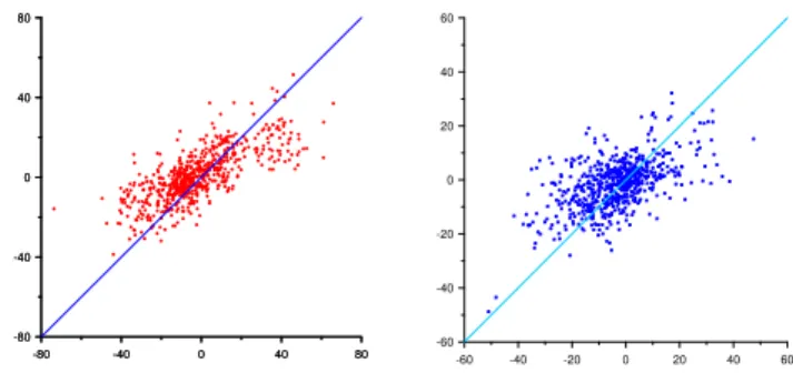
Fig. 14. Scatter plot of the simulated (vertical axe) and observed (horizontal axe) surface currents. Left and right plots correspond to zonal and meridional components of the current velocity respec-tively.
3.2.5 Surface velocity
Comparison of several drifting buoys trajectories with the simulated surface currents in January 2002 is presented in Fig. 13. Trajectories are computed from the buoy coordi-nates during three days and the simulated currents at mid-days in the figure. For example, the trajectories of the buoy numbers 7 and 14 were under the influence of Rim Current. Buoy number 14 has been captured by the current for almost a month starting from 15–16 January 2002. We note its cir-cular motion near the cape Sinop as inferred from its trajec-tories during 23 and 31 January. Buoy number 7 also has been captured by the stream of Rim Current on 23 January. It moved along the offshore side of the jet and has practically left the current on February 2002 and picked up again as they move eastward along the coast of Turkey. The buoy number 17 was located in the open part of the sea during the same period and was transported on the east by mesoscale jets pe-riodically produced as clearly seen on 31 January in Fig. 13. The trajectory of the buoy number 8 in Fig. 13 illustrates an accuracy of coastal currents simulations. The drift of buoy number 8 during 15–31 January well corresponds to the model simulated narrow coastal jet in the northeast direc-tion in the vicinity of cape Kaliakra of the Bulgarian coast. A small branch of the jet has transported the buoy number 8 towards the shore on 31 January where it remained up to the mid of February 2004. More examples of buoys trajec-tories are presented in (Korotaev et al., 2004). The evolution of current velocity along the trajectory of drifting buoy also demonstrates good reproduction of the low-frequency flow variability by the model (Korotaev et al., 2004).
The quantitative comparison of the daily averaged surface current velocity and simulations shown on Fig. 14 for zonal and meridional components. The relative error is in the range of 30 %, correlation coefficient is equal to 0.7. Neverthe-less, it is seen on Fig. 14 that the simulated velocity compo-nents are systematically underestimated by the model. This may be resulted from the different spatial averaging of the
22
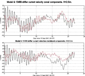
Fig. 15. Comparison of the measured (black) and simulated (red) inertial oscillations.
signal. Drifting buoys measure currents along a line whereas the model simulated velocity is averaged in the box 5×5 km.
High resolution surface current maps obtained by means of the imagery processing (Korotaev et al., 2008) show that the Rim current has fine structure in the form of narrow and in-tense submesoscale jets. However the current grid size of the model (5 km) is able to resolve mesoscale eddies but not sub-mesoscale structures. Future improvement of the Black Sea operational model should include explicit representation of submesoscale features.
Surface drifting buoys with data transmission via IRID-IUM provide a possibility to validate high-frequency vari-ability of surface currents. IRIDIUM data transmission al-lows to determine buoy coordinates often enough to de-scribe trajectory loops related to the inertial oscillations. The comparison of measured and simulated current veloc-ity oscillations at inertial frequency (Fig. 15) shows that they can strongly disturb instant surface current velocity. The model often reproduces the phase of inertial oscilla-tions whereas their amplitude usually is underestimated. Ev-idently, the accuracy of the inertial oscillation simulations depends strongly on the quality of atmospheric forcing. 3.2.6 Deep velocity
Data of profiling floats allow evaluation of the weekly av-eraged deep velocity accuracy. In general, relative accuracy of the current speed simulation by the model is highest on the depth 200 m. However weekly mean currents even on the depth 1550 m measured by profiling float and simulated by the model are in good consistency (Dorofeyev and Koro-taev, 2004b). Relative error is about 30–35 % and correlation coefficient is in the range 0.65–0.72.
4 Ecosystem model
The main part of the Black Sea ecosystem model is a bio-geochemical model. The 3D biobio-geochemical model cou-pled with the circulation model is based on the one given by Oguz et al. (2001). It has one-way coupling with circu-lation model through current velocity, temperature, salinity and turbulent diffusivity. The biogeochemical model extends to 200 m depth with 26 z-levels, compressed to the sea sur-face. It includes 15 state variables. Phytoplankton is rep-resented by two groups, typifying diatoms and flagellates. Zooplankton are also separated into two groups: microzoo-plankton (nominally<0.2 mm) and mesozooplankton (0.2– 2 mm). The carnivorous group covers the jelly-fishAurelia aurita and the ctenophoreMnemiopsis leidyi. The model food web structure identifies omnivorous dinoflagellate Noc-tiluca scintillansas an additional independent group. It is a consumer feeding of phytoplankton, bacteria, and microzoo-plankton, as well as particulated organic matter, and is con-sumed by mesozooplankton. The trophic structure includes also nonphotosynthetic free living bacteriaplankton, detritus and dissolved organic nitrogen. Nitrogen cycling is resolved into three inorganic forms: nitrate, nitrite and ammonium. Nitrogen is considered as the only limiting nutrients for phy-toplankton growth. So all these variables are presented in the model equations in units mmolN/m3. Additional com-ponents of the biogeochemical model are dissolved oxygen and hydrogen sulfide. The local temporal variations of all variables are expressed by equations of the general form
∂F
∂t +
∂(uF )
∂x +
∂(vF )
∂y +
∂((w+ws)F )
∂z (9)
=Kh∇2F +
∂ ∂z(Kv
∂F
∂z)+ ℜ(F ),
whereℜ(F )is the interaction term, which expresses a bal-ance of sources and sinks of each of biological and geo-chemical variables F; wS represents the sinking velocity
for diatoms and detrital material and is set to zero for other compartments;(u,v,w)– components of the current veloc-ity, Kh,Kv – horizontal and vertical coefficients of
turbu-lent diffusion. The last parameters are provided by physical model (the circulation model). The biogeochemical model, described here, uses the MHI or POM model output, so its space resolution is equal to the space resolution of appropri-ate circulation model.
Fluxes of all biogeochemical variables are set to zero on the sea surface, bottom in shallow part of the basin and on the lateral boundaries, except river estuaries, where nitrate fluxes are set up proportional to rivers discharges and nitrate concentrations. On the lower liquid boundary in the deep part of the basin concentrations of all parameters set to zero except ammonium and hydrogen sulfide (sulfide and ammo-nium pools).
1972 1973 100 80 60 40 20 0 0 0.2 0.4 0.6 0.8 1 1.2 1.4 1.6 1.8
J F M A M J J A S O N D
Time (months)
Depth (m)
Fig. 16.Seasonal cycle of averaged over the basin area phytoplankton derived from modelling (left panel) and chlorophyll seasonal cycle in the upper layer of the Black Sea on the basis of in-situ measurements (Vedernikov and Demidov, 1997).
100 80 60 40 20 0 0 0.5 1 1.5 2 2.5 3 3.5 4
J F M A M J J A S O N D
De pth (m ) Time (months) 100 80 60 40 20 0 0 0.2 0.4 0.6 0.8 1 1.2 1.4
J F M A J A D
Time (months)
M J S O N
De
pt
h (m
)
Fig. 17.Seasonal cycles of averaged over the basin area nitrates (left panel) and zooplankton (right panel).
5 Calibration of the ecosystem model
Analysis of the model results shows that the model repro-duces reasonably well the seasonal cycling of phytoplankton and other biochemical fields. The spring bloom of phyto-plankton computed by the model is well presented on the Fig. 14 (left). It shows also the secondary subsurface max-imum of phytoplankton on the bottom of the summer and autumn bloom. This seasonal cycle of the phytoplankton in the upper layer of the Black Sea derived from the model-ing qualitatively correspond to those obtained from measure-ments. Figure 16 exhibits on the right panel chlorophyll sea-sonal cycle in the upper layer of the Black Sea on the basis of in-situ measurements (Vedernikov and Demidov, 1997).
Figure 17 demonstrates seasonal variability of the nitrate and zooplankton concentrations in the upper layer of the Black Sea. Surface concentration of nitrate increases dur-ing the winter mixdur-ing period and reduces to small value after the spring bloom of phytoplankton. Then it remains neg-ligible until the next winter. The distribution of zooplank-ton follows closely that of phytoplankzooplank-ton with a time lag of approximately half a month. These seasonal cycles of the phytoplankton, zooplankton and nitrate in the upper layer of the Black Sea derived from the modeling qualitatively
cor-respond to those obtained from measurements (Oguz et al., 1999).
An increase of anthropogenic nutrient load together with population explosions in medusa Aurelia during the 1970s and 80s led to practically uninterrupted phytoplankton blooms in the Black Sea (Fig. 18). This figure demonstrates intra-annual variability of the phytoplankton, zooplankton biomasses and seasonal cycles ofNoctilucaand medusa Au-reliabiomasses. The left panel corresponds to the results of the modelling and the right one – to the in-situ measurements (Oguz et al., 2002). The data for phytoplankton and meso-zooplankton biomass are taken from measurements carried out at 2–4 weeks intervals during January–December 1978 at a station, off Gelendzhik along the Caucasian coast. The Noctiluca and Aurelia biomass data are taken from measure-ments on the Romanian shelf and the interior basin, respec-tively, during the late 1970s and early 1980s (after Oguz et al., 2001). The model data were chosen approximately at same places during 1978 year. The model results are in a good agreement with measurements.
An example of space distribution of the nitrate concentra-tion in the upper 20 m layer of the Black Sea is presented on the Fig. 19 (left panel). This nitrate concentration is de-rived by averaging over 4 yr the nitrate fields computed by
Fig. 18. Seasonal cycles of phytoplankton, mesozooplankton, Noctiluca and medusa Aurelia biomasses derived from modelling (left) and in-situ measurements.
Fig. 19. An example of the surface nitrate space distribution derived from the model (left) and the map built on the basis of in-situ data (fight).
1968 1972 1976 1980 1984 1988 1992 1996 2000 2004 1.2
1.6 2 2.4
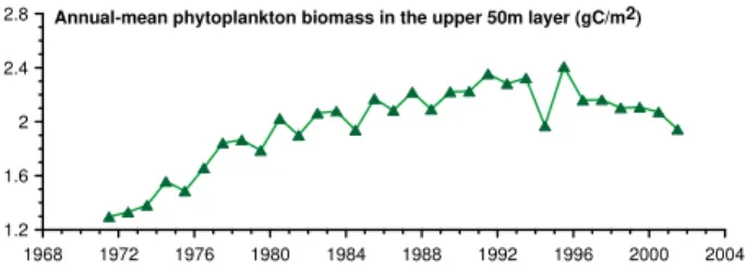
2.8 Annual-mean phytoplankton biomass in the upper 50m layer (gC/m2)
Fig. 20. Evolution of the annual-mean phytoplankton biomass in the upper 50 m layer for the deep part of the Black Sea basin.
the model. The highest values of nitrate concentration are ob-served on the northwestern shelf of the Black Sea. It is a re-sponse on nitrate supply by Danube and other rivers. High ni-trate concentration is observed also along western and south coast due to cyclonic circulation in the Black Sea. The Rim current transports part of the nitrate from northwestern shelf to the Anatolian coast. The right panel of the same Fig. 19 demonstrates mean map of the nitrate distribution in the
up-per layer obtained by using in-situ data for the tame up-period from 1957 until 2003 years (Konovalov and Eremeev, 2011). According to this map the highest concentration of the nitrate in the upper layer are typically for the coastal area on the north-western shelf near the Danube and other rivers and the lowest values can be observed in the central part of the basin. In general there is a good correspondent between these two maps.
An opportunity for qualitative calibration of the model output is given by analysis of long-term changes in the Black Sea marine ecosystem. The Black Sea marine ecosystem manifested significant changes during the last few decades of the 20th century. Healthy ecosystem which was observed in 60s, early 70s was altered drastically by eutrophication phase in 80s early 90s. These changes in the Black Sea ecosys-tem were in particular noted in the phytoplankton biomass, which increased by a few times. (See for example: Oguz et al., 2002) On the basis of the biogeochemical model de-scribed above we carried out numerical simulation of the long-term evolution of the Black Sea ecosystem for time pe-riod from 1971 until 2001 years. The input parameters for
Figure 21 Spring-mean maps of the surface phytoplankton distribution for different years.
Fig. 21.Spring-mean maps of the surface phytoplankton distribution for different years.
the biogeochemical model were the results obtained with the POM circulation model.
Figure 20 demonstrates evolution of the annual-mean phy-toplankton biomass in the upper 50 m layer for the deep part of the Black Sea basin. The phytoplankton biomass increases approximately twice from value about 1.2 gC m−2 in early seventies to 2 gC m−2in mid nineties and then it decreases. These changes in the phytoplankton biomass can also be seen in evolution of the surface concentration. The phytoplankton community exhibits a major bloom during the late winter-early spring season, following the period of active nutrient accumulation in the surface waters at the end of the winter mixing season and as soon as the water column receives suf-ficient solar radiation. The intensity of the spring bloom al-tered drastically during the time period we consider. This is
illustrated on the Fig. 21 showing spring-mean maps of the surface phytoplankton concentrations. The greatest values are observed in early 90s – period of intense eutrophication in the Black Sea. This growth of the phytoplankton commu-nity until mid of 90s is due to increase of nutrient volume in the upper layer of the Black Sea.
Changes in marine biology of the Black Sea during these three decades were accompanied by modification of the verti-cal geochemiverti-cal structure. The most pronounced signature of the geochemical changes is an increase of nitrate concentra-tion in the oxic/suboxic interface zone from 2 to 3 mmol m−3 in the late 1960s to 6–9 mmol m−3during the 1980s and early 90s, and then decrease to the value of about 4 mmol m−3in late 90s – early 2000s. Figure 22 presents nitrate profiles, de-rived from modelling, for the point placed approximately in
0 1 2 3 4 5 6 7 8 17
16 15 14 13
NO3 ( )
1971
1988
2001
t
M
Fig. 22. Derived from modeling nitrate profiles (in µM) versus sigma-t (in kg m−3) for the central western gyre (left) and nitrate profiles measured by cruise vessels (Oguz and Gilbert, 2007).
the central western gyre for three different years which cor-respond early, intense and post-eutrophication phases of the Black Sea ecosystem. The values of the nitrate maximum are in good correspondence with the measurements obtained on cruise vessels
The model was also calibrated on chlorophyll-a climato-logical fields based on the MODIS data (http://oceancolor. gsfs.nasa.gov). The model was run with input parameters corresponded to 2007 year obtained with the MHI circulation model. Numerical simulations of the Black Sea ecosystem with 5 km grid step demonstrate its ability reproducing large scale spatial features and reaction on the mesoscale dynam-ics. Figure 23 demonstrates maps of the surface chlorophyll-a computed by the model (left pchlorophyll-anel) chlorophyll-and MODIS climchlorophyll-ate, which correspond to winter, spring, summer and autumn.
Satellite color scanner measurements were used to com-pare the results of the modeling with satellite data. Fig-ure 24 demonstrates temporal variability of the basin aver-aged surface chlorophyll for the deep part of the basin de-rived from modeling (blue line) and SeaWiFS data (red line) during 2007 year. Satellite data are two week composited maps of the surface chlorophyll-a concentration, prepared for the Black Sea region (http://blackseacolor.com). The most evident deviation between satellite data and the results of the modeling can be observed in the winter seasons. Green line corresponds to RMS deviation of the model data from Sea-WiFS data.
6 Architecture of the nowcasting and forecasting system
A pilot version of the Black Sea nowcasting/forecasting sys-tem (Korotaev et al., 2006) was built in the framework of FP5 ARENA project. It operated during five days in July 2005 in the manual mode. The system architecture was improved
significantly during the next years to avoid manual operation. During ECOOP project phase it operated in real time mode. It forms version V0 of the model currently used in the My Ocean Black Sea Marine Forecasting Centre.
The software controlling the system is presented by three groups. The group of input and pre-processing consists of three sub-groups: ALTIMETRY, NOAASST and METEO. The sub-group ALTIMETRY includes downloading of SLA of missions Topex/Poseidon, ERS-2, Jason-1, Envisat and GFO from the web of AVISO centre and its pre-processing according to the algorithm described in (Korotaev et al., 2001). The sub-group NOAASST is assigned to the pre-processing of IR/AVHRR data received by the HRPT station at MHI to retrieve the SST. The sub-group METEO includes downloading of meteorological analysis and forecast of the sea surface wind, heat fluxes and precipitation/evaporation from the web of NMA (Romania) and their repacking. The group MHI-casting consists of the collection of software for the numerical process control. It provides numerical simu-lation of the Black Sea circusimu-lation, data assimisimu-lation in the circulation model and simulation of the surface wave field. The group of the output includes three sub-groups ARCH, GRAF and NET for the data archiving, graphic presentation of the system products and data distribution via Internet.
The scheme of the data flow is presented on Fig. 25. The output of the system is three dimensional temperature, salin-ity and current velocsalin-ity fields. Products of the system on the sea surface were regularly presented on the web site http://dvs.net.ua/mp as images and in digital form.
Examples of the system products presented on the web are shown on Fig. 26.
Fig. 23.Maps of the surface chlorophyll-a derived from the model (left panel) and MODIS climate data, which correspond to winter, spring, summer and autumn (from top to bottom).
2007 2008 0
0.4 0.8 1.2 1.6
J F M A M J J A S O N D
Fig. 24.Temporal evolution of the basin averaged surface chlorophyll-a (mg m∗∗3) concentration for the deep part of the basin derived from modeling (blue line), SeaWiFS data (red line) and RMS deviation (green line).
Fig. 25.Data flow in the framework of the Black Sea nowcasting/forecasting system.
7 Discussion
The pilot version of the Black Sea nowcasting and forecast-ing system which was built in the framework of the FP 5 ARENA and FP6 ASCABOS projects was significantly im-proved later during the FP6 ECOOP project. The basin-scale forecasting became operational in the real-time mode from the beginning of the ECOOP project and served as mainframe system for further development of the operational
coastal forecasting systems in the Black Sea. Started from “V0 version” it was upgraded to the Black Sea GOOS sys-tem “V2”. This last version consists of a regional syssys-tem, covering the entire Black Sea area, and 3 sub-regional sys-tems covering respectively: the North Western shelf, the Bosphorus and Western shelf, and the South coast of Crimea and North East Black sea. The paper was targeted at the description of development of the basin-wide nowcasting and forecasting system. The circulation model, which is the core
Fig. 26.Examples of the Black Sea nowcasting/forecasting system products: left – surface currents, right – sea surface temperature.
of the system, was improved during the ECOOP by including a new parameterization of the vertical mixing processes. The models have been subject to the qualitative and quantitative tests, which are the essential part of the system. Archive cli-matic, hydrographical surveys data and measurements from the drifter and profiling floats were used for the models cali-brations.
The model reproduces reasonably well upper layer ther-modynamics and vertical stratification of temperature and salinity fields, particularly upper mixed layer, cold inter-mediate layer and permanent pycnocline. Simulated cur-rent velocity displays the Rim Curcur-rent and its seasonal and mesoscale variability. Including quasi-permanent anticy-clonic eddies onshore from the stream jet. At the same time there is a broad field of work to improve the model to achieve better quantitative correspondence of the simulated fields with observations. One of possible future improvement of the qualitative skill of the model is connected with further perfection of the upper layer thermodynamics. Our experi-ence shows that current version of the model describes well relatively slow evolution of the upper layer of the sea on sea-sonal scales however less efficient when sharp atmospheric fronts crossing the basin. We assume that more efficient pa-rameterization of the mixed layer turbulence is requested in such conditions.
The accuracy of the upper layer simulations depends also on the quality of atmospheric forcing provided by meteoro-logical model. Simulations presented in the paper are based on the ALADIN family model runs with 24 km resolution. Increase of the spatial resolution of the regional atmospheric forecast and careful analysis of available atmospheric forcing for the Black Sea should permit to improve the simulation of the basin thermodynamics.
It was mentioned in the paper that the model demonstrates a slow trend in the permanent pycnocline. More careful tun-ing of vertical and lateral diffusion should help to reduce that trend. Probably better space resolution of the model allow-ing explicit resolution of submesoscales permits not only to simulate more realistic currents but also reduce temperature
and salinity trends in the permanent pycnocline.
More or less realistic simulations of the Black Sea dynam-ics are achieved due to assimilation of altimetry, space SST and climatic temperature and salinity profiles. Simple assim-ilation scheme based on the optimal interpolation is applied. Further improvement of the system efficiency demands ap-plication of more sophisticated data assimilation approaches. Optimal interpolation approach raises too high the weight of the assimilated data and generates artificial variability of ver-tical velocity according to our experience. Simulation of the error statistics as it is requested by the Kalman filter tech-nique even in simplified manner reduces mentioned above problems. Therefore transition to more sophisticated data assimilation algorithm is crucial for the improvement of the system efficiency. It is important also to assimilate available profiling float data to keep close to the reality the permanent pycnocline position and gradients as it was explained earlier. In addition the Black Sea forecasting system was added with the biogeochemical model. Together with the circula-tion model it allows describing evolucircula-tion of the Black Sea ecosystem. Calibration tests showed reasonable qualitative consistency of simulated biogeochemical parameters to the general concept of the Black Sea ecosystem annual and in-terannual evolution. Obtained results are encouraging but future improvement of the model should be done in a few directions. More careful qualitative calibration of the model should be done when multidisciplinary observations will be available in the basin. Improved model should include addi-tional compartments such as jellyfishes, important chemical elements. Implementation of the real-time space sea colour data assimilation is also important issue of the future system development.
The system architecture was improved significantly to avoid manual operation and during ECOOP project phase it operated in real time mode. The operational system estab-lished during ECOOP is the V0 version of the basin-wide nowcating and forecasting system in the frame of the FP7 My Ocean project.
Acknowledgements. The research leading to the results has re-ceived funding from the Eu ropean Community’s Sixth Framework Programme under the grant agreement No 036355 (European COastal-shelf sea Operational observing and forecasting system).
Edited by: S. Cailleau
References
Agoshkov, V. I., Ipatova, V. M., Zalesny, V. B., Parmuzin, E. I., and Shutyaev V. P.: Problems of variational assimilation of observa-tional data into Ocean general circulation models and methods for their solution, Izvestiya, Atmos. Ocean. Phys., 46, 677–712, 2010.
Arakawa, A.: Computational design for long-term numerical inte-gration of the equations of fluid motion: Two-dimensional in-compressible flow. Part I, J. Comput. Phys., 1, 119–43, 1966. Blatov, A. S., Bulgakov, N. P., Ivanov, A. N., Kosarev, A. N., and
Tujilkin, V.: Variability of the hydrodynamical fields in the Black Sea, 240 pp., Gidrometeoizdat, St. Petersburg, 1984 (in Russion). Demyshev, S. G. and Korotaev, G. K.: Numerical energy-balanced model of baroclinic currents in the ocean with bottom topography on the C-grid, in: Numerical models and results of intercalibra-tion simulaintercalibra-tions in the Atlantic ocean, Moscow, 163–231, 1992 (in Russian).
Demyshev, S. G., Dovgaya, S. V., and Markova, N. V.: Numer-ical simulations of hydrophysNumer-ical fields of the Black Sea from January to September 2006, Ecological Security of Coastal and Shelf Zone and Complex use of Shelf Resources, 19, 355–369, 2009 (in Russian).
Demyshev, S., Knysh, V., Korotaev, G., Kubryakov, A., and Mizyuk, A.: The MyOcean Black Sea from a scientific point of view, Mercator Ocean Newsletter, 39, October, 16–24, available at: http://www.mercator-ocean.fr/documents/lettre/lettre 39 en. pdf, 2010.
Dorofeyev, V. L., Demyshev, S. G., and Korotaev, G. K.: Eddy-resolving model of the Black Sea circulation, Ecological Security of Coastal and Shelf Zone and Complex use of Shelf Resources, 71–82, 2001 (in Russian).
Dorofeyev, V. L. and Korotaev, G. K.: Assimilation of the satel-lite altimetry data in the eddy-resolving model of the Black Sea circulation, Marine Hydrophys. J., 1, 52–68, 2004a (in Russian). Dorofeyev, V. L. and Korotaev, G. K.: Validation of the results of modeling the Black Sea circulation based on the data of floating buoys, Ecological Security of Coastal and Shelf Zone and Com-plex use of Shelf Resources, 11, 63–74, 2004b (in Russian). Friedrich, H. J. and St`anev, E. V.: Parameterization of vertical
dif-fusionin numerical model of the Black Sea, Small sea turbulence and mixing in the ocean, Elsevier Oceanography Series, 46, 151– 167, 1988.
Ghill, M. and Malanotte-Rizzoli, P.: Data assimilation in meteorol-ogy and oceanography, Adv. Geophys., B. Saltzmann, ed., Aca-demic Press, 33, 141–266, 1991.
Knysh, V. V., Saenko, O. A., and Sarkisyan, A. S.: Method of assim-ilation of altimeter data and its test in the tropical North Atlantic, Rus. J. Numer. Anal. Math. Modelling, 11, 5, 333–409, 1996. Knysh, V. V., Kubryakov, A. I., Inyushina, N. V., and Korotaev, G.
K.: Reconstruction of the climatic seasonal Black Sea circula-tion by means of sigma-coordinate model and assimilacircula-tion of the
temperature and salinity data, Ecological safety of coastal and shelf zone and complex use of their resources, Sevastopol, 12, 243–265, 2005 (in Russian).
Konovalov, S. K. and Eremeev, V. N.: Monitoring of the Black Sea Biogeochemical Properties: Major Fiatures and Changes, in press, 2011.
Korotaev, G. K., Saenko, O. A., and Koblinsky, C. J.: Satellite al-timetry observations of the Black Sea level, J. Geoph. Res., 106, C1, 917–933, 2001.
Korotaev, G. K., Oguz, T., Nikiforov, A. A., and Koblinsky, C. J.: Seasonal, interannual and mesoscale variability of the Black Sea upper layer circulation derived from altimeter data, J. Geoph. Res., 108, 3122, doi:10.1029/2002JC001508, 2003.
Korotaev, G. K., Dorofeyev, V. L., and Smirnova, T. Yu.: Accu-racy of the diagnosis of surface currents in the system of the Black Sea satellite monitoring, Ecological Security of Coastal and Shelf Zone and Complex use of Shelf Resources, 11, 75–92, 2004 (in Russian).
Korotaev, G. K., Cordoneanu, E., Dorofeyev, V. L, Fomin, V., Grig-oriev, A. V., Kordzadze, A., Kubryakov, A. I., and Oguz, T.: Near-operational Black Sea nowcasting/forecasting system, in: European Operational Oceanography: Present and Future, 4th EuroGOOS Conference, 6–9 June 2005, Brest, France, 2006. Korotaev, G. K., Huot, E., Le Dimet, F.-X., Herlin, I., Stanichny,
S. V., Solovyev, D. M., and Wu, L.: Retrieving ocean surface current by 4-D variational assimilation of sea surface temperature images, Remote Sens. Environ., 112, 4, 1464–1475, 2008. Mellor, G. L., and Yamada, T.: Development of a turbulence
clo-sure model for geophysical fluid problems, Rev. Geophys. Space Phys., 20, 851–875, 1982.
Obukhov, A. M.: Turbulence in temperature heterogeneous atmo-sphere, Proceedings of Institution of Theoretical Physics SU Academy of Science, 24, 3–42, 1946.
Oguz, T., Latun, V. S., Latif, M. A., Vladimirov, V. V., Sur, H. I., Makarov, A. A., Ozsoy, E., Kotovshchikov, B. B., Eremeev, V., and Unluata, U.: Circulation in the surface and intermediate layers of the Black Sea, Deep Sea Res. Pt. I, 40, 1597–1612, 1993.
Oguz, T., Ducklow, H. W., Malanotte-Rizzoli, P., Murray, J. W., Shushkina, E. A., Vedernikov, V. I., and Unluata, U.: A physical-biochemical model of plankton productivity and nitrogen cycling in the Black Sea, Deep-Sea Res., Pt. I, 46, 4, 597–636, 1999. Oguz, T., Ducklow, H. W., and Malanotte-Rizzoli, P.: Modeling
distinct vertical biochemical structure of the Black Sea: Dynam-ical coupling of the oxic, suboxic, and anoxic layers, Global Biochem. Cy., 14, 4, 1331–1352, 2000.
Oguz, T., Ducklow, H. W., Purcell, J. E., and Malanotte-Rizzoli, P.: Modeling the response of top-down control exerted by gelatinous carnivores on the Black Sea pelagic food web, J. Geophys. Res, 106, C3, 4543–4564, 2001.
Oguz, T., Malanotte-Rizzoli, P., Ducklow, H. W., and Murray J. W.: Interdisciplinary Studies Integrating the Black Sea Biogeo-chemistry and Circulation Dynamics, Oceanography, 15(3), 4– 11, 2002.
Oguz, T. and Gilbert, D.: Abrupt transitions of the top-down con-trolled Black Sea pelagic ecosystem during 1960-2000: evidence for regime shifts under strong fishery exploitation and nutrient enrichment modulated by climate-induced variations. Deep-Sea Res Pt. I, 54, 220-242, 2007.
Pacanovsky, R. C. and Philander, G.: Parameterization of verti-cal mixing in numeriverti-cal models of the tropiverti-cal ocean, J. Phys. Oceanogr., 11, 1442–1451, 1981.
Ratner, Yu.B. and Bayankina, T. M.: Comparison of the surface temperature values obtained from the model of the Black Sea dynamics and the data of SVP-drifters in March-August 2003, Ecological Security of Coastal and Shelf Zone and Complex use of Shelf Resources, 11, 51–62, 2004 (in Russian).
Sur, H. I., Ozsoy, E., and Unluata, U.: Boundary current instabili-ties, upwelling, shelf mixing and eutrophication processes in the Black Sea, Progr. Oceanogr., 33, 249–302, 1994.
Vedernikov, V. I. and Demidov, A. B.: Vertical distributions of pri-mary production and chlorophyll during different seasons in deep part of the Black Sea, Oceanology, Engl. Transl., 37, 376–384, 1997.
Zalesny, V., Tamsalu, R., and Mannik, A.: Multidisciplinary numer-ical model of a coastal water ecosystem, Russ. J. Numer. Anal. Math. Modelling, 23, 2, 207–222, 2008.
Zalesny, V. B. and Tamsalu, R.: High-resolution modeling of a marine ecosystem using the FRESCO hydroecological model. Izvestiya, Atmos. Ocean. Phys., 45, 108–122, 2009.