Study of Stability of Rotational Motion of Spacecraft with Canonical Variables

(1)

Volume 2012, Article ID 137672,19pages doi:10.1155/2012/137672

Research Article

Study of Stability of Rotational Motion of

Spacecraft with Canonical Variables

William Reis Silva,

1

_{Maria Cec´ılia F. P. S. Zanardi,}

1

Regina Elaine Santos Cabette,

2, 3

and Jorge Kennety Silva Formiga

3, 4

1_{Group of Orbital Dynamics and Planetology, S˜ao Paulo State University (UNESP),}

Guaratinguet´a 12516-410, SP, Brazil

2_{Department of Mathematics, S˜ao Paulo Salesian University (UNISAL), Lorena 12600-100,}

SP, Brazil

3_{Space Mechanic and Control Division, National Institute for Space Research (INPE),}

S˜ao Jos´e dos Campos 12227-010, SP, Brazil

4_{Department of Aircraft Maintenance and Aeronautical Manufacturing, Faculty of}

Technology (FATEC), S˜ao Jos´e dos Campos 12247-004, SP, Brazil

Correspondence should be addressed to William Reis Silva,reis.william@gmail.com

Received 16 July 2011; Revised 10 October 2011; Accepted 23 October 2011

Academic Editor: Tadashi Yokoyama

Copyrightq_{2012 William Reis Silva et al. This is an open access article distributed under the} Creative Commons Attribution License, which permits unrestricted use, distribution, and reproduction in any medium, provided the original work is properly cited.

This work aims to analyze the stability of the rotational motion of artificial satellites in circular orbit with the influence of gravity gradient torque, using the Andoyer variables. The used method in this paper to analyze stability is the Kovalev-Savchenko theorem. This method requires the reduction of the Hamiltonian in its normal form up to fourth order by means of canonical transformations around equilibrium points. The coeﬃcients of the normal Hamiltonian are indispensable in the study of nonlinear stability of its equilibrium points according to the three established conditions in the theorem. Some physical and orbital data of real satellites were used in the numerical simulations. In comparison with previous work, the results show a greater number of equilibrium points and an optimization in the algorithm to determine the normal form and stability analysis. The results of this paper can directly contribute in maintaining the attitude of artificial satellites.

1. Introduction

Stability analysis of the rotational motion of a satellite taking into account the influence of external torques is very important in maintaining the attitude to ensure the success of a space mission.

Recently, some studies on the subject have been developed, and they motivated the

development of this paper. In 1,2 is presented a study on the stability of the rotational

(2)

gradient torque, using canonical formulations and the Andoyer canonical variables. These

studies use the procedure presented in3to determine a normal form of the Hamiltonian up

to 4th order.

In4is developed a numerical-analytical method for normalization of Hamiltonian

systems with 2 and 3 degrees of freedom. The normal form is obtained using the Lie-Hori

method5. The stability analysis of the system is made by the Kovalev-Savchenko theorem

6. The most important role of this work is the results obtained analytically for the generating function of 3rd order, necessary for determining the coeﬃcients of the normal Hamiltonian of 4th order.

Thus, the objective of this work is to optimize the stability analysis developed in

2 to determine the equilibrium points, the normal form for dynamical systems with two

degrees of freedom, and the applications of the Kovalev-Savchenko theorem 6. It will be

done by applying the expressions obtained in4for the coeﬃcients of the normal 4th-order

Hamiltonian.

In this paper equilibrium points and/or regions of stability are established when parcels associated with gravity gradient torque acting on the satellite are included in the equations of rotational motion.

The Andoyer variables are used to describe the rotational motion of the satellite in order to facilitate the application of methods of stability of Hamiltonian systems.

The Andoyer canonical variables 7 are represented by generalized momentsL1, L2, L3

and by generalized coordinates ℓ1, ℓ2, ℓ3 that are outlined in Figure 1. The angular

variablesℓ1, ℓ2, ℓ3 are angles related to the satellite system Oxyz with axes parallel to the

spacecraft’s principal axes of inertiaand equatorial system OXYZwith axes parallel to the

axis of the Earth’s equatorial system. Variables metricsL1,L2,L3are defined as follows:L2

is the magnitude of the angular momentum of rotationL2, L1 is the projection ofL2 on the

z-axis of principal axis system of inertiaL1 L2cosJ2, whereJ2 is the angle between the

z-satellite axis andL2, andL3 is the projection ofL2on the Z-equatorial axisL3 L2cosI2,

whereI2is the angle between Z-equatorial axis andL2.

The nonlinear stability of equilibrium points of the rotational motion is analyzed here

by the Kovalev-Savchenko theorem6, which requires the normalized Hamiltonian up to

terms of fourth order around the equilibrium points.

The equilibrium points are found from the equations of motion. With the application of the Kovalev-Savchenko theorem, it is possible to verify if they remain stable under the influence of terms of higher order of the normal Hamiltonian.

In this paper numerical simulations were made for two hypothetical groups of artificial satellites, considering them in a circular orbit and with symmetric shape in relation to their physical and geometric characteristics. The satellites are classified as medium and small sized; they have orbital data and physical characteristics similar to real satellites.

2. Equations of Motion

The Andoyer variables, defined above, are used to characterize the rotational motion of a

satellite around its center of mass7, and the Delaunay variables describe the translational

motion of the center of mass of the satellite around the Earth8.

The Delaunay variables L, G, H, l, g, h are defined as 8 L M√µa, G

(3)

Plane perpendicular

Equatorial plane

X

Z

x

z

y

principal axis of inertia

to the angular momentum vector Plane perpendicular to the

Y

L1 L2

L3

J2

I2

I2 l1

l2

l3

ym zm

xm

O

Figure 1:The Andoyer canonical variables.

of the ascending node,Mis the mass of the satellite,µis the Earth gravitational parameter,I

is the inclination of the orbit,ais the semimajor axis, andeis the orbital eccentricity.

Here it is assumed that the satellites are in a circular orbit, which diﬀers from the

study presented in2which considers satellites in eccentric orbits. This consideration was

adopted to simplify the Hamiltonian of the problem, which is extensive1, and to facilitate

the stability analysis of the equilibrium points.

Thus, assuming that the satellites have well-defined circular orbit, the main focus of the work is only aimed at stability analysis of the rotational movement of the satellites in study.

In this case the Hamiltonian of the problem is expressed in terms of the Andoyer and

Delaunay variables9as follows:

F

L1, L2, L3, ℓ2, ℓ3, L, G, H, l, g, hFoL, L1, L2 F1L1, L2, L3, ℓ2, ℓ3, L, G, H, l, g, h, 2.1

whereFois the unperturbed Hamiltonian andF1 is the term of the Hamiltonian associated

with the disturbance due to the gravity gradient torque, both are described respectively by 10

Fo− µ2_M3

2L2

1 2

₁

C−

1

2A−

1

2B

L12

1 2

₁

A

1

B

L22

₁

4

₁

B−

1

A

L22−L12

cos 2ℓ1,

F1 µ4_M6

L6 ₂_C

−A−B

2 H1ℓm, Ln

A−B

4 H2ℓm, Ln ,

(4)

wherem2,3 andn1,2,3;A, B, andCare the principal moments of inertia of the satellite

onx-axis,y-axis, andz-axis, respectively;H1andH2are functions of the variablesℓm, Ln,

whereℓ2 andℓ3 appear in the arguments of cosines. The complete analytical expression is

presented in1for eccentric orbits. In this paperF1will be simplified considering the satellite

in a circular orbit; its complete analytical expression is given in the Appendix.

Thus, the equations of motion associated with the Hamiltonian2.1are given by

dℓi

dt

∂F ∂Li

, dLi

dt −

∂F ∂ℓi

i1,2,3. 2.3

These equations are used to find the possible equilibrium points of the rotational movement.

In this study, it is also considered that the satellite has two of its principal moments

of inertia equal, B A. With this relationship, the variable ℓ1 will not be present in the

Hamiltonian, reducing the dynamic system to two degrees of freedom, a necessary condition for applying the stability theorem chosen for analysis of equilibrium points.

3. Determining the Normal Form of the Hamiltonian of

the Rotational Motion

3.1. Normal Form of the Hamiltonian of 2nd Order and

Linear Stability Analysis

Because the variable ℓ1 is a cyclic coordinate, the Hamiltonian 2.1 is written as

FL2, L3, ℓ2, ℓ3and the equations of motion2.3can be written in vector form as1

˙

wJFw, 3.1

wherewis the state vector and Fwis the matrix of partial derivatives with respect to their

respective variables given by

w

⎛

⎜ ⎜ ⎝

ℓ2 L2 ℓ3 L3

⎞

⎟ ⎟

⎠, Fw

⎛

⎜ ⎜ ⎜ ⎜ ⎜ ⎜ ⎜ ⎜ ⎜ ⎜ ⎜ ⎜ ⎝

∂F ∂ℓ2 ∂F ∂L2

∂F ∂ℓ3 ∂F ∂L3

⎞

⎟ ⎟ ⎟ ⎟ ⎟ ⎟ ⎟ ⎟ ⎟ ⎟ ⎟ ⎟ ⎠

3.2

andJa symplectic matrix given by

J

⎛

⎜ ⎜ ⎝

0 1 0 0

−1 0 0 0

0 0 0 1

0 0 −1 0

⎞

⎟ ⎟

(5)

Now, it is necessary to linearize the system around the equilibrium point. However,

it is convenient to make a translation of the coordinates in the Hamiltonian2.1so that the

origin coincides with the equilibrium point under study; it means that

L1L1e, ℓ2ℓ2e q1, L2L2e p1, ℓ3ℓ3e q2, L3L3e p2,

3.4

whereL1e, ℓ2e, L2e, ℓ3e, andL3eare the coordinates of equilibrium points.

With this translation we can expand the Hamiltonian in Taylor series around the new origin that is nothing more than expand the Hamiltonian in the neighborhoods of the

equilibrium point whenq1p1q2 p20. Then,

Fℓm, Ln ∞

k2

Fkℓm, Ln F2ℓm, Ln F3ℓm, Ln F4ℓm, Ln · · ·, 3.5

wherem2,3,n1,2,3, andFkis the Hamiltonian expanded up to terms of orderk, with

k2,3,4,. . . .

The HessianPof the problem is calculated from the Hamiltonian expanded up to 2nd

order around the equilibrium point:

P ⎛ ⎜ ⎜ ⎜ ⎜ ⎜ ⎜ ⎜ ⎜ ⎜ ⎜ ⎜ ⎜ ⎜ ⎝

∂2_F ∂q2 1

∂2_F ∂q1∂p1

∂2_F ∂q1∂q2

∂2_F ∂q1∂p2 ∂2_F

∂p1∂q1 ∂2_F ∂p2 1

∂2_F ∂p1∂q2

∂2_F ∂p1∂p2 ∂2_F

∂q2∂q1 ∂2_F ∂q2∂p1

∂2_F ∂q2 2

∂2_F ∂q2∂p2 ∂2_F

∂p2∂q1 ∂2_F ∂p2∂p1

∂2_F ∂p2∂q2

∂2_F ∂p2₂

⎞ ⎟ ⎟ ⎟ ⎟ ⎟ ⎟ ⎟ ⎟ ⎟ ⎟ ⎟ ⎟ ⎟ ⎠ . 3.6

Thus, the system of linearized equations can be written as

˙

WJPW, 3.7

whereWis the state vector in the new variables

W ⎛ ⎜ ⎜ ⎝ q1 p1 q2 p2 ⎞ ⎟ ⎟

(6)

So, to find the eigenvalues of the reduced linear system, we should diagonalize the

matrixJPpresent in3.7by means of the determinant detλI₋JP 0, whereIis an identity

matrix andλ are the eigenvalues of the matrixJP. If these eigenvalues are pure imaginary

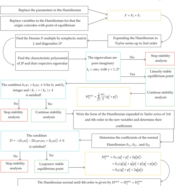
λj ±iωj, the normal form of 2nd-order Hamiltonian can be expressed as2

H₂∗

qj, pj 2

j1 ωj

2

qj2 pj2

. 3.9

3.2. Extension of the Normal Form of the Hamiltonian to Higher Orders

Extending the process of normalization of the Hamiltonian to higher ordersH3, H4, . . ., the

Hamiltonian normal in terms of variablesqiandpican be expressed by

H

qj, pj 2

j1 ωi

2

qj2 pj2

H₃∗

qj, pj H4∗

qj, pj · · · . 3.10

To obtain the Hamiltonian normalH∗

3, H4∗, . . ., it is necessary to use the method of

Lie-Hori. According to11, it is desirable that the normal Hamiltonian is written in complex

variables before using this method.

This transformation of variables is given by

qj √1

2

xj iyj, pj √1

2

ixj yj 3.11

with inverse given by

xj √1

2

qj−ipj, y_j √1

2

−iqj pj. 3.12

Thus, the normal Hamiltonian of 2nd order is given by

H₂∗

xj, yj 2

j1

iωjxjyj 3.13

and normal Hamiltonian until the 4th order in complex variables is represented by

H∗

xj, yj 2

j1

iωjxjyj H3∗

xj, yj H4∗

(7)

whereH∗

3x, yandH4∗x, ycan be expressed briefly as

H₃∗ x, y

|α| _|β_|3

h3,α,βxαyβ, _3.15

H₄∗ x, y

|α| _|β_|4

h4,α,βxαyβ. _3.16

In3.15and3.16, is always assumed itα, β >0. For3.15,|α| |β| 3 means that

the sum of the exponents of the new variables must obey the order of the HamiltonianH∗

3,

and, for3.16,|α| |β| 4 means that the sum of the exponents of the new variables must

obey the order of the Hamiltonian H∗

4. These equations are presented entirely in1,4.

Thus, we have the Hamiltonian written in complex variables. It is important to note

thatH2 is already normalized, and now we can apply the method of Lie-Hori to find the

normal form to higher ordersH₃∗, H₄∗.

3.2.1. Series Method of Lie-Hori

The normal form is obtained from the expansion of the Hamiltonian in terms of the Lie series

given by12,13

HnewH∗ {H∗, G} _2!1{{H∗, G}, G} _3!1{{{H∗, G}, G}, G} · · ·, 3.17

where Hnew _{is normal Hamiltonian obtained by canonical transformations around the}

equilibrium point,GGxi, yiis the generating function developed as a power series, where

each degree ofGnis a sum of homogeneous polynomials of degreen,H∗ H∗x, yis the

original Hamiltonian, and{H∗_{, G}_}_{is the Poisson brackets of order}_r _s₋_{2, where}_r _and_s

represent the order of the polynomialsH∗_and_G_{, respectively.}

The Poisson bracket is defined as

{H∗, G} ∂H∗

∂x ∂G ∂y −

∂H∗

∂y ∂G

∂x. 3.18

The new HamiltonianHnew _{after the new canonical transformation in the}

neighbor-hoods of identity can be expressed as2

(8)

So the new Hamiltonian, ordered by degree up to 4th order, can be expressed following

the next form11,13:

2nd order: H₂newH₂∗, 3.20

3rd order: H₃newH₃∗

H₂∗, G3

, 3.21

4th order: Hnew

4 H4∗

H₃∗, G3

1 2!

H₂∗, G3, G3 H2∗, G4. 3.22

AsHnew

2 is already given in its normal form, the next step is to calculate the generating

function which leads to the normal form up to 4th-order terms. This procedure allows to

obtain the minimum number of nonresonant monomials defined in12; thus, the generating

function Gn is chosen to eliminate the complex variables in the total Hamiltonian 3.5 in

which the monomials xj and yj have diﬀerent exponents of the desired degree, leaving

only the monomials that carry on the resonance of the intrinsic Hamiltonian systems. The

following is a procedure to obtain the normal Hamiltonian to 4th order1,4.

IIt is known that Hamiltonian systems are naturally resonant in even orders, 2nd,

4th, and so forth 10, 12, so to find the normal Hamiltonian until the 4th order, the 3rd

disturbanceH₃newmust first be removed fromHnew_{, it means}

H₃new0. 3.23

AssumingH∗

3 is briefly defined in3.15to eliminate terms of 3rd order, we consider

the generating functionG3x, yexpressed in abbreviated form as

G3 x, y

|α| _|β_|3

g3,α,βxαyβ. 3.24

Then it is necessary to find G3x, y of the third-order homological equation3.21,

where

H₂∗, G3−H3∗. 3.25

After some algebraic manipulations, we findG3x, ygiven by4

G3x, y

|α| _|β_|3

− h3,α,β β−α, Wx

α_yβ_. _3.26

Note that this equation is well defined ifβ−α, W/0, whereβ−α, Wrepresents

an inner product between β₋α β1 −α1, β2−α2, . . . , βn −αnandW λ1, λ2, . . . , λn

iω1, iω2, . . . , iωnwhich are pure imaginary eigenvalues obtained from the quadratic part of

normal Hamiltonian. The complete analytical representation forβ−α, Wwas presented in

(9)

For the resonance condition it is not accepted thatβ−α, W/0, which is always true for monomials of third-order Hamiltonian when considering only the natural resonance of the Hamiltonian.

IIThis process is repeated for the polynomial of degree 4 findingG4x, ythat will

eliminate some of monomials H₄∗ in 3.16. The remaining monomials in H₄new are called

resonant monomials3. Then3.22can be reduced as1

G4, H2∗

H₄newH₄∗

H₃∗, G3

1 2!

H₂∗, G3, G3, 3.27

G4, H2∗

H₄newF4. 3.28

Equation3.28is called homological equation of 4th order, and it can be rewritten as

G4, H2∗

F4−H4new,

G4, H2∗

R4.

3.29

Assume thatR4x, yandG4x, ywill be expressed in short form as

R4 x, y

|α| _|β_|4

r4,α,βxαyβ, _3.30

G4 x, y

|α| _|β_|4

g4,α,βxαyβ. _3.31

After some algebraic manipulations, we findG4x, ygiven by4

G4 x, y

|α| |β_|4 r4,α,β

α−β, Wx

α_yβ_, _3.32

whereα−β, W/0 represents an inner product as mentioned above.

Thus, using 3.34 in 3.29 it is possible to find Hnew

4 after some algebraic

manipulations.

This procedure can be repeated for any order that is required in order to find a normal

form of the new HamiltonianHnew_{. In this paper it is considered the 4th order of the}_Hnew_.

3.3. Normal Form of the Hamiltonian of 4th Order and

Nonlinear Stability Analysis

As we get the normal form of 2nd-order Hamiltonian 3.9, we can apply the method

described previously to find the Hamiltonian normal until the 4th order using the

Hamiltonian in complex variables3.14represented by1,4

H∗

xj, yjiω1x1y1 iω2x2y2 H3∗

x1, y1, x2, y2 H4∗

(10)

whereH∗

3x1, y1, x2, y2andH4∗x1, y1, x2, y2are obtained from expressions

H3∗x1, y1, x2, y2

|α| _|β_|3

h3,α1,β1,α2,β2x1

α1_y

1β1x2α2y2β2,

H₄∗

x1, y1, x2, y2

|α| _|β_|4

h4,α1,β1,α2,β2x1

α1_y

1β1x2α2y2β2.

3.34

Using the method of Lie-Hori presented before, it is possible to determine the

generating function G3x1, y1, x2, y2 in order to satisfy the homological equation 3.25,

where G3x1, y1, x2, y2 was determined analytically in 4. This generating function is

responsible for the elimination of the 3rd-order terms of the Hamiltonian3.33.

The generating functionG3x1, y1, x2, y2 is used to find the terms of 4th order, F4,

and perform the separation described in 3.28, obtaining H4 and G4x1, y1, x2, y2. The

coeﬃcients of the normal formHnew

4 can be calculated using the terms obtained inH4and

the eigenvalues ofH2.

Thus, the normal Hamiltonian in complex variables separated by degree can be expressed as follows4:

2nd order: Hnew

2 iω1x1y1 iω2x2y2, 3.35

3 rd order: H₃new0, 3.36

4th order: H₄newδ11

x1y12 δ12

x1y1x2y2 δ22

x2y22

, 3.37

whereωjj 1,2is the imaginary part of eigenvalues associated with the matrix defined by

the product of a matrix symplectic of order 4 with the Hessian of the Hamiltonian expanded

in Taylor series up to 2nd order around the equilibrium point;δijare real coeﬃcients obtained

from the combination ofhk,α,βxαyβ k3,4.

However, the Kovalev-Savchenko theorem requires that the normal Hamiltonian is in

real variables, and with the applications of the transformation of variables3.12the normal

form Hamiltonian can been expressed as follows:

2nd order: H₂new ω1

2

q12 p12

ω₂

2

q22 p22

, 3.38

3 rd order: H₃new0, 3.39

4th order: Hnew

4 δ11

q14 p14 2q12p12

δ12

q12q22 q12p22 p12q22 p12p22

δ22

q24 p24 2q22p22

,

3.40

where δij are the coeﬃcients of the Hamiltonian normal 4th order which are expressed

(11)

4. Kovalev-Savchenko Theorem

To use the stability theorem, the normal Hamiltonian of the problem is necessary as it was discussed above.

Considering the normal HamiltonianHo_{, an analytics function of coordinates}_q

νand

generalized momentspνto a fixed pointPis expressed by

Ho

2

ν1 ωo

ν

2 Rν

2

ν,υ1 δo

ν,υ

4 RνRυ O5, 4.1

whereO5represents higher-order terms;ωoνis the imaginary part of eigenvalues associated

with the matrix defined by the product of a 4th-order matrix symplectic with the Hessian of the Hamiltonian expanded in Taylor series up to 2nd order around the equilibrium point;

δo

ν,υdepend on the eigenvaluesωoνand the coeﬃcients of the Hamiltonian expanded in Taylor

series of 3rd and 4th order around the equilibrium point and they are presented analytically

in Formiga4, and

Rmqm2 pm2 withm1,2. 4.2

The stability analysis is performed here by the Kovalev-Savchenko theorem6which

ensures that the motion is Lyapunov stable if the following conditions are satisfied.

iThe eigenvalues of the reduced linear system are pure imaginary±iωo₁and±iωo₂.

iiThe condition

k1ω₁o k2ωo₂/0 4.3

is valid for allk1andk2integers satisfying the inequality

|k1| |k2| ≤4. 4.4

iiiThe determinantDo_{must satisfy the inequality}

Do₋δo₁₁ωo₂2−2δ₁₂oωo₁ωo₂ δ₂₂oωo₁2/0, 4.5

whereδo

ν,υare the coeﬃcients of the normal 4th-order Hamiltonian.

This theorem says that a Hamiltonian reduced in its normal form up to 4th order, in

the absence of the resonance condition of the eigenvalues associated and if the condition4.5

is satisfied, it is guaranteed the existence of tori invariant in a neighborhood small enough of

(12)

Figure 2:Flowchart representative of the stability analysis of equilibrium points.

5. Computational Algorithm for the Normal Form of the Hamiltonian

of Rotational Motion and Analysis of Stability

In order to synthetize the process to analyze the stability of equilibrium points, the logical sequence of the algorithm is now presented.

5.1. Stability Analysis of Equilibrium Points

(13)

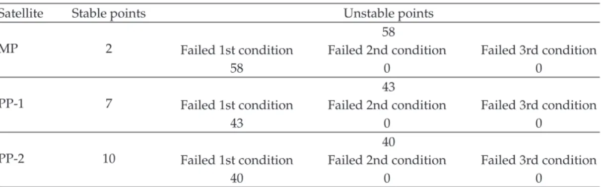
Table 1:Quantitative summary of the classification of equilibrium points.

Satellite Stable points Unstable points

MP 2

58

Failed 1st condition Failed 2nd condition Failed 3rd condition

58 0 0

PP-1 7

43

43 0 0

PP-2 10

40

40 0 0

6. Numerical Simulations

As already mentioned, we consider two types of satellites: medium sized MP, which

has similar orbital characteristics with the American satellite PEGASUS 17, and small

sizedPP, which has similar orbital characteristics of the Brazilian data collection satellite

SCD-1 and SCD-2 18. All the numerical simulations were developed using the software

MATHEMATICA.

Table 1 shows a quantitative summary of the equilibrium points found and their

stability, according to the criteria of Kovalev-Savchenko theorem6. It can be observed that,

when the first condition is not satisfied, the eigenvalues associated with the matrixJP are

real or are not pure imaginary. This equilibrium point is not linearly stable.

There were found totals of 60 equilibrium points for the MP satellite, 50 equilibrium

points to the PP-1 satellite and 50 equilibrium points for the PP-2 satellite. Tables2,3and4,

show two equilibrium points found in the simulations, one being Lyapunov stable and the other unstable, to satellites MP, PP1 and PP2, respectively.

For the Lyapunov stable equilibrium points of Tables2,3, and4respectively,Table 5

shows the values of the angles I2, J2, the rotation speed ω, and the rotation period T.

These values characterize the nonexistence of singularities in these points; it means that

the anglesI2 and J2 are not null or close to zero. ByFigure 1, when these anglesI2 and J2

are null or close to zero, the Andoyer variablesl1,l2, andl3 are indeterminate, because it is

diﬃcult to determine the intersection between the involved planes in the definitions of these variables. This analysis was performed for all equilibrium points found in the simulations.

Table 6shows the same conditions for the unstable points of Tables2,3, and4.

7. Conclusion

In this paper we presented a semianalytical stability of the rotational motion of artificial satellites, considering the influence of gravity gradient torque for symmetric satellite in a circular orbit. Applications in numerical simulations, performed with the software

MATHEMATICA, were made to two types of satellites: mediumMPand smallPP.

(14)

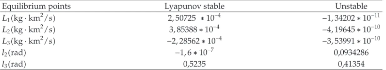
Table 2:Satellite MP:AB3,9499∗10−1kg·km2_,_C₁_,₀₃₀₇_∗₁₀−1_kg ·km2_.

Equilibrium points Lyapunov stable Unstable

L1kg·km2/s 2,50725 ∗10−4 −1,34202∗10−11

L2kg·km2/s 3,85388∗10−4 −4,19645∗10−10

L3kg·km2/s −2,28562∗10−4 −3,53991∗10−10

l2rad −1,6∗10−7 0,0934286

l3rad 0,5235 0,41354

Table 3:Satellite PP-1:AB9.20∗10−6_kg_·_km2_,_C₁₃_∗₁₀−6_kg_·_km2_.

L1kg·km2/s 2,69365∗10−7 7,13725∗10−11

L2kg·km2/s 2,07921∗10−5 2,14416∗10−10

L3kg·km2/s 1,05633∗10−5 1,07843∗10−10

l2rad 0,066560 −0,090962

l3rad 0,4 0,07

Table 4:PP-2:AB28,7∗10−4kg·km2_,_C₃₆_,₉_∗₁₀−4_kg

·km2_.

L1kg·km2/s 6,25509∗10−5 2,48081∗10−11

L2kg·km2/s 7,24797∗10−4 2,77796∗10−11

L3kg·km2/s 2,17564∗10−4 −2,54792∗10−11

l2rad 0,098581 −1,68042

l3rad 1,42527 1,05253

For the satellite MP it was gotten only two equilibrium points because this satellite

has similar characteristics to the satellite PEGASUS, which is tumbling17. For satellites

PP-1 and PP-2 were obtained many other equilibrium points, but most of them were discarded,

because they lead to the Andoyer variables, a condition of uniqueness it means that the

angles I2 and J2 are null or close to zero, and the Andoyer variables l1, l2, and l3 are

indeterminate.

It can be observed that a larger number of stable equilibrium points were determined

in comparison with the results of1,2, which show the stability analysis of the rotational

motion with the gravity gradient torque, but with the satellite in an elliptic orbit.

An optimization was done in the algorithm of determining the normal form of the

Hamiltonian and the stability analysis, using expressions obtained by4for the coeﬃcients

of the normal 4th-order Hamiltonian. The introduction of these expressions enabled a more

eﬀective stability analysis for equilibrium points in comparison with the results of1,2. It is

possible to say that the numerical simulations have become less laborious allowing analysis of data in more numbers .

(15)

Table 5:Analysis of possible singularities of the Anloyer variables for satellites MP, PP1 of and PP2.

Lyapunov stable equilibrium point ofTable 2,3and4, respectively.

Satellite I2rad J2rad ωrad/s T s Situation

MP 2,20566 0,862451 0,00373909 1680,4 Accepted PP-1 1,03788 1,55784 1,59939 3,92848 Accepted PP-2 1,26592 1,48439 0,196422 31,9882 Accepted

Table 6:Analysis of possible singularities of the Anloyer variables for satellites MP, PP1 and PP2.

Unstable equilibrium point ofTable 2,3, and4, respectively.

Satellite I2rad J2rad ωrad/s T s Situation

MP 0,56693 1,53881 −4,071∗10−9 ₋₁_,₅₄₃_∗₁₀9 _Accepted

PP-1 1,04377 1,23145 1,64936∗10−5 380948,0 Accepted PP-2 2,73176 0,46676 7,52836∗10−9 8,346∗108 Accepted

Appendix

The disturbance HamiltonianF1, due to the gravity gradient torque, for a satellite in a circular

orbit with two of its principal moments of inertia equal,BA, is given by19

F1 µ

4_M7

L6

C−A M

3 2

_L

1 L2

2 −1₂

×

−1₂ 3₈

1

_H

G

2 _L3

L2 2

−3

_H

G 2_L3

L2

2

−3₈sin2Isin2I2cosh−ℓ3

−3₈sin2Isin2I2cos2h−2ℓ3

−₁₆3

1−3

_H

G

2

sin2I2sin2J2cosℓ2

3 16

1−3

_H

G

2

sin2I2sin2J2cos2ℓ2

3 16

1−L3

L2

1 2L3

L2

sin2Isin2J2cosh−ℓ3−ℓ2

3 16

1 L3

L2

1−2L3

L2

sin2Isin2J2cosh−ℓ3 ℓ2

3 16

1−L_L23

sin2IsinI2sin2J2cos2h−2ℓ3 ℓ2

−3

16

1−L_L3

2

(16)

−₁₆3

1−L3_L

2

sin2IsinI2sin2J2cosh−ℓ3 2ℓ2

3 16

1 L3

L2

sin2IsinI2sin2J2cosh−ℓ3−2ℓ2

−₃₂3

1−L3_L

2 2

sin2Isin2J2cos2h−2ℓ3 2ℓ2

−₃₂3

1 L3

L2 2

sin2Isin2J2cos2h−2ℓ3−2ℓ2

3 2 _L1 L2 2

−1₂

3

8sin

2_I

1−3

_L3

L2

2

×cos

2l 2g

−3₈

1−H_G

sinIsinI2

×cos

2l 2g−h−ℓ3

−₁₆3

1 H

G 2

sin2I2

×cos

2l 2g 2h−2ℓ3

−₁₆3

1−H_G

2

sin2I2cos2l 2g−2h−2ℓ3

9

32sin

2_I_sin2_I2_sin2_J2_cos

2l 2g ℓ2

9

32sin

2_I_sin2_I

2sin2J2cos2l 2g−ℓ2

−₁₆3

1 H

G

1−L3_L

2

1 2L3

L2

sinIsin2J2

×cos

2l 2g h−ℓ3 ℓ2

−₁₆3 1 H G 1 L3 L2

1−2L3

L2

sinIsin2J2

×cos

2l 2g h−ℓ3₋ℓ2

3 16

1−H

G

1−L3

L2

1 2L3

L2

sinIsin2J2

×cos

2l 2g−h−ℓ3−ℓ2

3 16

1−H_G

1 L3

L2

1−2L3

L2

sinIsin2J2

×cos

(17)

3 32 1 H G 2

1−L3_L

2

sinI2sin2J2

×cos

2l 2g 2h−2ℓ3₋ℓ2

−₃₂3

1 H

G

2

1 L3

L2

sinI2sin2J2

×cos

2l 2g 2h−2ℓ3 ℓ2

3 32

1−H

G

2

1−L3

L2

sinI2sin2J2

×cos

2l 2g−2h−2ℓ3 ℓ2

− 3

32

1−H_G

2

1 L3

L2

sinI2sin2J2

×cos

2l 2g−2h−2ℓ3−ℓ2

−₃₂9 sin2Isin2I2

×sin2J2cos

2l 2g 2ℓ2

− 9

32sin

2_I_sin2_I

2sin2J2cos2l 2g−2ℓ2

3 16 1 H G

1−L3_L

2

sinIsinI2sin2J2

×cos

2l 2g h−ℓ3 2ℓ2

−₁₆3 1 H G 1 L3 L2

sinIsinI2sin2J2

×cos

2l 2g h−ℓ3₋2ℓ2

− 3

16

1−H

G

1−L3

L2

sinIsinI2sin2J2

×cos

2l 2g−h−ℓ3−2ℓ2

3 16

1−H_G

1 L3

L2

sinIsinI2sin2J2

×cos

2l 2g−h−ℓ3 2ℓ2

−₆₄3

1−H_G

2

1−L3_L

2 2

sin2J2

×cos

2l 2g 2h−2ℓ3 2ℓ2

3 64

1−H_G

2

1 L3

L2 2

(18)

×cos

2l 2g 2h−2ℓ3₋2ℓ2

3 64

1 H

G

2

1−L3_L

2 2

sin2J2

×cos

2l 2g−2h−2ℓ3₋2ℓ2

3 64

1 H

G

2

1 L3

L2 2

sin2J2

×cos

2l 2g−2h−2ℓ3 2ℓ2

,

A.1

where: A B and C are the principal moments of inertia on x-axis, y-axis and z-axis

respectively,Mis the mass of the satellite,µis the gravitational constant,Iis the inclination of

the orbit,I2is the inclination of the plane of angular momentum with the plane of the equator,

andJ2is the inclination of the principal plane with the plane of the angular momentum.

InA.1the generalized momentsL1, L2, L3are implicit in some terms, using the

definitions of generalized moments present in the introduction and trigonometric properties, they can be explicit replacing.

sinI2

1− L3

2

L22 ,

sin2I2 1−

L32 L22 ,

sin2I2

2L3

L2

1−L3

2

L22 ,

sinJ2

1−L1

2

L22,

sin2J2 1−L1

2

L22 ,

sin2J2

2L1

L2

1−L1

2

L22.

A.2

Acknowledgment

This present work was supported by CAPES.

References

(19)

2 R. V. de Moraes, R. E. S. Cabette, M. C. Zanardi, T. J. Stuchi, and J. K. Formiga, “Attitude stability of artificial satellites subject to gravity gradient torque,”Celestial Mechanics & Dynamical Astronomy, vol. 104, no. 4, pp. 337–353, 2009.

3 A. L. F. Machuy,Cálculo efetivo da forma normal parcial para o problema de Hill, Dissertação de mestrado-instituto de matemática, UFRJ—Universidade Federal do Rio de Janeiro, Rio de Janeiro, Brazil, 2001. 4 J. K. Formiga,Formas normais no estudo da estabilidade para L4 no problema fotogravitacional, Dissertation,

National Institute for Space Research, S˜ao Jos´e dos Campos, Brazil, 2009.

5 G. Hori, “Theory of general perturbations for non-canonical system,”Astronomical Society of Japan, vol. 23, no. 4, pp. 567–587, 1971.

6 A. M. Kovalov and A. Ia. Savchenko, “Stability of uniform rotations of a rigid body about a principal axis,”Prikladnaia Matematika i Mekhanika, vol. 39, no. 4, pp. 650–660, 1975.

7 H. Kinoshita, “First order perturbation of the two finite body problem,”Publications of the Astronomical Society of Japan, vol. 24, pp. 423–439, 1972.

8 C. D. Murray and S. F. Dermott,Solar system dynamics, Cambridge University Press, Cambridge, 1999. 9 M. C. Zanardi, Movimento rotacional e translacional acoplado de satélites artificiais, Dissertação de

mestrado, Instituto de Tecnologia Aeronáutica, São José dos Campos, São Paulo, Brazil, 1983. 10 M. C. Zanardi, “Study of the terms of coupling between rotational and translational motions,”Celestial

Mechanics, vol. 39, no. 2, pp. 147–158, 1986.

11 T. J. Stuchi, “KAM tori in the center manifold of the 3-D Hill problem,” inAdvanced in Space, O. C. Winter and A. F. B. Prado, Eds., vol. 2, pp. 112–127, INPE, S˜ao Paulo, Brazil, 2002.

12 G. Hori, “Theory of general perturbations with unspecified canonical variables,”Publications of the Astronomical Society of Japan, vol. 18, pp. 287–299, 1966.

13 S. Ferraz-Mello,Canonical Perturbation Theories-Degenerate Systems and Resonance, Springer, New York, NY, USA, 2007.

14 V. I. Arnold,Geometrical Methods in the Theory of Ordinary Differential Equations, vol. 250 ofGrundlehren der Mathematischen Wissenschaften [Fundamental Principles of Mathematical Science], Springer, New York, NY, USA, 1983.

15 V. I. Arnold,Equações Diferenciais Ordinárias, Mir, Moscow, Russia, 1985.

16 V. I. Arnold, “Métodos matemáticos da mecânica clássica,”Editora Mir Moscou, p. 479, 1987.

17 J. U. Crenshaw and P. M. Fitzpatrick, “Gravity eﬀects on the rotational motion of a uniaxial artificial satellite,”AIAAJ, vol. 6, article 2140, 1968.

18 H. K. Kuga, V. Orlando, and R. V. F. Lopes, “Flight dynamics operations during leap for the INPE’s second environmental data collecting satellite SCD 2,”Journal of the Brazilian Society of Mechanical Sciences, vol. 21, pp. 339–344, 1999.

(20)

Submit your manuscripts at

http://www.hindawi.com

Operations

Research

Advances in

Hindawi Publishing Corporation

http://www.hindawi.com Volume 2013

Mathematical Problems in Engineering

Abstract and

Applied Analysis

ISRN

Applied Mathematics Hindawi Publishing Corporation

http://www.hindawi.com Volume 2013 International Journal of

Combinatorics

http://www.hindawi.com Volume 2013 Journal of Function Spaces and Applications

International Journal of Mathematics and Mathematical Sciences

Hindawi Publishing Corporation http://www.hindawi.com Volume 2013

ISRN

Geometry Hindawi Publishing Corporation

Discrete Dynamics in Nature and Society

http://www.hindawi.com Volume 2013 Advances in

Mathematical Physics

ISRN

Algebra Hindawi Publishing Corporation

Probability

and

Statistics

Journal of

ISRN

Mathematical Analysis Hindawi Publishing Corporation

Journal of

Applied Mathematics

Decision

Sciences

Stochastic Analysis

International Journal of

The Scientiic

World Journal

ISRN

Discrete Mathematics

Hindawi Publishing Corporation http://www.hindawi.com

Differential

Equations

International Journal of