Air quality over Europe: modeling gaseous and particulate pollutants and the effect of precursor emissions

(1)

ACPD

13, 6681–6705, 2013

Air quality over Europe

E. Tagaris et al.

Title Page Abstract Introduction Conclusions References

Tables Figures

◭ ◮

Back Close

Full Screen / Esc

Printer-friendly Version Interactive Discussion

Discussion

P

a

per

|

Dis

cussion

P

a

per

|

Discussion

P

a

per

|

Discussio

n

P

a

per

|

Atmos. Chem. Phys. Discuss., 13, 6681–6705, 2013 www.atmos-chem-phys-discuss.net/13/6681/2013/ doi:10.5194/acpd-13-6681-2013

Atmospheric Chemistry and Physics

Open Access

Discussions

Geoscientiic Geoscientiic

This discussion paper is/has been under review for the journal Atmospheric Chemistry and Physics (ACP). Please refer to the corresponding final paper in ACP if available.

Air quality over Europe: modeling

gaseous and particulate pollutants and

the e

_ff

ect of precursor emissions

E. Tagaris, R. E. P. Sotiropoulou, N. Gounaris, S. Andronopoulos, and D. Vlachogiannis

Environmental Research Laboratory, NCSR Demokritos, 15310 Athens, Greece

Received: 17 December 2012 – Accepted: 26 February 2013 – Published: 13 March 2013

Correspondence to: E. Tagaris (tagaris@ipta.demokritos.gr)

(2)

ACPD

13, 6681–6705, 2013

E. Tagaris et al.

Tables Figures

◭ ◮

Back Close

Full Screen / Esc

Discussion

P

a

per

|

Dis

cussion

P

a

per

|

Discussion

P

a

per

|

Discussio

n

P

a

per

|

Abstract

Air quality over Europe using Models-3 (i.e. CMAQ, MM5, SMOKE) modeling system is performed for winter (i.e. January, 2006) and summer (i.e. July, 2006) months with the 2006 TNO gridded anthropogenic emissions database. Higher ozone concentrations are illustrated in southern Europe while higher NO2concentrations are simulated over

5

western Europe. Elevated SO2concentrations are simulated over eastern Europe while elevated PM_2.5levels are simulated over eastern and western Europe. Results suggest that NO2and PM2.5are underpredicted, SO2is overpredicted while Max8hrO3is over-predicted for low concentrations and is underover-predicted for the higher ones. Speciated PM_2.5components suggest that NO₃is dominant during winter in western Europe and

10

in a few eastern countries due to the high NO₂ concentrations. During summer NO₃ is dominant only in regions with elevated NH3 emissions. For the rest of the domain SO4 is dominant. Low OC concentrations are simulated mainly due to the uncertain representation of SOA formation. The di_fference between observed and predicted con-centrations for each country is assessed for the gaseous and particulate pollutants.

15

The simultaneous precursor emissions change applying scaling factors on NOx, SO2 and PM_2.5 emissions based on the observed/predicted ratio for each country seems to statistically enhance model performance (in gaseous pollutants the improvement in root mean square is up to 5.6 ppbV, in the index of agreement is up to 0.3 and in the mean absolute error is up to 4.2 ppbV while the related values in PM_2.5are 4.5 µg m−3,

20

0.2 and 3.5 µg m−3, respectively).

1 Introduction

Air quality is a focus of attention, because of its important role in many areas, including human health, atmospheric reactions, acid deposition and the earth’s radiation budget (e.g. Seinfeld and Pandis, 2006; Peng et al., 2005). Although air quality management

25

strategies are applied during the last years in order to reduce atmospheric pollutant

(3)

ACPD

13, 6681–6705, 2013

E. Tagaris et al.

Tables Figures

◭ ◮

Back Close

Full Screen / Esc

Discussion

P

a

per

|

Dis

cussion

P

a

per

|

Discussion

P

a

per

|

Discussio

n

P

a

per

|

concentrations, ozone and particulate matter pollution are still an issue. For this rea-son simulating and forecasting gaseous and particle concentrations as accurately as possible is fundamental in air quality planning for more effective adaptation and imple-mentation guidelines.

Air pollution is not a local issue since the pollutants released in one country can be

5

transported in the atmosphere, affecting air quality in the nearby countries. As such several research groups have started simulations of the gaseous and particulate mat-ter concentrations over the whole Europe. However, there are a limited number of such studies. In order to explain the European trends in ozone since 1990, Jonson et al. (2006) have used the EMEP regional photochemistry model for the years 1990

10

and 1995–2002. The increase in winter ozone partially, and the decrease in the magni-tude of high ozone episodes, is attributed to the decrease in ozone precursor emissions while emission reductions have resulted in a marked decrease in summer ozone in ma-jor parts of Europe. A modeling set up for the whole Europe has been performed by Pay et al. (2010) suggesting satisfactory performance for ozone but poor performance

15

for particles. Largely, this is caused by the inability of the models to correctly capture the concentrations of organic matter (e.g. Chen and Griffin, 2005). Applying CAMx modeling system over Europe Nopmongcol et al. (2012) found an underestimation trend for all pollutants examined (i.e. O3, NOx, NO2, CO, PM10) except for SO2. Appel et al. (2012) using CMAQ modeling system found that the model overestimates winter

20

daytime ozone mixing ratios in Europe by an average of 8.4 % while in the summer slightly underestimated by 1.6 %. PM2.5 is underestimated throughout the entire year mentioned that it is not clear what is driving the bias, since speciated PM2.5data are not readily available for EU. Langmann et al. (2008) using the regional scale atmospheric climate chemistry/ aerosol model REMOTE, found that the deviation between

mod-25

(4)

ACPD

13, 6681–6705, 2013

E. Tagaris et al.

Tables Figures

◭ ◮

Back Close

Full Screen / Esc

Discussion

P

a

per

|

Dis

cussion

P

a

per

|

Discussion

P

a

per

|

Discussio

n

P

a

per

|

the formation of SOA has been also pointed out by Sartelet et al. (2007) while simu-lated aerosols and gas-phase species over Europe with the POLYPHEMUS system. Although they found out that hourly ozone, sulfate and ammonium simulation was good; SO₂ and nitrate concentrations tend to be overestimated. While modeling car-bonaceous aerosol over Europe using EMEP modeling system Simpson et al. (2007)

5

found the contribution of biogenic secondary organic aerosol far exceeds that of anthro-pogenic one. This modeling work confirms the difficulties of modeling SOA in Europe where a severe underprediction of the SOA components was found. The evaluation of the aerosol components in the CALIOPE air quality modeling system over Europe (Basart et al., 2012) also highlights underestimations in the fine fraction of

carbona-10

ceous matter (EC and OC) and secondary inorganic aerosols (i.e. nitrate, sulphate and ammonium).

The objective of this study is to simulate gaseous (i.e. O3, NO2, SO2) and particle (i.e. PM_2.5) concentrations over Europe assessing their magnitude of disparity for each country and the effect of precursor emissions. The current analysis provides an

op-15

portunity to compare the modeling results with the results obtained by other regional air quality models commonly used in Europe and suggests possible uncertainties in precursor emissions for European countries.

2 Methods

2.1 Modeling setup

20

Meteorological fields are derived using the Penn State/NCAR Mesoscale Model (MM5) (Grell et al., 1994). MM5 is a limited-area, nonhydrostatic, terrain-following sigma-coordinate model designed to simulate or predict mesoscale atmospheric circulation. Since most meteorological models, such as MM5, are not built for air quality model-ing purposes, to address issues related to data format translation, conversion of units

25

of parameters, extraction of data for appropriate window domains, and reconstruction

(5)

ACPD

13, 6681–6705, 2013

E. Tagaris et al.

Tables Figures

◭ ◮

Back Close

Full Screen / Esc

Discussion

P

a

per

|

Dis

cussion

P

a

per

|

Discussion

P

a

per

|

Discussio

n

P

a

per

|

of meteorological data on different grid and layer structures is needed. Meteorology Chemistry Interface Processor (MCIP) (Byun et al., 1999) is used to provide the mete-orological data from the MM5 outputs needed for the emissions and air quality models. Gridded yearly averaged anthropogenic emissions for the year 2006 over Europe are provided by TNO in a 0.1×0.1 degrees resolution (http://www.tno.nl) in the frame

5

of the AQMEII exercise (http://aqmeii.jrc.ec.europa.eu/). The available data include annual total emissions of CH4, CO, NH3, NMVOC, NOx, PM10, PM2.5 and SO2 for both area and point sources in ten (10) Standardized Nomenclature for Air Pollu-tants (SNAP) categories (i.e. power generation, residential-commercial and other com-bustion, industrial comcom-bustion, industrial processes, extraction distribution of fossil

10

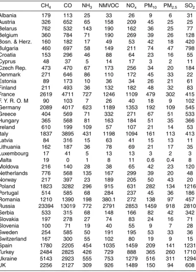
fuels, solvent use, road transport, other mobile sources, waste treatment and dis-posal, agriculture) (Table 1). According to this emission inventory UK, Spain, Ger-many, Ukraine, France and Italy have the highest NOx emissions while Ukraine, Spain and Poland have the highest SO₂ emissions (only a part of the Russian Federation and Turkey belongs to the domain examined). In general, road transport and energy

15

sector-utilities-refineries are the major sources for NOx emissions while SO2 emis-sions originate mainly from the energy sector-utilities-refineries. Emisemis-sions are pro-cessed by the Sparse Matrix Operator Kernel Emissions (SMOKE v2.6) modeling sys-tem (http://www.smoke-model.org/index.cfm) to convert their resolution to the resolu-tion needed by the air quality model using monthly, weekly and hourly time profiles

20

provided by TNO (TNO, 2011). However, TNO has reported that the temporal profiles are a generalization, not regularly updated and not country specific and could affect emissions over time for air quality modeling. The Biogenic Emission Inventory System, version 3 (BEIS3) is used for processing biogenic source emissions. Gridded land use data in 1 km resolution provided by USGS (http://edc2.usgs.gov/glcc/glcc.php), the

de-25

fault summer and winter emission factors and meteorological fields are used to create hourly model-ready biogenic emissions estimates.

(6)

ACPD

13, 6681–6705, 2013

E. Tagaris et al.

Tables Figures

◭ ◮

Back Close

Full Screen / Esc

Discussion

P

a

per

|

Dis

cussion

P

a

per

|

Discussion

P

a

per

|

Discussio

n

P

a

per

|

2006) for winter (i.e. January, 2006) and summer (i.e. July, 2006) months. CMAQ is a multipollutant, multiscale air quality model for simulating all atmospheric and land processes that affect transport, transformation, and deposition of atmospheric pollu-tants on both regional and urban scales. The modeling domain covers almost entire Europe with 177×217 grid cells of 35 km×35 km spatial resolution and 14 vertical

lay-5

ers (Fig. 1). Although a finer domain could affect modeling results studies found that it does not always enhance model performance (e.g. Queen et al., 2008). The default boundary and initial conditions for gaseous and particulate species have been used. Boundary conditions have a very minor impact on pollutants concentrations since Eu-ropean land is far away from the domain borders expect the eastern border. However,

10

due to the prevailing wind direction over Europe it does not a_ffect pollutant concentra-tions. Moreover, a spin up time of 10 days was used to wash out errors in the initial conditions. In the version used, several new pathways for secondary organic aerosol (SOA) formation have been implemented (Edney et al., 2007; Carlton et al., 2008). The CB05 is a condensed mechanism of atmospheric oxidant chemistry that provides

15

a basis for computer modeling studies of ozone, particulate matter (PM), visibility, acid deposition and air toxics issues (Yarwood et al., 2005). The core CB05 mechanism has 51 species and 156 reactions. The CB05 has been evaluated against smog cham-ber data (Jeffries et al., 2002; Carter, 2000) and the results are discussed in detail by Yarwood et al. (2005).

20

Since an extensive evaluation and discussion of meteorology used has been pre-sented by Vautard et al., (2012), here, we focus on gaseous and particulate pollutant concentrations. Briefly, Vautard et al., (2012) found that the seasonal cycle of the 10 m wind speed is well reproduced although it is overestimated over Europe. The spatial distribution of surface wind speed is fairly well simulated. Wind speed is well simulated

25

along the vertical profile but markedly overestimated at lower altitudes over Europe. It was also found that the PBL height at noon is simulated quite well. However, at 18 UTC and particularly in the summer months, the modelled PBL height is much lower than the observed. Biases of monthly means of 2 m temperature are generally small. The

(7)

ACPD

13, 6681–6705, 2013

E. Tagaris et al.

Tables Figures

◭ ◮

Back Close

Full Screen / Esc

Discussion

P

a

per

|

Dis

cussion

P

a

per

|

Discussion

P

a

per

|

Discussio

n

P

a

per

|

diurnal cycle of 2 m temperature is also fairly well reproduced while the typical verti-cal temperature profile bias is between±1 K. On average the temperature is slightly underestimated while relative humidity above the surface is overestimated.

2.2 Model evaluation

Comparison between predicted and observed gas and particle concentrations

5

is performed for January and July, 2006 using observation data from AirBase, the European air quality database (http://www.eea.europa.eu/data-and-maps/data/ airbase-the-european-air-quality-database-2). AirBase is the air quality information system maintained by the European Environment Agency (EEA) through the European topic centre on Air and Climate Change. It contains air quality data delivered annually

10

establishing a reciprocal exchange of information and data from networks and individ-ual stations measuring ambient air pollution within the Member States. Model evalua-tion is conducted, here, for species with sufficient monitoring data all over Europe such as sulfur dioxide (data from 35 countries, in our domain there are 1928 stations for winter and 1883 for summer months), nitrogen dioxide (data from 35 countries, in our

15

domain there are 2591 stations for winter and 2508 for summer months), ozone (data from 35 countries, in our domain there are 1954 stations for winter and 1977 for sum-mer months) and particulate matter <_{2.5 µm (data from 30 countries, in our domain}

there are 266 stations for winter and 267 for summer months) (Fig. 2). Unfortunately comparison with observed PM2.5components could not be performed since speciated

20

PM_2.5data are not readily available for EU; this has also recently been pointed out by other researchers (Appel et al., 2012).

2.3 E_ffect of precursor emissions

Emissions of air pollutants originated from a variety of small and large individual sources (e.g. power plants, industries, motor vehicles) varying temporally and

spa-25

(8)

ACPD

13, 6681–6705, 2013

E. Tagaris et al.

Tables Figures

◭ ◮

Back Close

Full Screen / Esc

Discussion

P

a

per

|

Dis

cussion

P

a

per

|

Discussion

P

a

per

|

Discussio

n

P

a

per

|

they are based on data sets of limited spatiotemporal coverage while countries do not always estimate emissions in a uniform and transparent manner. Assessing such uncertainties is an essential step towards the better computation of air pollutants con-centrations. In an effort to do so, here, we assess the effect of precursor emissions on air quality applying scaling factors for January and July, 2006 on NO_x, SO₂and PM_2.5

5

emissions based on the ratio Observedaverage

Predicted_average for each country. This is not just a sensitivity analysis assessing the effect of each precursor separately on air pollution since we examine the effect of the simultaneous emission change for multiple precursors on air quality. The selection of the above precursor emissions is due to the significant number of monitoring data throughout the modeling domain. Although other precursor

emis-10

sions (e.g. VOCs, NH3) affect air pollutant concentrations the limited number of their monitoring data throughout the modeling domain does not allow us to include them in the presented analysis.

3 Results and discussion

3.1 Air quality

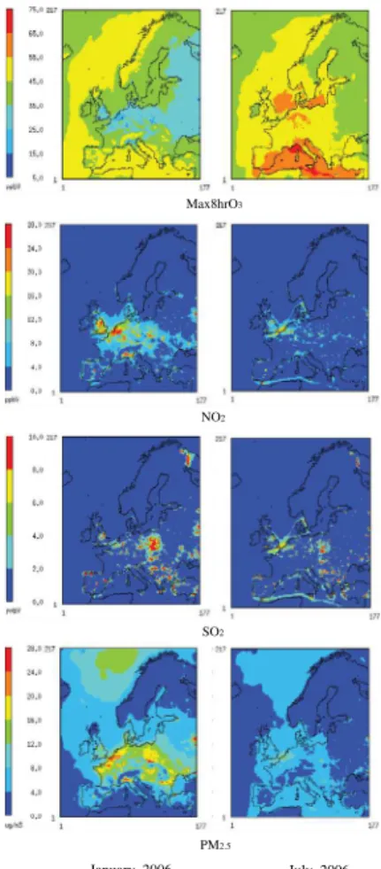
15

High ozone concentrations are illustrated in southern Europe where meteorological conditions enhance ozone production (Fig. 3). The daily average maximum 8 h ozone (Max8hrO3) concentration during July is simulated up to 75 ppbV while a big part of the domain faces concentrations higher than 50 ppbV. Higher NO2concentrations are simulated over western Europe (i.e. Belgium, the Netherlands, Germany and northern

20

France), northern Italy and UK for both seasons. Belgium and the Netherlands have elevated NO2concentrations since their small area results in a high emission rate per acre, however, they are not ranked as one of the countries with high NO_x emission rates. Road transport and industry are responsible for the elevated NOx emissions at northertn Italy while road and non-road transport energy sector and industry are

re-25

(9)

ACPD

13, 6681–6705, 2013

E. Tagaris et al.

Tables Figures

◭ ◮

Back Close

Full Screen / Esc

Discussion

P

a

per

|

Dis

cussion

P

a

per

|

Discussion

P

a

per

|

Discussio

n

P

a

per

|

January compared to July for two reasons: energy sector and industry emit more NO_x during winter and NO2photolysis is unfavorable during winter. Elevated SO2 concen-trations are simulated over eastern Europe with higher concenconcen-trations over Poland and the North Balkan Peninsula. Since power generation and industry are mainly responsi-ble for SO2emissions, SO2 concentrations are very locally depended showing higher

5

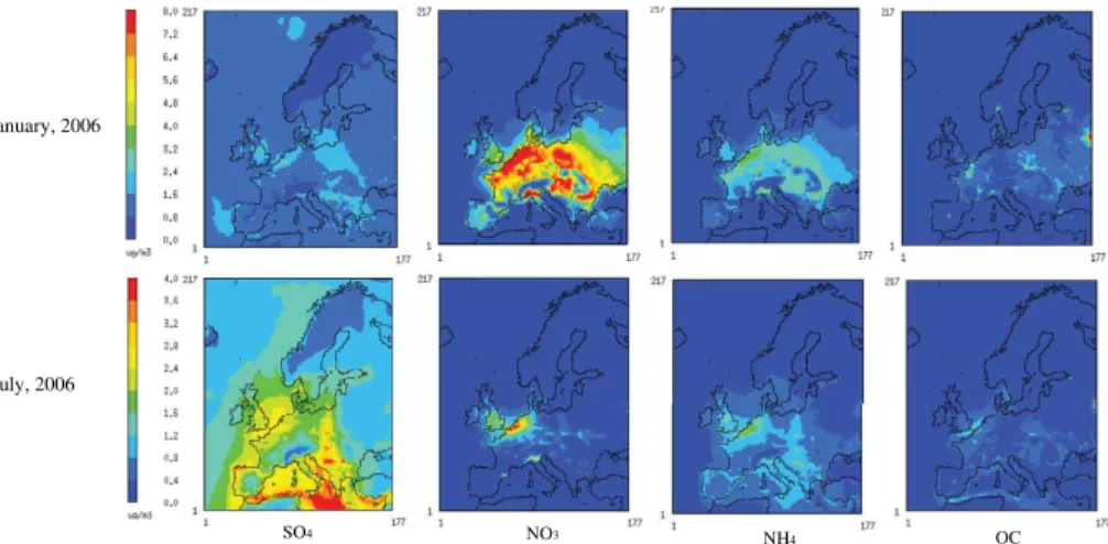
values during winter. Elevated PM2.5 levels are simulated over eastern and western Europe (i.e. up to 30 µg m−3 during winter). NO₃ is dominant during winter in western Europe and in a few eastern countries due to the high NO2 concentrations (Fig. 4). During summer NO3is dominant only in regions with elevated NH3emissions (i.e. the Netherlands and northern Italy). For the rest of the domain SO₄is dominant. Low OC

10

concentrations are simulated in general. Representation of secondary organic aerosol (SOA) formation is uncertain, and low OC has been noted in the CMAQ approaches (Foley et al., 2010). NH₄ follows SO₄ and NO₃ spatial distribution plots for both sea-sons since atmospheric SO2is oxidized to sulfuric acid which reacts with ammonia to form ammonium sulfate while gas-phase NOx, oxidizes to nitric acid which reacts with

15

ammonia to form ammonium nitrate.

Spatial distribution plots presented here for gaseous pollutants and PM2.5are similar with those presented by another study (Pay et al., 2010). Using the WRF-ARW me-teorological model, the HERMES-EMEP emission processing model, a mineral dust dynamic model (BSC-DREAM8b) and CMAQ chemical transport model they provide

20

annual simulations for 2004 over Europe.

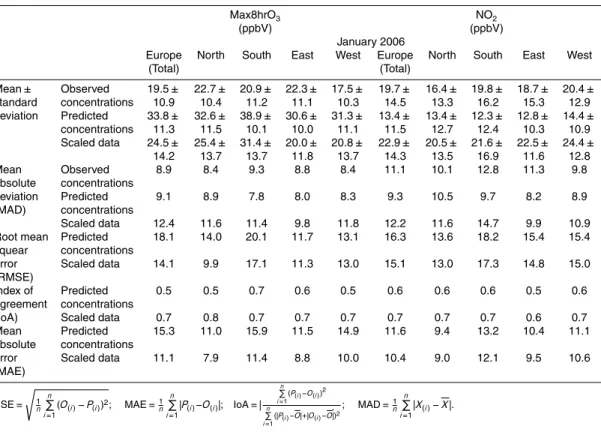
Model performance for ozone shows a mixed trend: Max8hrO3 is overpredicted for low concentrations (about 50 ppbV) while it is underpredicted for the higher ones. This trend is in agreement with the CMAQ application performed by Appel et al. (2012) for Europe where daytime ozone mixing ratio is overestimated in winter and

underesti-25

(10)

ACPD

13, 6681–6705, 2013

E. Tagaris et al.

Tables Figures

◭ ◮

Back Close

Full Screen / Esc

Discussion

P

a

per

|

Dis

cussion

P

a

per

|

Discussion

P

a

per

|

Discussio

n

P

a

per

|

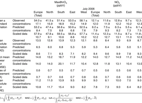
(similar simulated standard and mean absolute deviations). During summer simulated concentrations are closer to the mean simulated concentration compared to observa-tion data; this is related to the overpredicobserva-tion of the lower concentraobserva-tions. At regional scale according to the grouping used by the United Nations Statistics Department for northern, western, eastern and southern Europe (http://unstats.un.org/unsd/methods/

5

m49/m49regin.htm#europe; Fig. 1) model overestimates ozone concentrations in all regions during winter while during summer model overestimates ozone concentrations in northern and southern Europe and underestimates them in eastern and western Europe where higher concentrations have been recorded (Table 2). A consistent bias for NO2, SO2and PM2.5 estimations is noted: NO2 and PM2.5are consistently

under-10

predicted while SO₂ is consistently overpredicted for both seasons. The same biases have been also noticed by another previous study (Pay et al., 2010). The consistent un-derprediction trend for PM2.5has been found also by Appel et al. (2012) using CMAQ modeling system for Europe. At regional scale model underestimates NO₂ concentra-tions more in southern Europe and overestimates SO2concentrations more in eastern

15

Europe where higher underestimation in PM2.5concentrations is noted.

3.2 Effect of precursor emissions on air quality

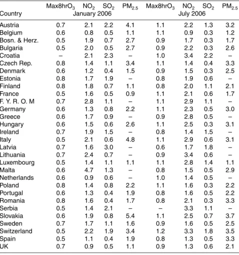
The di_fference between observed and predicted concentrations for each country based on the ratioObservedaverage

Predicted_average is presented in Table 3. This ratio for Max8hrO3is less than 1.0 during January, 2006 in all countries due to the underprediction of low ozone

concen-20

tration observed in winter. During July, 2006 the average observed concentrations are closer to the average predicted ones for all countries (this ratio is 1.0±0.1 for the ma-jority of the countries). Beside the general overprediction trend for SO2concentrations regionally over Europe, the ratio is greater than 1.0 in few countries for both seasons denoting that the average observed concentrations are higher than the average

pre-25

dicted ones for those countries. The ratio for NO2and PM2.5concentrations is almost in all countries greater than 1.0. There are numerous reasons why a bias may exist. This

(11)

ACPD

13, 6681–6705, 2013

E. Tagaris et al.

Tables Figures

◭ ◮

Back Close

Full Screen / Esc

Discussion

P

a

per

|

Dis

cussion

P

a

per

|

Discussion

P

a

per

|

Discussio

n

P

a

per

|

could be related to inaccuracies in emission inventories; a discrepancy with the me-teorological data and the source locations; topographic effects that are not accounted for in the model; or the model itself may have built in biases. To explore this, here, we examine modeling results using modified NOx, SO2and PM2.5emissions based on the ratio Observed_Predictedaverage

average for each country.

5

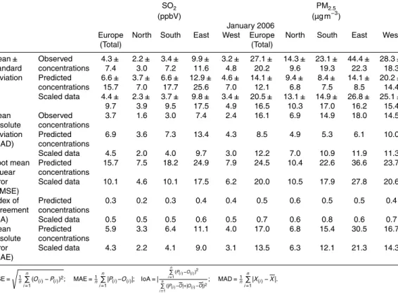
The modified emissions improve model’s performance for all examined pollutants (Table 2). Better closure is noticed for SO2 predictions. Mean simulated SO2 concen-trations using scaled emissions is similar to the mean observed concenconcen-trations while both simulated and observed values are similarly spread out around means for both seasons (i.e. similar standard deviation and mean absolutely values). Moreover all

10

statistical parameters examined here (i.e. root mean square, index of agreement and mean absolute error) are improved suggesting better model performance using scaled emissions. Statistical analysis suggests that while NO2 concentrations are better sim-ulated using scaled emissions improvement is minor compared to SO2 performance. This is attributed to the fact that scaling factors are not applied directly on NO₂ but on

15

NOx. As such NO2to NOxratio probably includes additional uncertainties that need to be investigated in the future. Standard and mean absolute deviations suggest that sim-ulated and observed values are similarly spread out around means for both seasons using scaled emissions. An improved performance is also noted for PM2.5 for both seasons. Although higher PM2.5 concentrations are simulated using scaled emissions

20

and values are spread out far away of the mean value compared to the simulations with original emissions (higher standard deviation and mean absolute error) model still underpredicts PM2.5 concentrations. This is probably related to the uncertain repre-sentation of secondary organic aerosol formation (e.g. Chen et al., 2005; Kroll et al., 2006). Better performance is also noted for Max8hrO₃ concentrations mainly during

25

winter; however, the model seems to overpredict Max8hrO3concentrations.

(12)

ACPD

13, 6681–6705, 2013

E. Tagaris et al.

Tables Figures

◭ ◮

Back Close

Full Screen / Esc

Discussion

P

a

per

|

Dis

cussion

P

a

per

|

Discussion

P

a

per

|

Discussio

n

P

a

per

|

is affected by transported pollutants from neighbor countries). However, this part of our work could suggest possible uncertainties in precursor emissions for European coun-tries although a more robust method to improve the emissions (e.g. inverse modeling on the precursor emissions) is needed for real improvements in the temporal and/or spa-tial allocation of the emissions. Assessing (i) the e_ffect of other precursor emissions,

5

(ii) the effect of a finer resolution domain, (iii) the effect of other chemical mechanism or even a different air quality model will provide more information for the role of other sources of uncertainty.

4 Conclusions

Application of CMAQ modeling system over Europe for January and July, 2006

us-10

ing the TNO gridded anthropogenic emissions database for the year 2006 shows an overprediction trend for low ozone concentrations (less than 50 ppbV) while it is under-predicted for the higher ones, although spatial distributions are reasonably estimated (e.g. higher ozone concentrations in southern Europe). Simulated concentrations for NO2, SO2 and PM2.5 suggest a consistent bias: SO2 is overpredicted while NO2 and

15

PM2.5 are underpredicted. Speciated PM2.5 components give low OC concentrations as a result of the uncertain representation of SOA formation. Assessing the di_fference between observed and predicted concentrations for each country and scaling the emis-sions based on that seems to statistically enhance model performance (i.e. root mean square, index of agreement and mean absolute error are improved). Although a

num-20

ber of reasons could affect model performance (e.g. meteorological data, topographic effects or the model itself), results from the current study could suggest possible un-certainties in precursor emissions for the European countries.

(13)

ACPD

13, 6681–6705, 2013

E. Tagaris et al.

Tables Figures

◭ ◮

Back Close

Full Screen / Esc

Discussion

P

a

per

|

Dis

cussion

P

a

per

|

Discussion

P

a

per

|

Discussio

n

P

a

per

|

Supplementary material related to this article is available online at: http://www.atmos-chem-phys-discuss.net/13/6681/2013/

acpd-13-6681-2013-supplement.pdf.

Acknowledgements. This work was supported by the FP7-REGPOT-2008-1 grant No. 229773 and the National Strategic Reference Framework (NSRF) 2007–2013 grand No

09SYN-31-5

667. We gratefully acknowledge the first Air Quality Model Evaluation International Initiative (AQMEII) activity. The following agencies have prepared the databases used in the study: TNO (European emissions processing), Laboratoire des Sciences du Climat et de l’Environment, IPSL, CEA/CNRS/UVSQ (gridded meteorology for Europe).

References

10

Appel, K. W., Chemel, C., Roselle, S. J., Francis, X. V., Hu, R. M., Sokhi, R. S., Rao, S. T., and Galmarini, S.: Examination of the Community Multiscale Air Quality (CMAQ) model per-formance over the north American and European domains, Atmos. Environ., 53, 142–145, 2012.

Basart, S., Pay, M. T., Jorba, O., P ´erez, C., Jim ´enez-Guerrero, P., Schulz, M., and

Bal-15

dasano, J. M.: Aerosols in the CALIOPE air quality modelling system: evaluation and analysis of PM levels, optical depths and chemical composition over Europe, Atmos. Chem. Phys., 12, 3363–3392, doi:10.5194/acp-12-3363-2012, 2012.

Byun, D. W. and Schere, K. L.: Review of the governing equations, computational algorithms, and other components of the Models-3 Community Multscale Air Quality (CMAQ) modeling

20

system, Appl. Mech. Rev., 59, 51–77, 2006.

Byun, D. W., Pleim, J. E., Tang, R. T., and Bourgeois, A.: Meteorology-Chemistry Interface Pro-cessor (MCIP) for Models-3 Community Multiscale Air Quality (CMAQ) Modeling System, in: Science algorithms of the EPA Models-3 Community Multiscale Air Quality (CMAQ) Modeling System, US Environmental Protection Agency Report, EPA-600/R-99/030, US EPA, Office

25

of Research and Development, Washington, DC, 12-1–12-91, 1999.

(14)

ACPD

13, 6681–6705, 2013

E. Tagaris et al.

Tables Figures

◭ ◮

Back Close

Full Screen / Esc

Discussion

P

a

per

|

Dis

cussion

P

a

per

|

Discussion

P

a

per

|

Discussio

n

P

a

per

|

is included: comparisons of organic carbon predictions with measurements, Environ. Sci. Technol., 42, 8798–8802, 2008.

Carter, W. P. L.: Programs and Files Implementing the SAPRC-99 Mechanism and its Associ-ated Emissions Processing Procedures for Models-3 and Other Regional Models, Report to the US EPA, available at: www.cert.ucr.edu/∼_{carter/pubs/s99mod3.pdf (last access: March}

5

2013), 2000.

Chen, J. and Griffin, R. J.: Modeling secondary organic aerosol formation from oxidation of a-pinene, b-pinene, and d-limonene, Atmos. Environ., 39, 7731–7744, 2005.

Edney, E. O., Kleindienst, T. E., Lewandowski, M., Offenberg, J. H.: Updated SOA chemical mechanism for the Community Multi-Scale Air Quality model, EPA 600/X-07/025, US EPA,

10

Research Triangle Park, NC, 2007.

Foley, K. M., Roselle, S. J., Appel, K. W., Bhave, P. V., Pleim, J. E., Otte, T. L., Mathur, R., Sar-war, G., Young, J. O., Gilliam, R. C., Nolte, C. G., Kelly, J. T., Gilliland, A. B., and Bash, J. O.: Incremental testing of the Community Multiscale Air Quality (CMAQ) modeling system ver-sion 4.7, Geosci. Model Dev., 3, 205–226, doi:10.5194/gmd-3-205-2010, 2010.

15

Grell, G., Dudhia, J., and Stauffer, D. R.: A description of the fifth generation Penn State/NCAR mesoscale model (MM5), NCAR Tech. Note, NCAR/TN-398+STR, Natl. Cent. for Atmos. Res., Boulder, Colorado, 1994.

Jeffries, H. E., Voicu, I., and Sexton, K.: Experimental Tests of Reactivity and Reevaluation of The Carbon Bond Four Photochemical Reaction Mechanism, final report for Cooperative

20

Agreement No. R828906, US EPA, RTP, NC, 2002.

Jonson, J. E., Simpson, D., Fagerli, H., and Solberg, S.: Can we explain the trends in European ozone levels?, Atmos. Chem. Phys., 6, 51–66, doi:10.5194/acp-6-51-2006, 2006.

Kroll, J. H., Ng, N. L., Murphy, S. M., Flagan, R. C., and Seinfeld, J. H.: Secondary organic aerosol formation from isoprene photooxidation, Environ. Sci. Technol., 40, 1869–1877,

25

2006.

Langmann, B., Varghese, S., Marmer, E., Vignati, E., Wilson, J., Stier, P., and O’Dowd, C.: Aerosol distribution over Europe: a model evaluation study with detailed aerosol micro-physics, Atmos. Chem. Phys., 8, 1591–1607, doi:10.5194/acp-8-1591-2008, 2008.

Nopmongcol, U., Koo, B., Tai, E., Jung, J., Piyachaturawat, P., Emery, C., Yarwood, G.,

30

Pirovano, G., Mitsakou, C., and Kallos, G.: Modeling Europe with CAMx for the Air Qual-ity Model Evaluation International Initiative (AQMEII), Atmos. Environ., 53, 177–185, 2012.

(15)

ACPD

13, 6681–6705, 2013

E. Tagaris et al.

Tables Figures

◭ ◮

Back Close

Full Screen / Esc

Discussion

P

a

per

|

Dis

cussion

P

a

per

|

Discussion

P

a

per

|

Discussio

n

P

a

per

|

Pay, M. T., Piot, M., Jorba, O., Gass ó, S., Gonçalves, M., Basart, S., Dabdub, D., Jim énez-Guerrero, P., and Baldasano, J. M.: A full year evaluation of the CALIOPE-EU air quality modeling system over Europe for 2004, Atmos. Environ., 44, 3322–3342, 2010.

Peng, R. D., Dominici, F., Pastor-Barriuso, R., Zeger, S. L., and Samet, J. M.: Seasonal analyses of air pollution and mortality in 100 US cities, Am. J. Epidemiol., 161, 585–594, 2005.

5

Queen, A. and Zang, Y.: Examining the sensitivity of MM5–CMAQ predictions to explicit mi-crophysics schemes and horizontal grid resolutions, Part III – the impact of horizontal grid resolution, Atmos. Environ., 42, 3869–3881, 2008.

Sartelet, K. N., Debry, E., Fahey, K., Roustan, Y., Tombette, M., and Sportisse, B.: Simulation of aerosols and gas-phase species over Europe with the POLYPHEMUS system, Part I –

10

model-to-data comparison for 2001, Atmos. Environ., 41, 6116–6131, 2007.

Seinfeld, J. and Pandis, S. N.: Atmospheric Chemistry and Physics, John Wiley, Hoboken, NJ, USA, 2006.

Simpson, D., Yttri, K. E., Klimont, Z., Kupiainen, K., Caseiro, A., Gelencseır, A., Pio, C., Puxbaum, H., and Legrand, M.: Modeling carbonaceous aerosol over Europe:

analy-15

sis of the CARBOSOL and EMEP EC/OC campaigns, J. Geophys. Res., 112, D23S14, doi:10.1029/2006JD008158, 2007.

TNO: Description of current temporal emission patterns and sensitivity of predicted AQ for tem-poral emission patterns, TNO Report, TNO, Princetonlaan 6, 3584 CB Utrecht, the Nether-lands, 2011.

20

Vautard, R., Moran, M. D., Solazzo, E., Gilliam, R. C., Matthias, V., Bianconi, R., Chemel, C., Ferreira, J., Geyer, B., Hansen, A. B., Jericevic, A., Prank, M., Segers, A., Silver, J. D., Wer-hahn, J., Wolke, R., Rao, S. T., and Galmarini, S.: Evaluation of the meteorological forcing used for the Air Quality Model Evaluation International Initiative (AQMEII) air quality simula-tions, Atmos. Environ., 53, 15–37, 2012.

25

(16)

ACPD

13, 6681–6705, 2013

E. Tagaris et al.

Tables Figures

◭ ◮

Back Close

Full Screen / Esc

Discussion

P

a

per

|

Dis

cussion

P

a

per

|

Discussion

P

a

per

|

Discussio

n

P

a

per

|

Table 1.Emissions (kt yr−1).

CH₄ CO NH₃ NMVOC NO_x PM₁₀ PM_2.5 SO₂

Albania 179 113 25 33 26 9 6 31

Austria 326 652 65 158 209 45 25 25

Belarus 762 532 143 190 162 36 25 77

Belgium 360 784 71 190 269 39 26 128

Bosn. & Herz. 160 182 17 49 53 42 18 420

Bulgaria 460 697 58 149 211 74 47 798

Croatia 153 296 46 88 64 23 16 55

Cyprus 48 37 5 14 17 3 2 11

Czech Rep. 473 470 67 173 256 34 20 184

Denmark 271 646 86 110 172 45 33 22

Estonia 89 173 10 36 34 26 21 61

Finland 211 493 36 132 182 48 32 83

France 2619 4711 727 1246 1109 479 302 415

F. Y. R. O. M 90 103 7 26 40 18 9 102

Germany 2089 4017 623 1189 1353 192 109 545

Greece 404 569 71 332 271 67 51 533

Hungary 365 568 81 163 184 51 35 366

Ireland 610 199 109 57 107 21 14 53

Italy 1837 3895 431 1198 1094 161 113 413

Latvia 84 316 15 63 41 15 13 11

Lithuania 162 187 36 78 69 21 17 35

Luxembourg 17 41 5 13 13 3 2 3

Malta 19 0 1 8 11 0.6 0.4 8

Moldova 216 140 28 38 65 42 23 120

Netherlands 776 568 135 167 299 39 20 48

Norway 217 397 23 189 205 50 43 20

Poland 1823 3282 296 915 631 282 134 1216

Portugal 514 585 68 284 237 45 36 186

Romania 1210 1390 198 380.1 272 138 97 457 Russia 23394 13019 772 2791 2853 1459 918 2810

Serbia 533 315 68 148 166 82 42 342

Slovakia 197 278 27 74 83 24 16 71

Slovenia 100 71 19 40 55 9 7 28

Sweden 254 585 50 191 195 53 33 36

Switzerland 167 300 55 102 80 19 9 15

Spain 1780 2205 454 1035 1459 209 141 1231 Turkey 2484 2825 426 729 888 365 260 1710 Ukraine 5143 2923 555 753 1279 516 311 1294

UK 2256 2127 309 926 1489 150 94 608

(17)

ACPD

13, 6681–6705, 2013

E. Tagaris et al.

Tables Figures

◭ ◮

Back Close

Full Screen / Esc

Discussion

P

a

per

|

Dis

cussion

P

a

per

|

Discussion

P

a

per

|

Discussio

n

P

a

per

|

Table 2.Statistical analysis for hourly average NO₂and SO₂concentrations and daily average Max8hrO₃and PM_2.5concentrations over Europe.

Max8hrO₃ NO₂

(ppbV) (ppbV)

January 2006

Europe North South East West Europe North South East West

(Total) (Total)

Mean± Observed 19.5± 22.7± 20.9± 22.3± 17.5± 19.7± 16.4± 19.8± 18.7± 20.4± standard concentrations 10.9 10.4 11.2 11.1 10.3 14.5 13.3 16.2 15.3 12.9 deviation Predicted 33.8± 32.6± 38.9± 30.6± 31.3± 13.4± 13.4± 12.3± 12.8± 14.4±

concentrations 11.3 11.5 10.1 10.0 11.1 11.5 12.7 12.4 10.3 10.9 Scaled data 24.5± 25.4± 31.4± 20.0± 20.8± 22.9± 20.5± 21.6± 22.5± 24.4±

14.2 13.7 13.7 11.8 13.7 14.3 13.5 16.9 11.6 12.8

Mean Observed 8.9 8.4 9.3 8.8 8.4 11.1 10.1 12.8 11.3 9.8

absolute concentrations

deviation Predicted 9.1 8.9 7.8 8.0 8.3 9.3 10.5 9.7 8.2 8.9 (MAD) concentrations

Scaled data 12.4 11.6 11.4 9.8 11.8 12.2 11.6 14.7 9.9 10.9 Root mean Predicted 18.1 14.0 20.1 11.7 13.1 16.3 13.6 18.2 15.4 15.4 squear concentrations

error Scaled data 14.1 9.9 17.1 11.3 13.0 15.1 13.0 17.3 14.8 15.0 (RMSE)

Index of Predicted 0.5 0.5 0.7 0.6 0.5 0.6 0.6 0.6 0.5 0.6

agreement concentrations

(IoA) Scaled data 0.7 0.8 0.7 0.7 0.7 0.7 0.7 0.7 0.6 0.7

Mean Predicted 15.3 11.0 15.9 11.5 14.9 11.6 9.4 13.2 10.4 11.1 absolute concentrations

error Scaled data 11.1 7.9 11.4 8.8 10.0 10.4 9.0 12.1 9.5 10.6 (MAE)

RMSE=

s 1 n n P

i=1

(O₍_i₎−P₍_i₎)2_; _MAE₌1 n n P

i=1

|P₍_i₎−O₍_i₎|; IoA=| n

P

i=1 (P₍i)−O(i))2

n

P

i=1

(|P₍i)−O|+|O(i)−O|)2

; MAD=1n

n P

i=1

(18)

ACPD

13, 6681–6705, 2013

E. Tagaris et al.

Tables Figures

◭ ◮

Back Close

Full Screen / Esc

Discussion

P

a

per

|

Dis

cussion

P

a

per

|

Discussion

P

a

per

|

Discussio

n

P

a

per

|

Table 2.Continued.

Max8hrO3 NO2

(ppbV) (ppbV)

July 2006

(Total) (Total)

Mean± Observed 54.0± 41.5± 51.4± 53.0± 58.1± 12.1± 11.6± 12.8± 9.7± 12.3± standard concentrations 17.1 15.9 18.9 15.2 14.9 12.0 11.9 12.2 10.2 12.3 deviation Predicted 53.2± 47.4± 56.8± 50.6± 52.5± 6.2± 7.5± 6.3± 5.5± 6.1± concentrations 8.4 7.5 8.8 6.8 7.6 7.9 9.3 8.2 7.3 7.5 Scaled data 57.9± 47.8± 59.5± 56.8± 57.7± 11.4± 12.3± 11.5± 8.7± 11.8±

10.7 9.1 10.6 8.8 10.2 12.2 12.7 13.1 11.0 12.5

Mean Observed 13.5 12.6 13.9 12.3 12.1 8.6 8.4 9.0 6.9 8.7

Scaled data 8.6 7.1 8.3 7.1 8.2 9.4 9.6 9.9 7.8 9.3

Root mean Predicted 14.6 13.2 18.7 11.9 12.2 14.0 12.7 14.9 11.2 14.2 squear concentrations

Index of Predicted 0.6 0.7 0.5 0.7 0.7 0.5 0.6 0.5 0.6 0.5

agreement concentrations

(IoA) Scaled data 0.7 0.7 0.6 0.7 0.8 0.6 0.7 0.6 0.6 0.6

Mean Predicted 11.2 11.0 13.9 9.5 9.9 9.0 8.1 10.0 7.0 9.0

RMSE=

s 1

n n

P

i=1

(O₍i)−P(i))2; MAE=1n n

P

i=1

|P₍i)−O(i)|; IoA=| n P

i=1 (P₍i)−O(i))2

n P

i=1

(|P(i)−O|+|O(i)−O|)2

; MAD=1

n n

P

i=1 |X₍i)−X|.

(19)

ACPD

13, 6681–6705, 2013

E. Tagaris et al.

Tables Figures

◭ ◮

Back Close

Full Screen / Esc

Discussion

P

a

per

|

Dis

cussion

P

a

per

|

Discussion

P

a

per

|

Discussio

n

P

a

per

|

SO2 PM2.5

(ppbV) (µg m−3)

January 2006

(Total) (Total)

9.7 3.9 9.5 17.5 4.9 16.5 10.3 17.0 16.2 15.4

Mean Observed 3.7 1.6 3.0 7.4 2.4 16.1 6.9 14.9 18.0 14.5

Index of Predicted 0.3 0.2 0.3 0.4 0.4 0.5 0.6 0.5 0.5 0.4 agreement concentrations

(IoA) Scaled data 0.5 0.5 0.5 0.6 0.5 0.7 0.6 0.8 0.6 0.7

Mean Predicted 5.9 3.3 6.4 11.1 4.0 17.0 6.8 15.4 30.5 16.7 absolute concentrations

RMSE=

s 1

n n

P

i=1

P

i=1

i=1 (P(i)−O(i))2 n P

i=1

(|P(i)−O|+|O(i)−O|)2

; MAD=1

n n

P

(20)

ACPD

13, 6681–6705, 2013

E. Tagaris et al.

Tables Figures

◭ ◮

Back Close

Full Screen / Esc

Discussion

P

a

per

|

Dis

cussion

P

a

per

|

Discussion

P

a

per

|

Discussio

n

P

a

per

|

SO2 PM2.5

(ppbV) (µg m−3)

July 2006

(Total) (Total)

4.8 3.3 5.8 4.8 4.0 6.3 5.1 6.0 5.4 6.9

Mean Observed 1.9 1.5 2.2 1.7 1.6 5.9 5.7 6.4 7.4 4.5

Index of Predicted 0.3 0.3 0.3 0.2 0.3 0.4 0.5 0.5 0.5 0.4 agreement concentrations

(IoA) Scaled data 0.6 0.5 0.5 0.6 0.6 0.6 0.7 0.6 0.6 0.5 Mean Predicted 4.2 2.6 4.6 6.4 3.1 10.1 7.2 11.4 13.3 8.6 absolute concentrations

RMSE=

s 1

n n

P

i=1

P

i=1

i=1 (P(i)−O(i))2 n P

i=1

(|P(i)−O|+|O(i)−O|)2

; MAD=1

n n

P

i=1 |X₍i)−X|.

(21)

ACPD

13, 6681–6705, 2013

E. Tagaris et al.

Tables Figures

◭ ◮

Back Close

Full Screen / Esc

Discussion

P

a

per

|

Dis

cussion

P

a

per

|

Discussion

P

a

per

|

Discussio

n

P

a

per

|

Table 3.Observed_avergae/Predicted_averageconcentrations for the European countries.

Max8hrO₃ NO₂ SO₂ PM_2.5 Max8hrO₃ NO₂ SO₂ PM_2.5

Country January 2006 July 2006

Austria 0.7 2.1 2.2 4.1 1.1 2.2 1.3 3.2

Belgium 0.6 0.8 0.5 1.1 1.1 0.9 0.3 1.2

Bosn. & Herz. 0.5 1.9 0.7 2.7 0.9 1.7 0.3 1.7

Bulgaria 0.5 2.0 0.5 2.7 0.9 2.2 0.3 2.6

Croatia – 2.1 2.3 – 1.0 3.4 2.2 –

Czech Rep. 0.8 1.4 1.1 3.4 1.1 1.4 0.4 3.3

Denmark 0.6 1.2 0.4 1.5 0.9 1.5 0.3 2.5

Estonia 0.8 1.7 1.9 – 0.8 1.9 0.6 –

Finland 0.8 1.8 0.7 1.1 0.8 2.0 1.1 2.1

France 0.5 1.6 0.5 0.9 1.1 2.1 0.6 1.7

F. Y. R. O. M 0.7 2.8 1.1 – 1.1 2.9 1.1 –

Germany 0.6 1.3 0.8 2.2 1.1 2.3 0.5 3.0

Greece 0.6 1.7 0.9 – 0.9 2.8 0.5 –

Hungary 0.6 1.5 0.6 2.6 1.1 2.5 0.3 3.1

Ireland 0.7 1.9 1.5 – 0.8 1.4 1.5 –

Italy 0.5 2.1 0.6 4.8 1.1 2.9 0.6 3.1

Latvia 0.7 1.6 3.0 – 0.6 1.7 1.8 –

Lithuania 0.7 2.4 0.7 – 0.9 3.4 0.6 –

Luxembourg 0.5 1.4 1.1 1.1 1.1 2.8 1.4 1.1

Malta 0.6 4.7 1.3 – 0.8 1.5 0.5 2.9

Netherlands 0.6 0.9 0.6 – 1.0 1.4 0.5 –

Poland 0.8 1.4 0.8 2.2 1.1 1.6 0.3 2.2

Portugal 0.6 1.3 0.4 1.9 0.8 1.6 0.5 2.2

Romania 0.8 1.6 0.4 1.7 0.8 2.1 0.3 3.3

Serbia 0.5 1.4 2.1 – – 3.3 1.1 –

Slovakia 0.6 1.9 0.8 5.4 1.1 2.5 0.7 3.7

Sweden 0.7 1.7 1.1 1.6 0.9 1.6 0.5 2.5

Switzerland 0.5 2.2 1.9 3.4 1.2 3.3 1.8 3.5

Spain 0.5 1.1 0.4 1.9 0.8 1.3 0.5 3.3

(22)

ACPD

13, 6681–6705, 2013

E. Tagaris et al.

Tables Figures

◭ ◮

Back Close

Full Screen / Esc

Discussion

P

a

per

|

Dis

cussion

P

a

per

|

Discussion

P

a

per

|

Discussio

n

P

a

per

|

Fig. 1.Modeling domain and the regional European grouping used by the United Nations Statis-tics Department.

(23)

ACPD

13, 6681–6705, 2013

E. Tagaris et al.

Tables Figures

◭ ◮

Back Close

Full Screen / Esc

Discussion

P

a

per

|

Dis

cussion

P

a

per

|

Discussion

P

a

per

|

Discussio

n

P

a

per

|

O3 monitoring stations NO2monitoring stations

SO2 monitoring stations PM2.5monitoring stations

(24)

ACPD

13, 6681–6705, 2013

E. Tagaris et al.

Tables Figures

◭ ◮

Back Close

Full Screen / Esc

Discussion

P

a

per

|

Dis

cussion

P

a

per

|

Discussion

P

a

per

|

Discussio

n

P

a

per

|

Max8hrO3

January, 2006 July, 2006

NO2

SO2

PM2.5 SO2

Fig. 3.Simulated daily (Max8hrO₃, PM_2.5) and hourly (NO₂, SO₂) average concentrations for January (left column) and July (right column) 2006.

(25)

ACPD

13, 6681–6705, 2013

E. Tagaris et al.

Tables Figures

◭ ◮

Back Close

Full Screen / Esc

Discussion

P

a

per

|

Dis

cussion

P

a

per

|

Discussion

P

a

per

|

Discussio

n

P

a

per

|

NO3 _NH4 OC

SO4

January, 2006

July, 2006