GMDD
6, 1599–1688, 2013PEATBOG
Y. Wu and C. Blodau
Title Page
Abstract Introduction
Conclusions References
Tables Figures
◭ ◮
◭ ◮
Back Close
Full Screen / Esc
Printer-friendly Version
Interactive Discussion
Discussion
P
a
per
|
Dis
cussion
P
a
per
|
Discussion
P
a
per
|
Discussio
n
P
a
per
|
Geosci. Model Dev. Discuss., 6, 1599–1688, 2013 www.geosci-model-dev-discuss.net/6/1599/2013/ doi:10.5194/gmdd-6-1599-2013
© Author(s) 2013. CC Attribution 3.0 License.
Geoscientiic Geoscientiic
Geoscientiic
Open Access
Geoscientiic
Model Development
Discussions
This discussion paper is/has been under review for the journal Geoscientific Model Development (GMD). Please refer to the corresponding final paper in GMD if available.
PEATBOG: a biogeochemical model for
analyzing coupled carbon and nitrogen
dynamics in northern peatlands
Y. Wu and C. Blodau
Hydrology Group, Institute of Landscape Ecology, FB 14 Geosciences, University of M ¨unster, Germany, Heisenbergstraße 2, 48149 M ¨unster, Germany
Received: 14 November 2012 – Accepted: 12 February 2013 – Published: 4 March 2013
Correspondence to: C. Blodau ([email protected])
GMDD
6, 1599–1688, 2013PEATBOG
Y. Wu and C. Blodau
Title Page
Abstract Introduction
Conclusions References
Tables Figures
◭ ◮
◭ ◮
Back Close
Full Screen / Esc
Printer-friendly Version
Interactive Discussion
Discussion
P
a
per
|
Dis
cussion
P
a
per
|
Discussion
P
a
per
|
Discussio
n
P
a
per
|
Abstract
Elevated nitrogen deposition and climate change alter the vegetation communities and carbon (C) and nitrogen (N) cycling in peatlands. To address this issue we developed a new process-oriented biogeochemical model (PEATBOG) for analyzing coupled carbon and nitrogen dynamics in northern peatlands. The model consists of four submodels,
5
which simulate: (1) daily water table depth and depth profiles of soil moisture, temper-ature and oxygen levels; (2) competition among three plants functional types (PFTs), production and litter production of plants; (3) decomposition of peat; and (4) produc-tion, consumpproduc-tion, diffusion and export of dissolved C and N species in soil water. The model is novel in the integration of the C and N cycles, the explicit spatial resolution
10
belowground, the consistent conceptualization of movement of water and solutes, the incorporation of stoichiometric controls on elemental fluxes and a consistent concep-tualization of C and N reactivity in vegetation and soil organic matter. The model was evaluated for the Mer Bleue Bog, near Ottawa, Ontario, with regards to simulation of soil moisture and temperature and the most important processes in the C and N cycles.
15
Model sensitivity was tested for nitrogen input, precipitation, and temperature, and the choices of the most uncertain parameters were justified. A simulation of nitrogen de-position over 40 yr demonstrates the advantages of the PEATBOG model in tracking biogeochemical effects and vegetation change in the ecosystem.
1 Introduction
20
Peatlands represent the largest terrestrial soil C pool and a significant N pool. Globally, peat stores about 547 PgC (Yu et al., 2010) and 8 to 15 Pg N, accounting for one third of the terrestrial C and 9 % to 16 % of the soil organic N storage (Wieder and Vitt, 2006). Northern peatlands have accumulated 16 to 23 g C m−2yr−1throughout the Holocene and 0.42 g N m−2yr−1in the past 1000 yr on average (Vitt et al., 2000; Turunen et al.,
25
GMDD
6, 1599–1688, 2013PEATBOG
Y. Wu and C. Blodau
Title Page
Abstract Introduction
Conclusions References
Tables Figures
◭ ◮
◭ ◮
Back Close
Full Screen / Esc
Printer-friendly Version
Interactive Discussion
Discussion
P
a
per
|
Dis
cussion
P
a
per
|
Discussion
P
a
per
|
Discussio
n
P
a
per
|
has been primarily attributed to low decomposition rates, which compensate for the low production in comparison to other ecosystems (Coulson and Butterfield, 1978; Clymo, 1984). The two characteristic environmental conditions in northern peatlands-high wa-ter table (WT) and low temperature, play an essential role in preserving the large C pool by impeding material translocation and transformation in the permanently saturated
5
zone (Clymo, 1984). Although the total N storage in peat is substantial, the scarcity of biologically available N induces a conservative manner of N cycling in peatlands (Ross-wall and Granhall, 1980; Urban et al., 1988).Sphagnummosses are highly adapted to the nutrient poor environment and successfully compete with vascular plants through a series of competition strategies, such as inception of N that is deposited from the
10
atmosphere, internal recycling of N, and a minimized N release from litter with low decomposability (Damman, 1988; Aldous, 2002).
Climate change and elevated N deposition are likely to alter the structure and func-tioning of peatlands through interactive ways that are incompletely understood. In gen-eral, drought and a warmer environment were found to affect vegetation composition by
15
suppressingSphagnummosses and promoting vascular plants (Weltzin et al., 2003),
which in turn alters litter quality, C and N mineralization rates (Keller et al., 2004; Bay-ley et al., 2005; Breeuwer et al., 2008), and the C and N balance (Moore et al., 1998; Malmer et al., 2005). In northern peatlands, nitrogen is often a limiting nutrient and reg-ulates the rates of C and N cycling and individual processes, and thus also controls
ele-20
mental effluxes to the atmosphere and discharging streams. Excessive N entering peat-lands could induce changes in various processes that may lead to non-linear and even contrasting consequences with respect to C and N budgets, especially on longer time scales. For example, experimentally added N was found to increase photosynthetic ca-pacity and growth of severalSphagnumspecies up to ca. 1.5 g N m−2yr−1before
caus-25
GMDD
6, 1599–1688, 2013PEATBOG
Y. Wu and C. Blodau
Title Page
Abstract Introduction
Conclusions References
Tables Figures
◭ ◮
◭ ◮
Back Close
Full Screen / Esc
Printer-friendly Version
Interactive Discussion
Discussion
P
a
per
|
Dis
cussion
P
a
per
|
Discussion
P
a
per
|
Discussio
n
P
a
per
|
N deposition gradients ranging from 0.2 to 2 g N m−2yr−1demonstrated a relation be-tween N deposition and litter decomposition rates (Bragazza et al., 2006), in addition the effects seemed to depend on litter quality (Bragazza et al., 2009; Currey et al., 2009) and deposited N forms (Currey et al., 2010). In both long-term N fertilization experiments and survey studies an increase in N content in the surface peat and in
5
the soil water was observed at the high N sites (Xing et al., 2010) but enhanced N ef-fluxes in form of N2O remained elusive (Bubier et al., 2007). In contrast, N2O emission was found in short-term N and P fertilization experiments (Lund et al., 2009). Labora-tory and field experiments aiming to quantify the combined effects of temperature, WT and N elevation have thus often arrived at contradictory conclusions, due to the
inter-10
play of effects in time and space (Norby et al., 2001; Breeuwer et al., 2008; Robroek et al., 2009). Furthermore, elevated N deposition was recently suggested to affect soil temperature and moisture through changes in the vegetation community with potential feedbacks on elemental cycles (Wendel et al., 2011).
Ecosystem modeling has become an important approach in analyzing the interacting
15
effects of climate and N deposition on peatlands and in making long-term predictions; examples are provided by PCARS (Frolking et al., 2002),ecosys(Dimitrov et al., 2011), Wetland-DNDC (Zhang, 2002), and MWM (St-Hilaire et al., 2010). While models have been thoroughly developed to investigate peatland C cycling (e.g. PCARS, MWM), there have been few attempts to integrate N cycling in peatland models, although N
20
is mostly considered to be the limiting factor on primary production (Heijmans et al., 2008). In the mentioned models, N is generally passively bound to C pools by C/N ratios, while active nitrogen transformation and translocation among N pools is omitted. To make progress towards closing this gap, we present a novel model for the analysis of the coupled C and N cycles in northern peatlands. The model is designed to fulfill the
25
GMDD
6, 1599–1688, 2013PEATBOG
Y. Wu and C. Blodau
Title Page
Abstract Introduction
Conclusions References
Tables Figures
◭ ◮
◭ ◮
Back Close
Full Screen / Esc
Printer-friendly Version
Interactive Discussion
Discussion
P
a
per
|
Dis
cussion
P
a
per
|
Discussion
P
a
per
|
Discussio
n
P
a
per
|
and climate change; and (5) to predict the combined impact of elevated N deposition and climate change on peatland C and N cycling.
In this paper, we focus on the integration of C and N cycling through vegetation, soil organic matter and soil water, the coupling of C and N throughout the ecosystem, and the consistency of mass movements between pools. We first highlight the structural
5
design and principles that governed the modeling process, and then explain the com-ponents of the model by focusing on the individual submodels. To improve readability of the text the equations are listed in Appendix A. We subsequently present an eval-uation of the simulated WT dynamics, C fluxes, depth profiles of CO2and CH4 in soil water, and C and N budgets. The model output is compared against observations for
10
the well characterized Mer Bleue Bog (MB), Ontario, Canada. We also present sen-sitivity analyses for environmental controls, such as temperature, precipitation, and N deposition, and for some calibrated key parameters. Finally we demonstrate the poten-tial of the model for analyzing the effects of experimental long-term N deposition and climate change.
15
2 Model description
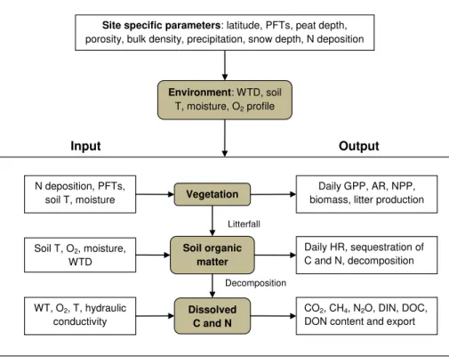
The PEATBOG (Pollution, Precipitation and Temperature impacts on peatland Biodi-versity and Biogeochemistry; see acknowledgements) model version 1.0 was imple-mented in Stella®and integrates four submodels:environment,vegetation,soil organic matter (SOM),dissolved C and N(Fig. 1). Theenvironmentsubmodel generates daily
20
WT depth from a modified mixed mire water and heat (MMWH) model (Granberg et al., 1999) and depth profiles of soil moisture, peat temperature and oxygen concentration. Thevegetationsubmodel simulates the C and N flows and the competition for light and nutrients among three plant functional types (PFTs): mosses, graminoids and shrubs. Most of the algorithms of plant physiology were adopted from the Hurley pasture (HPM)
25
GMDD
6, 1599–1688, 2013PEATBOG
Y. Wu and C. Blodau
Title Page
Abstract Introduction
Conclusions References
Tables Figures
◭ ◮
◭ ◮
Back Close
Full Screen / Esc
Printer-friendly Version
Interactive Discussion
Discussion
P
a
per
|
Dis
cussion
P
a
per
|
Discussion
P
a
per
|
Discussio
n
P
a
per
|
environment. Litter and exudates from thevegetationsubmodel flow into theSOM
sub-model and are decomposed into dissolved C and N. Thedissolved C and N submodel
tracks the fate of dissolved C and N as DOC, CH4, CO2 and DON, NH+4, and NO−3. The model does not consider hummock-hollow microtopography of peatlands, which in other studies had no statistically significant effect when simulating ecosystem level
5
CO2exchange (Wu et al., 2011).
2.1 Model structure and principles
The following three principles were imbedded in the model in terms of scale, resolution and structure:
2.1.1 High spatial and moderate temporal resolution
10
In comparison to other biogeochemical process models of peatland C cycling (Frolking et al., 2002; St-Hilaire et al., 2010) that primarily focus on the ecosystem-atmosphere interactions, we increased the spatial representation and kept the temporal resolution fairly low. We divided the belowground peat into 20 layers (i) with a vertical resolution of 5 cm except for an unconfined bottom layer. This structure applies to all belowground
15
pools and processes. The rationale for the comparatively fine spatial resolution lies in the critical role of soil hydrology for the C and N cycles and the necessity to represent physical and microbial processes (Trumbore and Harden, 1997). Spatial distributions of water and dissolved chemical species are generated and mass movement and bal-ances are examined throughout layers and pools, which allows for tracing the fate of
20
C and N belowground. The high resolution allows to explicitly include the activity of plant roots and their local impact on C and N pools. Plant roots showed morphological changes upon WT fluctuation and nutrient input in bogs (Murphy et al., 2009; Mur-phy and Moore, 2010). Root litter also provides highly decomposable organic matter to deeper peat and serves as a substrate for microbial respiration. Moreover, roots can
25
GMDD
6, 1599–1688, 2013PEATBOG
Y. Wu and C. Blodau
Title Page
Abstract Introduction
Conclusions References
Tables Figures
◭ ◮
◭ ◮
Back Close
Full Screen / Esc
Printer-friendly Version
Interactive Discussion
Discussion
P
a
per
|
Dis
cussion
P
a
per
|
Discussion
P
a
per
|
Discussio
n
P
a
per
|
quality (Bubier et al., 2011; Bragazza et al., 2012). The layered structure assists in mapping the belowground micro-environment for simulating the sensitive interactions of soil moisture, roots and microbial activity. The model computes and simulates pro-cesses on a daily time step, as does for example the HMP model (Thornley et al., 1995) and the wetland-DNDC model (Zhang, 2002). The moderate temporal resolution
5
is adequate for the model soil C in the short and long-term (Trettin et al., 2001).
2.1.2 Stoichiometry controls C and N cycles
We did not stipulate critical mass fluxes as constraints on C and N cycling. Instead these constraints are generated in the model from changes in biological stoichiom-etry. This structure has the advantage that the interactions between C and N fluxes
10
and temporal and spatial changes in pools sizes control the mobility of the elements. As in some terrestrial C and N models (Zhang et al., 2005), N flows are driven by C/N ratio gradients from low C/N ratio to high C/N ratio compartments. The C/N ra-tios of all pools are in turn modified by their associated flows, reflecting the organ-isms’ requirement to maintain their chemical composition in certain ranges. Results
15
from field manipulation experiments suggested thresholds of the N deposition level, above which theSphagnummoss filter fails and mineral N enters soil water (Lamers et al., 2001; Bragazza et al., 2004). Flux-based critical loads of N forSphagnummoss
were suggested as the high end of the Sphagnum tolerance range, where the
val-ues are between 0.6 g N m−2yr−1(Nordin et al., 2005) and 1.5 g N m−2yr−1(Vitt et al.,
20
2003). Threshold values in stoichiometry terms appear to be less variable, ranging from 15 mg N g−1(Van Der Heijden et al., 2001; Xing et al., 2010) to 20 mg N g−1dry mass (Berendse et al., 2001; Granath et al., 2009). The critical load of ca. 1 g N m−2yr−1 was linked to a stoichiometry thresholds of 30 (N/P ratio) and 3 (N/K ratio) in Sphag-num mosses (Bragazza et al., 2004). The model internally generates C/N ratios, or
25
GMDD
6, 1599–1688, 2013PEATBOG
Y. Wu and C. Blodau
Title Page
Abstract Introduction
Conclusions References
Tables Figures
◭ ◮
◭ ◮
Back Close
Full Screen / Esc
Printer-friendly Version
Interactive Discussion
Discussion
P
a
per
|
Dis
cussion
P
a
per
|
Discussion
P
a
per
|
Discussio
n
P
a
per
|
2.1.3 Consistent conceptualization of carbon and nitrogen reactivity
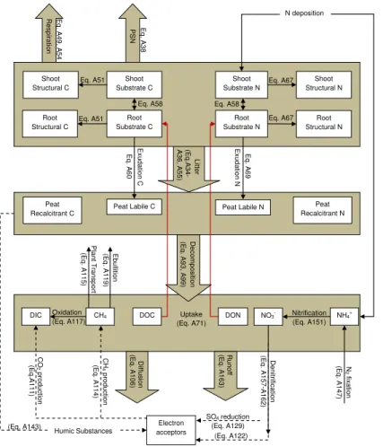
Differences in the mobility of C and N compartments were implemented using a two-pool concept throughout the model. Similar to decomposition models that distinguish the quality of soil organic matter (Grant et al., 1993; Parton et al., 1993), C and N are presented in labile (L) and recalcitrant (R) pools in SOM. In addition, the model
5
differentiates C and N pools based on quality in vegetation, into structural (struc) pools (Fig. 2). The pasture vegetation model HMP (Thornley et al., 1995; Thornley, 1998b) was adopted, where C and N in grass and legumes were separated in structural and substrate pools in shoots (sh) and roots (rt) for 4 age categories. Considering our focus on competition between plant functional types, vegetation was not conceptualized in
10
term of age categories but instead classified into 3 plant functional types (PFTs) (j: 1=
mosses, 2=graminoids and 3=shrubs) that are characterized by distinctive ecological functions (Fig. 3) in our model. The composition of plants, as a result of net primary production and litter fall, is adjusted to physical conditions and N input and alters SOM quality via changes in litter quality (Q).
15
2.2 Structural adaptations for modeling peatland biogeochemistry
Modifications were made to the adopted algorithms of the MMWH and HPM models for compatibility with our modeling purpose and model structure. The main modifications and novel features of the PEATBOG model are:
2.2.1 Competition among Plant Functional Types (PFTs)
20
Plant functional types compete for light and nutrients through their morphology and nutrient utilization. We modified the algorithms of competition among plant functional
types for these controls to better represent the shading effects among PFTs and
the nutrient poor environment. Competition among plants was modeled using PFTs previously, where the depth and biomass of roots mainly determined superiority in
GMDD
6, 1599–1688, 2013PEATBOG
Y. Wu and C. Blodau
Title Page
Abstract Introduction
Conclusions References
Tables Figures
◭ ◮
◭ ◮
Back Close
Full Screen / Esc
Printer-friendly Version
Interactive Discussion
Discussion
P
a
per
|
Dis
cussion
P
a
per
|
Discussion
P
a
per
|
Discussio
n
P
a
per
|
competition (Van Oene et al., 1999; Pastor et al., 2002; Heijmans et al., 2008). We focused instead on the effect of light for PFT competition that is controlled by shading effects through canopy layers (Fig. 3). This differs from the utilization of the leaf area index, which determines the share of total photosynthesis in the HMP model (Thornely et al., 1995). In the PEATBOG model, the uptake of N is also modified to be specific for
5
each soil layer and PFT. It includes the uptake of three forms of N in the PFTs so that N availability varies for roots of each PFT in the same location. In addition to inorganic N sources (NH+4 and NO−3), as modeled in some C and N cycling models (Aber et al., 1997; Van der Peijl and Verhoeven, 1999), DON is included as a third N source, ac-knowledging its abundance (Moore et al., 2005a) and potential importance in nutrient
10
poor environments, such as bogs (Jones et al., 2005; Nasholm et al., 2009) (Fig. 3).
2.2.2 Decoupling of O2boundary and WT boundary
The interface between oxic and anoxic conditions and unsaturated and saturated peat (i.e. the water table position, WT) are separately modeled and control biogeochemical and physical processes, respectively. Recent findings questioned that the long-term
15
WT is the sole control on biogeochemical processes in peat as well as the acrotelm
andcatotelmconcept in modeling of peatlands (Morris et al., 2011). Meanwhile O2was found well above and below the WT in peats, for instance during drying and rewetting experiments in a degraded fen site with dense soil (Estop-Aragon ´es et al., 2012). The decoupling of redox conditions from the WT spatially and temporally in dense soils
20
is potentially important for the partitioning of respired C into CO2 and CH4 during the decomposition of peat. We calculated O2concentration in each layer to regulate energy limited processes such as CH4 oxidation and peat decomposition. Water table, on the other hand, serves as a control on moisture limited biological or physical processes, such as root metabolism and diffusion.
GMDD
6, 1599–1688, 2013PEATBOG
Y. Wu and C. Blodau
Title Page
Abstract Introduction
Conclusions References
Tables Figures
◭ ◮
◭ ◮
Back Close
Full Screen / Esc
Printer-friendly Version
Interactive Discussion
Discussion
P
a
per
|
Dis
cussion
P
a
per
|
Discussion
P
a
per
|
Discussio
n
P
a
per
|
2.3 Submodel 1 – environmental controls
Physical boundary conditions, such as day length, degree days, water table depth, soil moisture, temperature and depth profiles of O2, are generated by the model to control physicochemical and biological processes.
Day length (DL), which in the model controls photosynthesis, varies for geographic
5
position of the site and day of year. The daily day length value is obtained from the angel between the setting sun and the south point, which in turn is calculated from the declination of the earth and the geographical position of the site (Brock, 1981) (Appendix A, Eq. A14, A15). Declination of the earth is the angular distance at solar noon between the sun and the equator and positive for the Northern Hemisphere. The
10
value of declination is approximately calculated by Cooper (1969) using the day of the year.
Temperature is modeled by sinusoidal equations (Carslaw and Jaeger, 1959) and modified by converting a dampening depth into thermal conductivity (Appendix A, Eq. A13). Thermal conductivity (Kthermal) is adjusted for each layer for peat
com-15
paction and snow coverage that delays the thermal exchange in winter and early spring (Fig. S1a in the Supplement).
Degree-days (DD) represent the accumulation of cold days and trigger defoliation (Frolking et al., 2002; Zhang, 2002). Similar to other models, defoliation occurs on the day when DD reaches minus 25 degrees, with accumulated temperature of lower than
20
0 degrees after day 181 of the year (1 July in non-leap years).
Water table (WT) depth is simulated by calculating the water table depth from the water storage of peat using a modified version of the Mixed Water and Heat model (MMWH) (Granberg et al., 1999). Precipitation and snow melt represent water in-puts, and are obtained from local meteorological records, instead of modeling the
25
GMDD
6, 1599–1688, 2013PEATBOG
Y. Wu and C. Blodau
Title Page
Abstract Introduction
Conclusions References
Tables Figures
◭ ◮
◭ ◮
Back Close
Full Screen / Esc
Printer-friendly Version
Interactive Discussion
Discussion
P
a
per
|
Dis
cussion
P
a
per
|
Discussion
P
a
per
|
Discussio
n
P
a
per
|
per unit of the peatland surface is calculated from a base EPT rate and multipliers of plant leaf area (Reimer, 2001) (Appendix A, Eq. A3), daily air temperature (Fig. S1b), daily average photosynthetic active radiation (PAR), and a factor of WTD and rooting depth (Lafleur et al., 2005a) (Fig. S2c). A maximum water storage was added to allow overflow once the WT rises above the peat surface. WTD is then obtained from linear
5
functions of water storage as in the MMWH model but with depth-dependent slopes (Appendix A, Eq. A8). The WT layer is defined as the layer in which the WT is located. Depth profiles of soil moisture (m3water m−3pore space) are generated by the Van Genuchten’s soil water retention equation, parameterized by Letts et al. (2000) for peat-lands (Appendix A, Eq. A9). Porosity is a function of depth derived from field
measure-10
ments for the Mer Bleue Bog (Blodau and Moore, 2002).
In order to simulate exports of dissolved C and N without modeling water movement explicitly, runoffwas distributed over 20 layers and divided into horizontal and vertical flows (Fig. 4, Appendix A, Eqs. A4–A7). The vertical advection rate depends on slope and is determined as a fraction of the total runoff. It is consistently applied to all layers.
15
The remaining runoffis horizontally distributed among layers according to the vertical hydraulic conductivity distribution. In the Mer Bleue Bog, saturated hydraulic conduc-tivity rapidly declines with depth in the acrotelm, ranging from 10−7 to 10−3m s−1 and reaches 10−8 to 10−6m s−1 in the catotelm (Fraser et al., 2001). In layers above the WT, the actual hydraulic conductivity is lower when pores are unsaturated (Hemond
20
and Fechner-Levy, 2000) (Fig. S1d).
The depth profiles of O2concentrations are simulated to locate the oxic-anoxic inter-face. Oxygen diffuses from the surface to deeper soil layers and is consumed directly or indirectly by the oxidization of peat C to CO2(Appendix A, Eq. A12). For the simulation of oxygen-dependent biogeochemical processes we chose a dichotomous distribution
25
GMDD
6, 1599–1688, 2013PEATBOG
Y. Wu and C. Blodau
Title Page
Abstract Introduction
Conclusions References
Tables Figures
◭ ◮
◭ ◮
Back Close
Full Screen / Esc
Printer-friendly Version
Interactive Discussion
Discussion
P
a
per
|
Dis
cussion
P
a
per
|
Discussion
P
a
per
|
Discussio
n
P
a
per
|
2.4 Submodel 2 – vegetation
Carbon in vascular plants is represented by four pools: shoot substrate C (sh subsC), root substrate C (rt subsC), shoot structural C (sh strucC), and root substrate C (rt subsC) (Fig. 2). Substrate C and structural C refer to metabolic activated C and recalcitrant C, respectively. Substrate pools conduct metabolic activities (i.e.
photo-5
synthesis, respiration) and structural pools perform phenological activities (i.e. growth, litter production). The flow from substrate C to structural C leads to plant growth (Ap-pendix A, Eq. A33). Each C pool or flow is bound to a N pool or flow by the C/N ratio of the specific pool. Furthermore, shoots are divided into stems and leaves and roots into coarse and fine roots by ratios specific to the PFT. Mosses are represented by 4
above-10
ground pools and two compartments:capitulum and stem. The C and N contained in
exudates are transferred from the vegetation into the uppermost labile C and N pools in the soil. Unlike N uptake by vascular plants from soil water, N uptake by mosses is restricted to atmospheric supply.
Most C and N material flows are driven by C concentration gradients except for a few
15
processes controlled by N (i.e. N uptake, N recycling from litter production). The phe-nology and competing strategies of PFTs are modeled as follows: (1) considering the seasonal C and N loss in leaves of deciduous shrubs; (2) PFT-specific N flows dur-ing growth, recycldur-ing and litter production; (3) competition among PFT is implemented through shading effects, tolerance to moisture and temperature, distribution of C and
20
N among shoots and roots, as well as turnover rates. In general, the photosynthetic nutrient-use efficiency (the ratio of photosynthesis rate and nitrogen content per leaf area) is higher in herbaceous than in evergreen woody species (Hikosaka, 2004). The growth rates in deciduous species (graminoids and deciduous shrubs) are higher than in evergreen shrubs, which in turn is higher than in mosses (Chapin III and Shaver,
25
GMDD
6, 1599–1688, 2013PEATBOG
Y. Wu and C. Blodau
Title Page
Abstract Introduction
Conclusions References
Tables Figures
◭ ◮
◭ ◮
Back Close
Full Screen / Esc
Printer-friendly Version
Interactive Discussion
Discussion
P
a
per
|
Dis
cussion
P
a
per
|
Discussion
P
a
per
|
Discussio
n
P
a
per
|
2.4.1 Photosynthesis (PSN) and competition for light
Competition for PAR is implemented through shading effects. The light level that reaches a specific PFT after interception by a taller PFT determines the C assimila-tion of this PFT (Fig. 3). For each PFT, canopy PSN is integrated from daily leaf PSN by a light attenuation coefficient (kext), leaf area index (LAI) and day length (DL)
(Ap-5
pendix A, Eq. A38). The coefficientkext is unitless, the values are 0.5 for graminoids (Heijmans et al., 2008), 0.97 for shrubs (Aubin et al., 2000), and assumed to be 0.9 for mosses. LAI is determined by leaf structural C mass and specific leaf area (SLA) of the PFT. The PSN rate for the top canopy layer of each PFT (LeafPSNj) is calculated by a non-rectangular hyperbola (Fig. S2f, Appendix A, Eq. A40). The two parameters
10
αj andξcontrol the shape of the hyperbola curves. Parameterαj represents the pho-tosynthetic efficiency, which is controlled by WT depth, the air temperature (Tair) and atmospheric CO2 level (CO2,air) (Appendix A, Eq. A42). The spring PSN of mosses starts when the snow depth falls below 0.2 cm. The variable LIj is the PAR incepted by the canopy of PFTj (umol m−2s−1). The assumptions here were that radiation
dimin-15
ishes along with canopy depth and each canopy depth contains one PFT solely. The asymptote of leaf photosynthesis rate (Pmax in g CO2m−2s−1) is regulated by
Tair, CO2,air, WT depth, N content in plant shoots and the season. The maximum PSN rate (Pmax,20, g CO2m−2s−1) occurs in an optimal environment, is also referred to as PSN capacity, and is often derived from measurements. The values of Pmax,20
20
vary among and within growth forms and follow the general sequence of decidu-ous>evergreens>mosses (Chapin III and Shaver, 1989; Ellsworth et al., 2004). The maximum PSN ratePmax,20 is 0.002 g CO2m−2s−1 for graminoids and mosses follow-ing HPM (Thornley, 1998a), and 0.005 g CO2m−2s−1for shrubs based on the ranges in Small (1972). The temperature dependences (fT,Pmax,j) ofPmaxis conceptualized as
sig-25
GMDD
6, 1599–1688, 2013PEATBOG
Y. Wu and C. Blodau
Title Page
Abstract Introduction
Conclusions References
Tables Figures
◭ ◮
◭ ◮
Back Close
Full Screen / Esc
Printer-friendly Version
Interactive Discussion
Discussion
P
a
per
|
Dis
cussion
P
a
per
|
Discussion
P
a
per
|
Discussio
n
P
a
per
|
with PFT-specific base (aw,j) for vascular plants (Fig. S2a, b). The model considers season and nutrient availability effects on Pmax. Seasonal change (fseason,Pmax) affects mosses alone between 0 to 1 and was derived from the maximum rates of carboxyla-tion (Vmax) in spring summer and autumn (Williams and Flanagan, 1998) (Fig. S2c).
Potential N stress on photosynthesis is modeled by using PFT-specific
photosyn-5
thetic N use efficiencies. Although there are interacting controls on the N economy of plant photosynthesis, such as N effects on Rubisco activity, Rubisco regeneration and the distribution of N in leaves, there seems to be a generalized linear relation of fo-liar N content and PSN capacity across growth forms and seasons (Sage and Pearcy, 1987; Reich et al., 1995; Yasumura et al., 2006). The ratio of PSN capacity and
fo-10
liar N concentration is defined as photosynthetic nitrogen use efficiency (PNUE) (Field and Mooney, 1986). In general, evergreens have lower PNUE and larger interception than the deciduous shrubs (Fig. S2d, Appendix A, Eq. A47) (Hikosaka, 2004). To re-flect N use strategies of growth forms, we implemented PNUE values for PFTs follow-ing the sequence: graminoids>shrubs>mosses, and interception values reversely. In
15
addition, a toxic effect (fN,toxic) is applied with regard to mosses when the substrate N concentration exceeds the maximum N concentration at 20 mg g−1 (Granath et al., 2009).
2.4.2 Competition for nutrients
PFTs compete for N through two processes: filtration of deposited N by mosses and
20
the uptake of N among vascular plants roots. Nitrogen deposited from the atmosphere is first absorbed by moss and then enters soil water to become available to vascular plants. The N/P ratio of mosses is used as a regulator of N pathways and an indicator of N saturation in mosses. A fraction of 95 % of the deposited N is absorbed by moss until the N/P ratio reaches 15 (Aerts et al., 1992), above which N absorption decreases
25
GMDD
6, 1599–1688, 2013PEATBOG
Y. Wu and C. Blodau
Title Page
Abstract Introduction
Conclusions References
Tables Figures
◭ ◮
◭ ◮
Back Close
Full Screen / Esc
Printer-friendly Version
Interactive Discussion
Discussion
P
a
per
|
Dis
cussion
P
a
per
|
Discussion
P
a
per
|
Discussio
n
P
a
per
|
uptake fraction declines to zero. Due to the lack of P pools in the current model version, the initial moss N/P ratio is assumed to be 10 in mosses (Jauhiainen et al., 1998).
The competition for uptake of N among PFTs is conducted through the competi-tive advantages in the architecture of the roots and capabilities for uptake of three N sources (NH−4, NO−3 and DON) (Fig. 3).The root distribution in soil is modeled using
5
an asymptotic equation (Gale and Grigal, 1987; Jackson et al., 1996) with a PFT-specific distribution coefficient (rt k) (Murphy et al., 2009) (Appendix A, Eq. A27). Graminoids have a larger rt k than shrubs, indicating more roots in deeper layers that allow utilization of N in deeper peat. The N uptake rate is affected by the surface area rather than the biomass of the fine roots. Specific root lengths LVj that vary with root
10
diameters are used to convert the dry biomass to the surface area of roots (Kirk and Kronzucker, 2005). The diameters of the fine roots were set to be between 0.005 to 0.1 cm for the “true fine roots” that are responsible for N uptake (Valenzuela-Estrada et al., 2008).
Nitrogen uptake is modeled using Michaelis–Menten equations (Appendix A,
15
Eqs. A71–A73), controlled by the soil temperature, the root biomass of the layer
and the substrate C and N concentrations in plants. Parameters Vmax and Km for
the DIN uptake were derived from the model of Kirk and Kronzucker (2005) while those for DON uptake were calibrated based on one of the few quantitative
stud-ies for an Arctic Tundra (Kielland, 1994), where Vmax for DON uptake was 0.0288
20
to 0.048 mmol g−1day−1 for shrubs (Ledum) and 0.012 to 0.096 mmol g−1day−1 for graminoids (Carex/Eriophorum).The effects of substrate C and N concentration in plants on N uptake rates were derived from the HMP model (Thornley and Cannell, 1992). The half saturation constant of substrate N was adjusted to be smaller for shrubs and mosses than for graminoids. The temperature influence on N uptake is modeled
25
usingQ10 functions for active NO−3 uptake and linear functions for passive NH +
GMDD
6, 1599–1688, 2013PEATBOG
Y. Wu and C. Blodau
Title Page
Abstract Introduction
Conclusions References
Tables Figures
◭ ◮
◭ ◮
Back Close
Full Screen / Esc
Printer-friendly Version
Interactive Discussion
Discussion
P
a
per
|
Dis
cussion
P
a
per
|
Discussion
P
a
per
|
Discussio
n
P
a
per
|
of DON uptake by plants is limited to low molecular weight DON (e.g. glycine, aspar-tate and glutamate) (Jones et al., 2005). We assumed a fraction of 0.2 of total DON concentration to be bio-available to plants, according to reports on arctic tundra and two permafrost taiga forests (Jones and Kielland, 2002; Atkin, 2006). Pools of NH+4, NO−3, and DON are simulated in thedissolved C and N submodel.
5
2.5 Submodel 3 – soil organic matter dynamics
Thesoil organic matter (SOM)submodel simulates peat decomposition and accumula-tion using a multi-layer approach. The litter produced from thevegetationsubmodel is added to the topsoil layer and into the rooted layers of the peat. In each layer, C and N is present in labile (L) and recalcitrant (R) pools. The decomposition of eachSOMpool
10
was modeled following the single pool model of Manzoni et al. (2010). Pool L and R are decomposed simultaneously at rates that are determined by their C/N ratios, an envi-ronmentally controlled decomposition rate constant k, and the availability of mineral N. Three fates of the decomposition products are possible: (1) leaching as dissolved organic matter (DOM), (2) re-immobilization into microbial biomass, and (3) conversion
15
into dissolved inorganic carbon (DIC) and dissolved inorganic nitrogen (DIN). DOM was extracted from SOM pools by a constant fraction, which is empirically related to the lo-cal precipitation level of the site (Appendix A, Eqs. A90, A96). The value used here (0.05) is slightly smaller than the lower end (0.06) of the suggested range for ecosys-tems in general (Manzoni et al., 2010), owing to the small hydraulic conductivity in
20
northern peatlands. The remaining SOM is either mineralized into dissolved inorganic matter or immobilized into microbial biomass with a microbial efficiency (e), indicating
the immobilized fraction of the decomposed SOM (Appendix A, Eq. A84). Parametere
is empirically calculated from the initial C/N ratios of the SOM pools, which in turn is controlled by the composition of litter produced from each PFT. For simplicity, microbial
25
GMDD
6, 1599–1688, 2013PEATBOG
Y. Wu and C. Blodau
Title Page
Abstract Introduction
Conclusions References
Tables Figures
◭ ◮
◭ ◮
Back Close
Full Screen / Esc
Printer-friendly Version
Interactive Discussion
Discussion
P
a
per
|
Dis
cussion
P
a
per
|
Discussion
P
a
per
|
Discussio
n
P
a
per
|
and negative rates indicate net immobilization. The “critical N level” is used as an indi-cator of the N concentration at which immobilization balances mineralization (Berg and Staaf, 1981). The “critical N level” varies according to the C/N ratio of microorganisms, the DOM leaching fraction,eand another factor representing the N preferences of mi-croorganisms during decomposition (αENprefer) (Appendix A, Eq. A86). The nitrogen
5
preference of microorganisms (αENprefer) is a multiplier larger than 1 and is limited by the asymptotic C/N ratio of SOM at decomposition equilibrium (Appendix A, Eq. A95). In addition to the control of N concentration in SOM, the availability of soil mineral N also affects the decomposition rates. Nitrogen addition experiments showed neutral or negative effects on the decomposition rates of SOM due to contrary effects on the
10
decomposition of labile and recalcitrant OM: a decrease in the decomposition rates of more recalcitrant OM and an increase in that of more labile OM (Neff et al., 2002; Janssens et al., 2010; Currey et al., 2011). We adopted the quantitative relation from the Integrated Biosphere Simulator model (IBIS) (Liu et al., 2005), by converting min-eral N contents to DIN concentrations in each layer (Fig. S3d). Nitrogen minmin-eralization
15
is inhibited while N immobilization is promoted by increasing DIN concentration up to 200 µmol L−1. The decomposition rate constantsk are regulated by substrate quality (q), soil moisture (f mdec), soil temperature (f Tdec) and inhibition factors accounting for the decrease in Gibbs free energy due to the accumulation of end products (i.e. CO2, CH4) in the saturated soils (Appendix A, Eq. A87). The decrease ink with depth
20
is modeled based on the “peat inactivation concept” (Blodau et al., 2011) rather than only linked to anoxia (Frolking et al., 2002) or redox potential (Zhang, 2002), as in other models. The essential idea of this concept is that the transport rate of decomposition products controls the decomposition rate in the saturated anoxic soils (Fig. S3) The inhibitions factors are values between 0 and 1 based on CO2and CH4concentrations
25
according to the inverse modeling results in Blodau et al. (2011) (Fig. S3a, b).
GMDD
6, 1599–1688, 2013PEATBOG
Y. Wu and C. Blodau
Title Page
Abstract Introduction
Conclusions References
Tables Figures
◭ ◮
◭ ◮
Back Close
Full Screen / Esc
Printer-friendly Version
Interactive Discussion
Discussion
P
a
per
|
Dis
cussion
P
a
per
|
Discussion
P
a
per
|
Discussio
n
P
a
per
|
from the long-term simulations in the spin-up runs. The moisture and temperature effect on the decomposition is each pool is modeled similar to the PCARS model (Frolking et al., 2002), with theQ10 value of the decomposition of L pools (2.3) smaller than of that of R pools (3.3) (Conant et al., 2008, 2010).
2.6 Submodel 4 – dissolved C and N
5
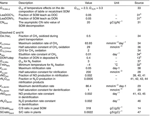
The model contains 3 dissolved C pools: CH4, CO2and DOC and 4 dissolved N pools: NH+4, NO−3, NO−2 and DON in each belowground layer (Fig. 2). Because decomposition proceeds and is controlled through the SOM pools, DOM is considered to be an end product, and is only removed by runoff. The production of DOC, DIC, DON and NH+4 are inputs from theSOM and the vegetationsubmodels. The production of DIC is further
10
partitioned into the production of CH4and CO2in the anoxic layers.
The partitioning of respired C into CO2and CH4in the saturated layers depends on the presence of alternative electron acceptors (i.e. SO2−4 , NO3 and likely humic sub-stances) for the terminal electron accepting processes (TEAP) (Conrad, 1999; Lovley and Coates, 2000). In previous studies, the ratio of CO2/CH4 production and the
pro-15
duction rates of CH4 was modeled as a function of WT depth (Potter, 1997; Zhuang, 2004), or by microbial activities using Michaelis–Menten kinetics (Segers and Kengen, 1998; Lopes et al., 2011). Following the concept put forward by Blodau (2011), we modeled the CH4production rate by an energy limited Michaelis–Menten kinetics.
We build an equation group based on the valance balance of the overall
oxidation-20
reduction process and the mass balance of C (Appendix A, Eq. A121). The first equa-tion (Appendix A, Eq. A121) denotes that CO2and CH4are the only inorganic C prod-ucts (DIC) from the decomposition of SOM. The second equation was deducted from the valance balance of CO2(+4) production and CH4(−4) production from organic C, assuming an initial oxidation state of zero as found in carbohydrates. The production of
25
GMDD
6, 1599–1688, 2013PEATBOG
Y. Wu and C. Blodau
Title Page
Abstract Introduction
Conclusions References
Tables Figures
◭ ◮
◭ ◮
Back Close
Full Screen / Esc
Printer-friendly Version
Interactive Discussion
Discussion
P
a
per
|
Dis
cussion
P
a
per
|
Discussion
P
a
per
|
Discussio
n
P
a
per
|
(CO2proEA,i) in units of electron equivalents. The acronym EA represents electron ac-ceptors other than CO2, including NO3, SO2−4 , and humic substances (HS).
In anaerobic systems, electron acceptors are consumed by terminal electron accept-ing processes that competitively consume H2or acetate. Individual processes predomi-nate according to their respective Gibbs free energy gain, usually in the sequence NO3,
5
Fe (III), humic substances (HS), SO2−4 and CO2 (Conrad, 1999; Blodau, 2011). Owing to the extremely fast turnover of H2 pools in peat, the Michaelis–Menten approach is not suitable for modeling CH4production in models running on a daily time step when H2 is considered the substrate. To avoid modeling the pools of H2and acetate explic-itly, the current model with daily time step focuses on the electron flow from complex
10
organic matter to all TEAPs, instead of modeling each microbial process explicitly. In ombrotrophic systems like bogs, only SO2−4 , NO3and HS are considered relevant elec-tron acceptors. The CO2production from SO2−4 and NO3reduction are calculated from the valance relations (Appendix A, Eq. A122). One mole of SO2−4 being reduced to HS provides 8 mole of electrons (S(+6)→S(−2)) and 1 mol of NO3releases 5, 4 and 3 mol
15
of electrons when being reduced to NO, N2O or N2(N(+5)→N(+3)→N(+1)→N(0)). Humic substances have recently also been identified as electron acceptors (Lovley et al., 1996; Heitmann et al., 2007; Keller et al., 2009) and require some considera-tion. Reduction of humic substances may be a significant CO2source in anoxic peat, where a large fraction of the total CO2 production typically cannot be explained by
20
consumption of known electron acceptors (Vile et al., 2003b). Although peat stores a large amount of organic carbon as humics, likely only a small fraction of it is redox active (Roden et al., 2010). The redox-active moieties in humics have been identified as quinones, here called DOM-Q (Scott et al., 1998). Electron accepting rate con-stants of HS in sediments were reported to be 0.34 h−1and 0.68 h−1based on two
ox-25
GMDD
6, 1599–1688, 2013PEATBOG
Y. Wu and C. Blodau
Title Page
Abstract Introduction
Conclusions References
Tables Figures
◭ ◮
◭ ◮
Back Close
Full Screen / Esc
Printer-friendly Version
Interactive Discussion
Discussion
P
a
per
|
Dis
cussion
P
a
per
|
Discussion
P
a
per
|
Discussio
n
P
a
per
|
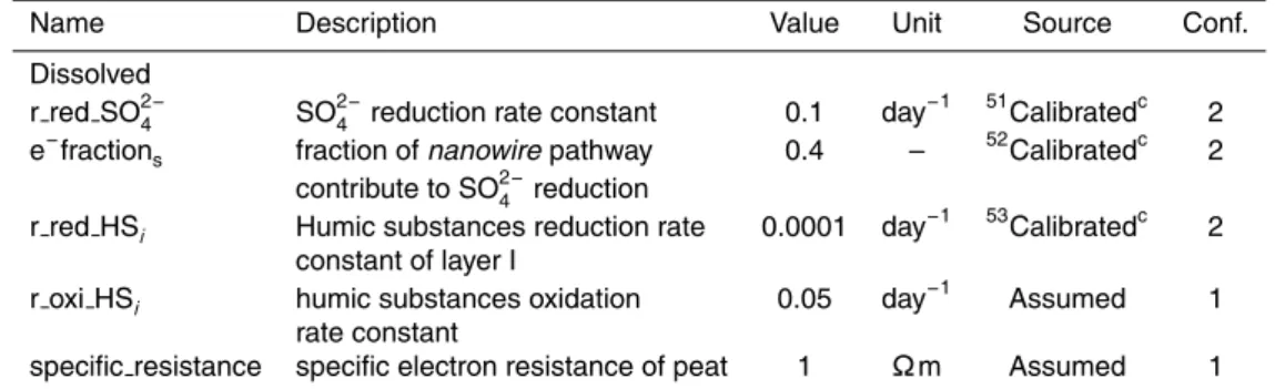
Based on this limited information, we conceptually modeled the reduction and ox-idation of humic substances using first order kinetics (Appendix A, Eq. A133–A136). The initial values of the EA (electron acceptor) and ED (electron donor) pools in the humic substances are calculated from the SOM C pool by a ratio of 1.2 eq. (mol C)−1 (Roden et al., 2010). The initial electron accepting capacity used in the model was ca.
5
2000–4000 mmol charge m−2 for the upper 60 cm of peat per m2, which is close to the capacity of 2725 mmol charge m−2derived from a drying and rewetting experiments in a minerotrophic fen (Knorr and Blodau, 2009).
In the model electron acceptors are renewed via two mechanisms: direct oxidation by O2 due to WT fluctuation in the only temporarily saturated layers and microbially
10
mediated electric currents through the peat column via an extracellular electron trans-fer (Inanowire). While the first mechanism is well documented (Knorr and Blodau, 2009), the second is speculative. It relates to the observation that even in deeper peats, that are not affected by influx of oxygen or other inorganic electron acceptors, CO2seems to be net released in excess of methane (Beer and Blodau 2007). This finding has
15
remained enigmatic because excess CO2release would be impossible from a stoichio-metric point of view when organic matter with oxidation state close to zero is respired and other, more reduced decomposition products, in particular molecular hydrogen, are not concurrently released. A relevant accumulation of molecular hydrogen has, to our knowledge, not been observed in affected peats. Anaerobic methane oxidation may
20
appear as a way out of the dilemma; however, also this process would depend on the elusive electron acceptor (Smemo and Yavitt, 2011).
Recently an extracellular electron transfer was described that has the potential to solve this enigma. Microorganisms in soils and sediments were first detected extra-cellularly utilizing electrons from redox active species, such as HS, Fe (III) (Lovley and
25
GMDD
6, 1599–1688, 2013PEATBOG
Y. Wu and C. Blodau
Title Page
Abstract Introduction
Conclusions References
Tables Figures
◭ ◮
◭ ◮
Back Close
Full Screen / Esc
Printer-friendly Version
Interactive Discussion
Discussion
P
a
per
|
Dis
cussion
P
a
per
|
Discussion
P
a
per
|
Discussio
n
P
a
per
|
“nanowires” so that oxidation and reduction process are spatially separated from each other. In our case the oxidation process releasing CO2would proceed deeper into the peat, whereas the reduction reaction would take place near the peatland surface where oxygen is present. We suppose that this mechanism may be the reason for some of the frequently observed CO2production that is unrelated to physical supply of an electron
5
acceptor deeper into the peat. Not knowing about mechanistic detail in peats, we con-ceptualized this process by simply calculating an extracellular electron current in the peat and using Ohm’s law for the anoxic layers (Appendix A, Eq. A137). Peat electron flow resistance (R) is determined by inverse modeling based on the resistance constant definition and corrected for soil moisture under the assumption that air filled pore space
10
cannot conduct electrons (Appendix A, Eq. A142). The parameter ρpeat (Ωm) is the specific resistance of the material andl is the layer depth (m). Electron current in mA was then converted to mmol by the Avogadro constant (NA) and the Faraday constant (F) (96490 C mol−1) (Appendix A, Eq. A137). To make this process work, electrochem-ical potential gradients (dEh) that drive the flow between adjacent layers are needed.
15
In absence of meaningful measurements of redox potential of peat we calculated such a gradient from a measured redox potential gradient in the Mer Bleue Bog that was given by concentration depth profiles of dissolved H2, CO2, and CH4. We assumed that the redox potential gradient of this redox couple represents the minimum depth gradient in electrochemical potentials being present. Using the Nernst equation for the
20
reaction 4H2(aq)+CO2(aq)→2H2O(l)+CH4(aq) (Appendix A, Eq. A138–A141), con-centration profiles were converted into electrochemical potential gradients with depth.
H2 concentration was measured by Beer and Blodau for the Mer Bleue bog (2007)
(Table S4).
In the model the electron flow through the peat towards the peatland surface is used
25
GMDD
6, 1599–1688, 2013PEATBOG
Y. Wu and C. Blodau
Title Page
Abstract Introduction
Conclusions References
Tables Figures
◭ ◮
◭ ◮
Back Close
Full Screen / Esc
Printer-friendly Version
Interactive Discussion
Discussion
P
a
per
|
Dis
cussion
P
a
per
|
Discussion
P
a
per
|
Discussio
n
P
a
per
|
based on the S deposition on the site at 0.89 mmol S m−3day−1 (Vile, 2003a). The same thermodynamic inhibition concept as used to model methanogenesis was ap-plied also to bacterial sulfate reduction (Appendix A, Eq. A129).
Both CO2and CH4are in equilibrium between gaseous phase and dissolved phase
obeying Henry’s Law (Appendix A, Eq. A100–A103). The efflux of C and N are through
5
runoffand advection in dissolved phase and in gaseous phase from the soil surface. Diffusion follows Fick’s law with moisture corrected coefficients in the saturated layers and was modeled as step functions in the unsaturated layers where diffusion acceler-ates by orders of magnitude for gases (Appendix A, Eq. A104–A107). CH4also escape from the soil via ebullition and plant mediated transportation (Appendix A, Eq. A115–
10
A120). Ebullition occurs in saturated layers once CH4level exceeds the maximum con-centration CH4,max. The parameter CH4,max is sensitive to temperature and pressure (Davie et al., 2004), with a base maximum CH4 concentration at 500 uM, which is the value for a vegetated site at 10◦C in Walter et al. (2001). The ebullition of CH4 re-leases the gas to the atmosphere without it passing through the unsaturated zone.
15
In the rooted layers, graminoids transport CH4 at rates that are determined by the biomass of the graminoid roots. A percentage of 50 % of the CH4are oxidized to CO2 during the plant mediated transportation by the O2in plant tissues (Walter et al., 2001). The CH4 oxidation in the oxic layers was modeled using temperature sensitive double Michaelis–Menten functions (Segers and Leffelaar, 2001) (Appendix A, Eq. A118).
20
The gases N2O and NO are byproducts of nitrification and denitrification (NH+4 →
NO−2 →NO−3 →NO2−→NO→N2O→N2) in the anoxic layers. During nitrification, the fraction of N loss as NO (rNOnitri) is 0.1 %–4 % day−1 with a mean value of 2 % (Baumg ¨artner and Conrad, 1992; Parsons et al., 1996). For N2O (rN2Onitri) this value is smaller at 0.1 %–0.2 % day−1(Ingwersen et al., 1999; Breuer et al., 2002; Khalil et al.,
25
GMDD
6, 1599–1688, 2013PEATBOG
Y. Wu and C. Blodau
Title Page
Abstract Introduction
Conclusions References
Tables Figures
◭ ◮
◭ ◮
Back Close
Full Screen / Esc
Printer-friendly Version
Interactive Discussion
Discussion
P
a
per
|
Dis
cussion
P
a
per
|
Discussion
P
a
per
|
Discussio
n
P
a
per
|
1984; Riedo et al., 1998). In an acidic environment, nitrification was detected to cease below pH of 4 and reached a maximum at a pH of 6 (L ˚ang et al., 1993). The optimal range of pH for denitrification was suggested to be from 6 to 8 (Heinen, 2006). Tem-perature factors were empirically modeled, using the equation in DNDC (Li and Aber, 2000) for nitrification and the common formalism equation in NEMIS (Johnsson et al.,
5
1987; H ´enault and Germon, 2008) for denitrification.
3 Model application
3.1 Site description
The model was applied on the Mer Bleue (MB) Bog for a period of 6 yr from 1999 to 2004 to evaluate the simulation performances WT dynamics, carbon fluxes, soil water
10
DIC and CH4concentrations and C and N budgets against observations.
The Mer Bleue Bog (45◦51′N; 75◦48′W) is a raised acidic ombrotrophic bog of 28 km2located 10 km east of Ottawa, Ontario. The bog was formed 8400 yr ago as a fen and developed into a bog between 7100 and 6800 yr BP. The peat depth varies from 5 to 6 m at the center to<0.3 m at the margin (Roulet et al., 2007). The vegetation
cover-15
age is dominated by mosses (e.g.Sphagnum capillifolium, S. angustifolium, S. magel-lanicum and Polytrichum strictum) and evergreen shrubs (e.g. Ledum groenlandicum, Chamaedaphne calyculata). Some deciduous shrubs(Vaccinium myrtilloides), sedges (Eriphorum Vaginatum), black spruce (Picea marinana) and larch also appear in some areas (Moore et al., 2002). The annual mean air temperature record from the local
20
GMDD
6, 1599–1688, 2013PEATBOG
Y. Wu and C. Blodau
Title Page
Abstract Introduction
Conclusions References
Tables Figures
◭ ◮
◭ ◮
Back Close
Full Screen / Esc
Printer-friendly Version
Interactive Discussion
Discussion
P
a
per
|
Dis
cussion
P
a
per
|
Discussion
P
a
per
|
Discussio
n
P
a
per
|
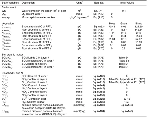
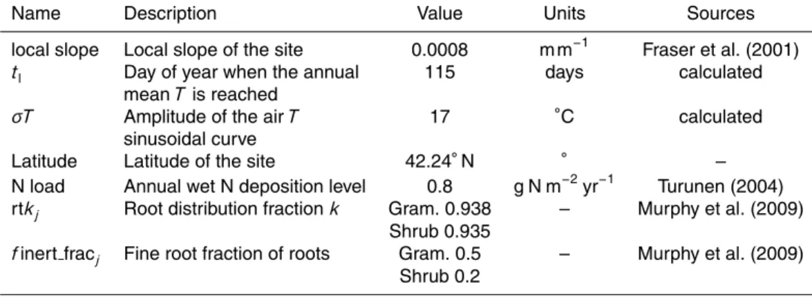
3.2 Application data and initialization
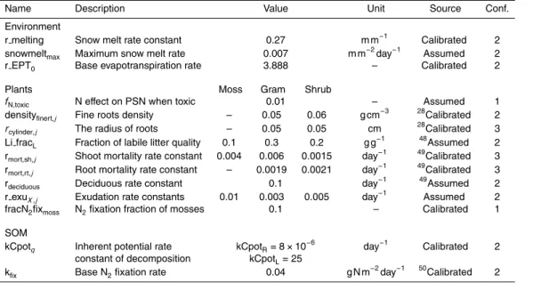
Inputs required are geographic location and local slope of the site, daily precipitation and PAR, daily snow depth record, annual average and range of air temperature, at-mospheric CO2, CH4 and O2 levels, annual N load and vegetation type of the site (Table 2).
5
Observed C fluxes, water table depth, and the depth profiles of temperature and moisture with 5 s to 30 min intervals were obtained fromFluxnet Canada(http://fluxnet. ccrp.ec.gc.ca) and averaged to daily values. Fluxes were determined using microme-teorological techniques and short gaps were filled by linear interpolation between the nearest measured data points. Other data sets for model evaluation were obtained
10
from a range of the published literature. The spin-up (initiation) of the model was con-ducted with initial values obtained from literature (Table S4) and the meteorological and geophysical boundary conditions (Table 2) from 1999 to 2004 obtained from Fluxnet Canada. The time series was repeated every 6 yr until the model approached its steady state after a period of longer than 100 yr. The obtained values of state variables were
15
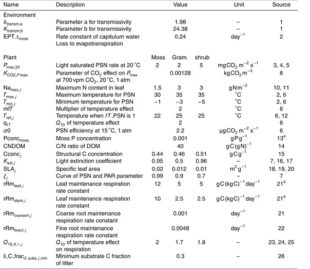
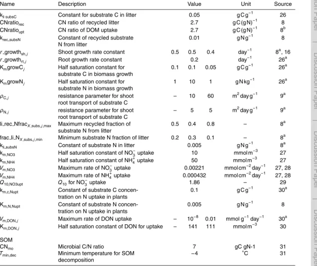
used for the actual model application and evaluation. Most parameters were obtained from literature for bogs or peatlands in general, or calibrated for the ranges from mea-surements, or in line with the values used in previously published models. In total, 29 out of 140 parameters were calibrated and ranked from 3 to 1 based on their origin and descending confidence in their accuracy and correctness (Tables 3 and 4).
Parame-20
GMDD
6, 1599–1688, 2013PEATBOG
Y. Wu and C. Blodau
Title Page
Abstract Introduction
Conclusions References
Tables Figures
◭ ◮
◭ ◮
Back Close
Full Screen / Esc
Printer-friendly Version
Interactive Discussion
Discussion
P
a
per
|
Dis
cussion
P
a
per
|
Discussion
P
a
per
|
Discussio
n
P
a
per
|
4 Results
We ran the parameterized, initiated model for 6 yr from 1999 to 2004 and evaluated the simulation results of WT depth, and depth profiles of soil temperature, moisture and O2 to assess the ability of the model to generate environmental controls on C and N cy-cling. The simulated C and N pool sizes, transfer rates and fluxes were compared with
5
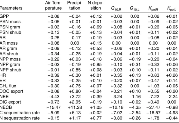
six years of continuous measurements to evaluate the capability of the model in quan-tifying C and N pools and cycling rates. We also conducted sensitivity analysis for the key factors (e.g. temperature, precipitation, N deposition) and a range of uncertain cal-ibrated parameters (e.g. potential decomposition rate of the soil organic matter). This demonstrated the sensitivity of the model to N availability and climate controls, which
10
shows the potential for applying the model to long- term N fertilization and N deposi-tion and climate change studies. As statistics for evaluadeposi-tion we chose the root mean square error (RMSE), linear regression coefficient (r2), and the index of agreement (d) (Willmott, 1982).
4.1 WT depth, soil temperature and moisture
15
Simulated daily average soil temperature was plotted against measured temperatures in hummocks at 0.05 m and 0.8 m depth (Fig. 5a). The simulations agreed well with
the observations and showed degrees of agreement (d) of 0.97 and 0.95, and RMSE
of 3.23 and 1.70 degrees, respectively. However, the model failed to simulate the ob-served deviation from the sinusoidal temperature curve when snow was not present
20
in the winter of 2003, implying other controls on soil temperature that are currently missing in the model.
In general, the simulated WT depth showed good agreement with the observed data, with a degree of agreement (d) of 0.98 and RMSE of 0.06 m (Fig. 5b). The largest devi-ation was from mid-July to early August of 1999, when the simulated WT depth for some
25
GMDD
6, 1599–1688, 2013PEATBOG
Y. Wu and C. Blodau
Title Page
Abstract Introduction
Conclusions References
Tables Figures
◭ ◮
◭ ◮
Back Close
Full Screen / Esc
Printer-friendly Version
Interactive Discussion
Discussion
P
a
per
|
Dis
cussion
P
a
per
|
Discussion
P
a
per
|
Discussio
n
P
a
per
|
changes from summer to fall when the deviations of more than 10 cm occurred for 10 to 30 days. These disparities were likely owed to the simple bucket model structure that lacks processes of water transfer that buffer variations in water content.
Considering the large variation of soil moisture between hummocks and hollows, we compared the simulation at 0.2 m and 0.4 m depth with the observations in hummock
5
and hollows, respectively (Fig. 5c). The seasonal dynamics were well captured and the 0.4 m simulation agrees with the observation strongly. However, the simulated volumet-ric water content at 0.2 m was systematically overestimated by 0.1 to 0.2 in summers and up to 0.5 for the wettest year in winter. Large spatial in situ variability of observed volumetric water content might be one of the reasons for this large discrepancy, as the
10
simulated values are similar to other measurements in hummocks in the Mer Bleue Bog during even drier years (Wendel et al., 2011).
4.2 Daily carbon fluxes
Gross ecosystem production (GEP) was calculated as the sum of simulated gross pri-mary production (GPP) of all PFTs (Fig. 6a). The simulated ecosystem respiration
15
(ER) was the release of CO2 gas from the peat surface, which included autotrophic respiration (AR) in shoots and roots of plants and the heterotrophic respiration (HR) of microorganisms in the soil (Fig. 6b). Net ecosystem exchange (NEE) was calculated as the difference between ER and GPP (Fig. 6c).
Overall, the simulated GPP, ER and NEE captured the seasonal dynamics and the
20
magnitudes of the C fluxes. The maximum simulated daily GPP was 5.96 g C m−2day−1 and occurred in the driest year 1999, which is similar to the maximum observed 6.80 g C m−2day−1. The simulated starting dates of spring PSN ranged from day 79 (2000) to day 99 (2001), with an average date of day 90. These values fell in the re-ported range from day 86 to day 101 (Moore et al., 2006). The simulated starting dates
25
GMDD
6, 1599–1688, 2013PEATBOG
Y. Wu and C. Blodau
Title Page
Abstract Introduction
Conclusions References
Tables Figures
◭ ◮
◭ ◮
Back Close
Full Screen / Esc
Printer-friendly Version
Interactive Discussion
Discussion
P
a
per
|
Dis
cussion
P
a
per
|
Discussion
P
a
per
|
Discussio
n
P
a
per
|
(±0.42 g CO2m−2day−1) in measurements (Moore et al., 2006). Statistic analysis re-vealed a root mean square error (RMSE) of 0.73 g C m−2day−1and a degree of agree-ment (d) of 0.95 (Fig. 7a). However, there were a few days when the simulation errors
were large, among which the maximum underestimation was 3.68 g C m−2day−1 on
31 July in 2000 and the maximum overestimation was 3.21 g C m−2day−1 on 23 May
5
2002.
ER simulation followed a seasonal trend with winter values being smaller than 1 g C m−2day−1and summer peaks of 5 to 7 g C m−2day−1. The summer peaks were higher than the field estimates from 2.07 to 4.67 g C m−2day−1, the latter was how-ever likely to be underestimated by 20 % on average considering the measuring and
10
calculation methods (Lafleur, 2003). The average difference between simulation and
observation was 0.43 g C m−2day−1, which was small compared to the calculated
error of GPP (±0.42 g C m−2day−1) and to the potential correction factor of NEE (1.21±0.12 g C m−2day−1) (Lafleur, 2003; Moore et al., 2006). Overall, ER was over-estimated in dry summers, i.e. in 1999, 2001, 2002 and 2003, with a maximum
dis-15
crepancy of 4.18 g C m−2day−1in the driest and hottest summer in 2003 (Fig. 6b). The
maximum underestimates of ER was 2.81 g C m−2day−1 in 22 July 2004, during the
period when the WT was underestimated most. The daily simulation has a degree of agreement of 0.92 and RMSE 0.64 g C m−2day−1(Fig. 7a).
NEE was calculated from the simulated ER and GPP fluxes, therefore the absolute
20
errors were enlarged in the simulation of NEE (Fig. 6c). The simulated peak uptake of NEE appeared annually during summer; during spring the bog took up carbon and in fall and winter lost it, as documented by measurements (Lafleur, 2003). The maximum simulated uptake occurred during the same period as in the observations, from June to early July, with values <−2.5 g C m−2day−1 while the maximum loss appears mostly
25