Thiago Antonini Alves
[email protected] Universidade Tecnológica Federal do Paraná Engenharia Mecânica 84016-210 Ponta Grossa, PR, Brasil
Carlos A. C. Altemani
[email protected] Universidade Estadual de Campinas Faculdade de Engenharia Mecânica Departamento de Energia 13083-970 Campinas, SP, Brazil
Conjugate Cooling of a Discrete
Heater in Laminar Channel Flow
Electronic components are usually assembled on printed circuit boards cooled by forced airflow. When the spacing between the boards is small, there is no room to employ a heat sink on critical components. Under these conditions, the components’ thermal control may depend on the conductive path from the heater to the board in addition to the direct convective heat transfer to the airflow. The conjugate forced convection-conduction heat transfer from a two-dimensional strip heater flush mounted to a finite thickness wall of a parallel plates channel cooled by a laminar airflow was investigated numerically. A uniform heat flux was generated along the strip heater surface. Under steady state conditions, a fraction of the heat generation was transferred by direct convection to the airflow in the channel and the remaining fraction was transferred by conduction to the channel wall. The lower surface of the channel wall was adiabatic, so that the heat conducted from the heater to the plate eventually returned to the airflow. A portion of it returned upstream of the heater, preheating the airflow before it reached the heater surface. Due to this, it was convenient to treat the direct convection from the heater surface to the airflow by the adiabatic heat transfer coefficient. The flow was developed from the channel entrance, with constant properties. The conjugate problem was solved numerically within a single solution domain comprising both the airflow region and the solid wall of the channel. The results were obtained for the channel flow Reynolds number ranging from about 600 to 1900, corresponding to average airflow velocities from 0.5 m/s to 1.5 m/s. The effects of the solid wall to air thermal conductivities ratio were investigated in the range from 10 to 80, typical of circuit board materials. The wall thickness influence was verified from 1 mm to 5 mm. The results indicated that within these ranges, the conductive substrate wall provided a substantial enhancement of the heat transfer from the heater, accomplished by an increase of its average adiabatic surface temperature.
Keywords: conjugate heat transfer, adiabatic heat transfer coefficient, laminar channel flow, numerical analysis
Introduction1
The purpose of the present work was to perform an analysis of the conjugate forced convection-conduction heat transfer from a small 2D foil heater flush mounted to the lower plate (substrate) of a horizontal channel, as indicated in Fig. 1. The substrate thickness (t) and its thermal conductivity (ks) were known and a laminar developed airflow was forced into the channel. The lower surface and both ends of the substrate plate were adiabatic, so that only the upper face, in contact with the airflow, could exchange heat by forced convection. There were two thermal paths available for heat transfer from the heater to the airflow. One was by convection, directly from the heater upper surface to the airflow. The other was from the heater lower surface by conduction and spreading in the substrate wall. The heat transfer through this path was transferred back to the airflow by convection at the upper substrate surface, both upstream and downstream of the heater. This substrate conduction presents two opposing effects to the heater cooling by the airflow. First, a thermal boundary layer development upstream the heater reduces the direct convective heat transfer from the heater to the airflow. On the other hand, the effective heat transfer area to the airflow increases due to the conductive spreading upstream and downstream the heater. If this effect prevails over the first one, there will be a heat transfer enhancement, as compared to the case of an adiabatic substrate plate.
The effects of the laminar airflow rate, the fluid to substrate thermal conductivities ratio and the substrate thickness were considered in the present analysis. The total heat dissipation rate in the heater was assumed known, but its distribution into the direct convection to the airflow and the conduction to the substrate wall was obtained from analysis. The convective heat transfer was characterized by the adiabatic heat transfer coefficient had, due to its independence on the thermal boundary conditions (Moffat, 1998; Alves and Altemani, 2008). The heat transfer coefficient based on the inlet flow temperature (Tin) was also evaluated for comparison
Paper received 2 February 2011. Paper accepted 23May 2011. Technical Editor: Horácio Vielmo.
with the adiabatic coefficient. This problem depends also on the heater length and position in the channel. In the present work, the heater length was equal to the channel height and its upstream edge was centered on the substrate.
whenever a Biot number based on the ratio of the module’s resistance to conduction over that to convection was greater than 1. Sugavanam et al. (1995) presented a numerical analysis of the conjugate heat transfer from 2D uniformly powered strip heaters flush mounted on the lower wall of a horizontal parallel plates channel. The substrate wall upper surface was cooled by laminar forced convection and the lower surface was either adiabatic or subject to laminar forced convection. The dependence of the heat transfer from the heat source was investigated for a wide range of parameters, including the substrate to coolant fluid thermal conductivities ratio (ks/k), the heat source position and the channel Reynolds number. The results indicated that preheating of the flow by board conduction increased with the ratio (ks/k), decreasing the Nusselt number on the heat source. The reference temperature for the Nusselt number was the fluid inlet temperature. It was verified that the effects of substrate thickness were important only for the conductivity ratio (ks/k) > 10. The average Nusselt on the heater surface decreased with an increase in (ks/k) for fully developed flow, due solely to substrate conduction effects. This decrease was more pronounced for smaller values of the Reynolds number, due to the relative increase of the substrate conduction effect. Considering a uniform flow at the channel entrance, developing along the channel length, the average Nusselt on the heater surface decreased as the source moved to downstream positions in the channel. Cole (1997) presented an analysis for the conjugate convective-conductive heat transfer from a 2D strip heater flush mounted on the surface of a conductive plate of finite thickness. The plate was cooled on the heater side by a fluid flow with a linear velocity profile, while the opposite surface was adiabatic. The reference temperature for the Nusselt number was that of the coolant fluid far from the plate surface, typical for external flows. The heat transfer numerical results were presented in terms of a conjugate Peclet number. It was found that for large values of this parameter, the heat transfer is dominated by the fluid flow and the strip heater size is the appropriate length scale. For small values, the appropriate scale was the solid thickness. Wang and Jaluria (2004) considered the effects of the three-dimensional conjugate mixed convection and conduction heat transfer from two heaters flush mounted on the lower wall of a horizontal rectangular duct. The two heaters were deployed with both streamwise and spanwise separation on the wall. The effects of the wall to fluid thermal conductivities ratio and the Reynolds number in the laminar regime, considering a single value of the Grashoff number, were presented in the numerical results. Among their conclusions, the heaters spanwise distribution may result in lower average temperature for the two sources. Considering a duct with an aspect ratio of 10, they reported that the numerical results of temperature distribution on the solid-fluid interface were slightly lower than those of Sugavanam et al. (1995). This was attributed to conduction in the spanwise direction, associated to the three-dimensional simulations.
In the present investigation, a numerical solution of the conjugate problem was performed for a single domain comprising both the solid and fluid regions. The reference temperature selected to describe convective heat transfer from the heater was its average adiabatic surface temperature. Thus, the corresponding average adiabatic heat transfer coefficient is independent of the amount of airflow preheating upstream of the heater. This preheating is due to the thermal wake generated by conduction upstream of the heater through the substrate plate.
Natural convection effects were considered negligible in the present work, a procedure adopted in similar investigations (e.g., Alves and Altemani, 2010; Zeng and Vafai, 2009; Davalath and Bayazitoglu, 1987 and Ramadhyani et al., 1985). In order to present a perspective for this consideration, reference will be made to the work of Kang et al. (1990). They performed experiments to
investigate the mixed convection from a single heat source module mounted on a thin horizontal plate well insulated at the back surface. Their results indicated that the heat transfer from the module is dominated by forced convection when (Gr/Re5/2) < 0.9.
The Reynolds number Re was based on the heater length and the forced flow average velocity. The Grashoff number was Gr = gβq"(L+2H)L3/(kυ2), where L and H indicate respectively the heater length and height, and q" is the convective heat flux from the module to the fluid. When the heater is flush mounted on the substrate plate, the height is H = 0. For any specified value of Re, their correlation gives the upper limit of Gr for which natural convection effects may be neglected.
The results of the present investigation are important for the thermal design of electronic components assembled on circuit boards cooled by forced convection. The conjugate forced convection and conduction heat transfer must be accounted for, and this analysis is most important under conditions of limited available spacing between the boards. In this case, heat sinks may not be allowed for cooling purposes and the heat transfer enhancement due to heat spreading along the substrate wall may be an important contribution to the total heat transfer (Alves, 2010).
Nomenclature
cp = specific heat, J/(kg.K)
g* = influence coefficient
h = convective heat transfer coefficient, W/(m2.K)
H = channel height, m
k = air thermal conductivity, W/(m.K)
ks = substrate thermal conductivity, W/(m.K)
L = total channel length, m
Ld = downstream length, m
Lh = heater length, m
Lu = upstream length, m
m& = mass flow rate, kg/s Nu = Nusselt number Pe = Peclet number Pr = Prandtl number
q = convective heat transfer rate per unit heater depth,W/m q" = heat flux, W/m2
Re = Reynolds number, Eq. (2)
t = substrate thickness, m
T = temperature, K
u = velocity component along the plates, m/s
U = dimensionless u – velocity component, Eq. (6)
x, y = Cartesian coordinates, m
X, Y = dimensionless Cartesian coordinates, Eq. (6)
Greek Symbols
ρ = density, kg/m3
µ = dynamic viscosity, Pa.s
θ = dimensionless temperature, Eq. (6)
ξ = dimensionless coordinates
Subscripts
ad = adiabatic
d = downstream
f = fluid
h = heater
in = inlet
m = mixed mean
s = substrate
u = upstream
Superscripts
Analysis
Problem formulation and heat transfer parameters
A small foil heater (length Lh) is flush mounted on a conductive substrate with thickness t and thermal conductivity ks in a horizontal channel of length L and height H, as indicated in Fig. 1. The substrate lower and side surfaces, as well as the channel upper surface, are all adiabatic.
Figure 1. Schematic of the conjugate heat transfer problem.
A laminar airflow, with constant properties evaluated at 300 K, was developed from the channel entrance, with uniform velocity u and the analytical parabolic velocity profile given by
( )
(
2)
2 4 1 2 3 H y u y
u = − ,
2 2
H y
H≤ ≤
− (1)
The average airflow velocity u and the channel hydraulic diameter defined the Reynolds number
µ
ρu H
Re= 2
(2)
The heater upstream edge was positioned at Lu = L/2 on the upper substrate surface. A heat dissipation rate equal to qh per unit depth normal to Fig. 1 was uniformly distributed along the heater length, with a heat flux qh′′= qh/Lh . This heat flux was distributed either directly to the airflow above the heater, with local flux qf′′(x),
or to the substrate under the heater, with a local flux qs′′(x). Under steady state conditions, a local energy balance along the heater requires that
( )
x q( )
x qqh′′= f′′ + s′′
(3)
The local heat fluxes qf′′(x) and qs′′(x) were obtained by an iterative numerical solution of the energy equation in the conjugate domain indicated in Fig. 1, comprising the solid substrate, the heater and the flow regions. In dimensionless form, the energy conservation equations respectively for the solid and fluid regions were expressed as follows:
(
22 22)
1
0, s
k
Pr k X Y
θ θ
∂ +∂ =
∂ ∂ 0≤ ≤X 1,
(
2)
2H t H
Y
L L L
− + ≤ ≤ − (4)
(
22 22)
1
,
U
X Pr X Y
θ ∂θ ∂θ
∂ = +
∂ ∂ ∂ 0≤ ≤X 1, 2 2
H H
Y
L L
− ≤ ≤ (5)
The dimensionless variables were
L x
X= ,
L y
Y= ,
µ ρuL
U= ,
(
)
h h in L q T T k ′′ − =
θ (6)
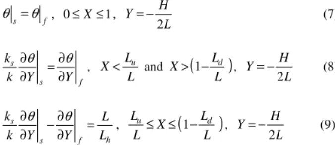
Equations (4) and (5) were solved simultaneously, subject to the following boundary conditions. The upper and lower surfaces of the domain, as well as the upstream and downstream ends of the substrate plate were adiabatic. At the channel inlet, the fluid temperature was uniform at Tin, which corresponds to θin = 0. The outflow boundary was treated with negligible diffusion. At the substrate-fluid interface, the temperature and heat flux continuity were imposed as follows.
s f
θ =θ , 0≤X≤1,
L H Y 2 − = (7) f s s Y Y k k ∂ ∂ = ∂ ∂θ θ
,
L L X< u
and
(
)
L L X> − d
1 , L H Y 2 − = (8) h f s s L L Y Y k k = ∂ ∂ − ∂ ∂θ θ
,
(
)
L L X L
Lu≤ ≤ 1− d
, L H Y 2 − = (9)
Equation (9) is the dimensionless form of the local energy balance expressed by Eq. (3). The heater surface temperature Th(x) and the heat fluxes qf′′(x) and qs′′(x) were not uniform along the heater length Lh. They were integrated along the heater length to obtain, respectively, the average heater temperature and the heat transfer rates qf from the heater directly to the airflow and qs to the solid substrate.
( )
∫
= h L h hh T x dx
L
T 1 , =
∫
′′( )
h
L f
f q xdx
q , =
∫
′′( )
h
L s
s q xdx
q
(10)
Obviously, the local energy balance expressed by Eq. (3), after integration over the heater length, results in the overall energy balance qh = qf + qs.
Two average convective heat transfer coefficients were defined
on the heater surface. One was had, based on the heater average
adiabatic surface temperature, Tad. This coefficient is important because it is independent of the thermal conditions upstream the heater (Alves and Altemani, 2008). The heater adiabatic surface temperature may be obtained mostly, simply considering an adiabatic substrate wall, because in this case it is equal to the airflow inlet temperature. In this case, all dissipated heat is transferred directly to the airflow (qf = qh), so that
)
(
s 0h ad
h h in k
q h
L T T =
=
− (11)
The average adiabatic Nusselt number over the heater was expressed by
0 1 s ad h ad h k h L Nu
k θ =
= = (12)
The other average heat transfer coefficient was hin, based on the uniform inlet flow temperature Tin. It was obtained considering a conductive substrate (ks≠ 0), for which a fraction (qf /qh) of the total dissipation rate qh was transferred directly to the airflow, defined by:
Lu Lh Ld
)
(
fin
h h in
q h
L T T
=
− (13)
The corresponding average Nusselt number in this case was
1 f in h in
h h
q h L Nu
k q θ
= =
(14)
For a conductive substrate, the heater average temperature rise above the inlet flow temperature (Th– Tin ) is due to two effects. The direct convective heat transfer rate qf from the heater to the airflow is responsible for the heater temperature rise above its adiabatic temperature, (Th–Tad). The heat transfer rate qu conducted through the substrate wall upstream the heater returns by convection to the airflow. This effect gives rise to a thermal wake responsible for the heater adiabatic temperature rise above the inlet flow temperature, (Tad– Tin). These two effects may be added as follows:
(
Th−Tin) (
= Th−Tad) (
+ Tad−Tin)
(15)Due to imperfect fluid mixing in the channel, the adiabatic temperature rise (Tad– Tin) is always greater than the corresponding fluid mixed mean temperature rise (Tm,u – Tin). The ratio of these two temperature differences defined a coefficient gu∗. An energy balance in the flow region upstream the heater related (Tm,u – Tin) to
qu and the airflow rate m& .
(
)
(
)
uad in m.u in u u
p
q
T T T T g g
m c
∗ ∗
− = − =
ɺ (16)
Similarly, the heater average temperature rise (Th–Tad) was
related, by an influence coefficient g∗h, to the corresponding fluid mixed mean temperature rise (∆Tm)h, which was expressed in terms of qf and the flow rate m& .
(
−)
=( )
∗= ∗h p f h h m ad
h g
c m
q g T T T
&
∆ (17)
Substituting Eqs. (16) and (17) into Eq. (15),
(
−)
= ∗+ ∗u p u h p f in
h g
c m
q g c m
q T T
&
& (18)
Defining the Peclet number Pe = RePr, Eq. (18) was obtained in dimensionless form.
(
∗+ ∗)
= u
h u h h f
h g
q q g q q Pe
2 θ
(19)
The fractions (qf /qh) and (qu /qh) and the upstream coefficient g∗u depend on the conduction through the substrate and were obtained for each test condition. The convective coefficient g∗h, on the other hand, depends solely on the flow conditions and it was obtained from numerical tests considering an adiabatic substrate wall.
Problem formulation and heat transfer parameters
The energy equations (4) and (5) were solved simultaneously within the conjugate domain indicated in Fig. 1, comprising the solid substrate and the flow regions, using the control volumes method (Patankar, 1980). The convection and diffusion in the flow region, described by Eq. (5), with fully developed flow in the channel, were treated by the power-law scheme. The linear system of algebraic equations obtained from the discretization process was solved iteratively using the line-by-line TDMA method. The numerical results were obtained imposing the stated boundary conditions and the temperature and heat flux continuity expressed by Eqs. (7) to (9) along the substrate-fluid interface. Equations (7) and (8) were automatically satisfied by the use of the harmonic mean for evaluation of the diffusion coefficients at the control volumes interfaces. Equation (9) indicates the distribution of the uniform heat flux qh′′ into the local heat fluxes qf′′(x) and qs′′(x) and required an iterative solution procedure, described as follows. Along the heater length, the link between the adjacent solid and fluid control volumes, respectively below and above the heater, was removed. An initial guess of the heat fluxes qf′′(x) and qs′′(x) was assumed and used to apply source terms to the referred solid and fluid control volumes. Then, the energy equations (4) and (5) were solved and the numerically obtained temperature distributions, together with Eq. (9), were used to evaluate a new heater temperature distribution Th (x) on the solid substrate-fluid interface. In the present work, a perfect thermal contact was assumed between the heater and the substrate. From the evaluated Th (x), new distributions for qf′′(x) and qs′′(x) were obtained and the process was repeated until convergence. Then, the upstream heating rate qu was obtained from the substrate temperature distribution and Eq. (19) was employed to determine the coefficientgu∗.
The results were obtained with a non-uniform two-dimensional numerical grid deployed on the solution domain, comprising 300 control volumes in the flow direction and 24 to 40 control volumes in the transversal direction. In the flow direction, the grid was most refined over the heater, which contained 80 uniformly distributed control volumes. Along the upstream length Lu, 170 control volumes were uniformly deployed, and 50 others were distributed along the downstream length Ld. Along the y-direction, the grid consisted of 20 non-uniform control volumes along the height H and 4 control volumes uniformly distributed along each mm of the substrate thickness t. In the flow region, the grid size was finer near the upper and lower solid surfaces and increased with a geometric progression toward the center of the channel.
80 points along the heater and a non-uniform grid with only 20 points in the y-direction, the average Nusselt number was within 0.05% of the value previously obtained by extrapolation. When a conductive substrate was considered, additional tests verified that 4 grid points per mm along the y-direction in the solid region were enough to obtain results independent of further grid refinement. The grid used to obtain the results for a substrate thickness t /H = 0.5 is presented in Fig. 2. It is non-uniform and contains 300 control volumes along the flow and 40 control volumes in the transversal direction.
Figure 2. Non-uniform grid for t /H = 0.5, with (300 x 40) control volumes.
The iterative solution process was interrupted when the absolute changes of the heater average temperature θh, the average Nusselt
number Nuin, and the heat flow ratio (qs/qh) between two consecutive iterations were smaller than 10-5. The numerical results
were obtained in a microcomputer (Intel® Pentium® D processor 2.8 GHz and 1GB RAM), in about 10 minutes for a typical solution considering a conductive substrate.
Results
The numerical results were obtained considering a channel length L = 0.2 m and the plates spacing H = 0.01 m. The heater length was Lh = 0.01 m, with its upstream edge at Lu = 0.1 m from the channel entrance. Five values were considered for the substrate thickness t, from 1 to 5mm. The effect of the substrate conductivity was investigated for five values of (ks/k) in the range from 10 to 80. The flow was always in the laminar regime and five values of the Reynolds number were considered, in the range from about 600 to 1900 (average air velocities from 0.5 m/s to 1.5 m/s). The air properties were obtained from tabulated values at 300 K (Incropera et al., 2006).
Shah and London (1978) presented a laminar flow correlation for the local Nusselt number along a parallel plates channel with uniform heat flux on the walls, defined as follows.
( )
( )
( )
( )
k H T Tq Nu
m h
2 ξ ξ
ξ ξ
− ′′ =
(20)
It is based on a dimensionless coordinate ξ with origin at the heater upstream length, ξ = (x – Lu) / (2H RePr), on the local mixed mean airflow temperature Tm (ξ) and on the channel hydraulic diameter. Their correlation is given by
( )
1 31 490 /
Nu ξ = . ξ− , ξ≤0 0002. (21)
( )
1 31 490 / 0 4
Nu ξ = . ξ− − . , 0 0002. ≤ ≤ξ 0 001. (22)
This correlation can be associated with that along the heater on the adiabatic substrate in the present work. A local Nusselt number
Nuad (ξ) based on the adiabatic heater temperature (which is equal to
Tin when ks = 0), and on the heater length, can be related to that defined in Eq. (20) by
( )
( )[ ( )
( )
( )
]
h m h
in h ad
L H T T
T T Nu
Nu 2
ξ ξ
ξ ξ ξ
− −
= (23)
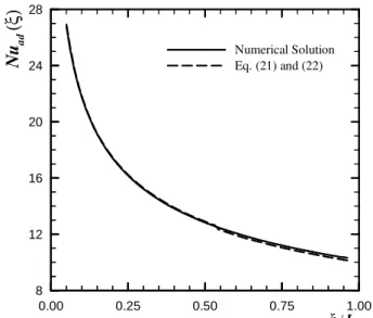
After substituting the correlation Eq. (21) or (22) on the left side of this equation, the resulting Nuad(ξ) from the right side was compared with the numerical distribution obtained in the present work for a particular value of Re. The results obtained for Re = 1890 are shown in Fig. 3. They indicated that the predictions from Eq. (21) were 0.5% above the present numerical results, while Eq. (22) predicted values 1.4% below the numerical values.
Figure 3. Comparison of the numerical results with predictions from Eqs. (21) and (22).
The influence coefficient gh∗, defined by Eq. (17), was obtained from simulations for an adiabatic substrate wall, because this is the simplest procedure. For the adiabatic substrate, Tad= Tinand all the heat is transferred directly to the airflow by convection, qf = qh . The results presented in Fig. 4 are, however, valid for either an adiabatic or a conductive substrate. They indicate that the coefficient gh∗ increases with the Reynolds number, due to larger mass flow rates. This coefficient was correlated to the Reynolds number by
0 66
0 339 .
h
g∗= . Re
(24)
The heater average adiabatic Nusselt number Nuad, as defined by Eq. (12), was obtained considering an adiabatic substrate (qf = qh and qu = 0). The heater average adiabatic temperature was obtained from Eqs. (19) and (24) and the result was replaced on the right side of Eq. (12), giving rise to the correlation
34 0 475
1 .
ad . PrRe
Nu =
(25) X
0.40 0.45 0.50 0.55 0.60 0.65
ξ /Lh
N
u
ad
(ξ
)
0.00 0.25 0.50 0.75 1.00
8 12 16 20 24 28
Figure 4. Heater influence coefficient gh.
Figure 5. Heater average adiabatic Nusselt number for air.
This Nusselt number does not depend on the thermal conditions – it changes only with the flow conditions and the results for air (Pr = 0.707) are presented in Fig. 5 as a function of the Reynolds number.
For a conductive substrate, an upstream airflow heating qu gives rise to a temperature increase (Tad– Tin). This temperature rise was
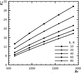
expressed with the help of the upstream coefficient gu∗ defined by Eq. (16), obtained from the simulations of the conjugate problem. Considering for example t/H = 0.5, the dependence of the coefficient gu∗ on the Reynolds number is presented in Fig. 6, for distinct values of (ks/k). It increases with the Reynolds number, mainly due to larger mass flow rates. For a given Re, this coefficient decreases as (ks/k) increases, due to larger upstream heating (qu) through the substrate wall. The dependence on Re was similar for thinner substrates, but the values of gu∗ increased due to larger conductive spreading resistances associated with thinner walls.
Table 1 presents the numerical results of g∗u for the ratio (ks/k) = 80, encompassing the five substrate thicknesses and the five Reynolds numbers considered in the present work.
Figure 6. Upstream coefficient gu for t /H = 0.5.
Table 1. Upstream coefficient gu for (ks/k) = 80.
t H Re
630 945 1260 1575 1890
0.1 11.7135 15.7673 19.4808 22.9660 26.2619
0.2 9.9132 13.3525 16.5058 19.4598 22.2690
0.3 8.9720 12.0842 14.9435 17.6347 20.1873
0.4 8.3516 11.2594 13.9273 16.4329 18.8213
0.5 7.9088 10.6621 13.1960 15.5729 17.8417
The heat transfer fractions (qf /qh), (qs /qh) and(qu /qh) were also obtained from the simulations of the conjugate problem. The first two fractions obviously add to unity, as can be checked by integration of Eq. (3) along the heater length, with the definitions of Eq. (10). The fraction (qs/qh) is presented in Fig. 7 for the substrate thickness t/H = 0.5, indicating that most of the heat transfer occurs through the substrate plate, except for the lowest (ks/k). As expected, the ratio (qs/qh) increased with the ratio (ks/k), due to smaller conductive spreading resistance, and it decreased as Re increased, due to larger direct convective heat transfer. The results of (qs/qh) for (ks/k) = 80 are presented in Table 2, showing that for any Re it increases with the substrate thickness, due also to smaller conductive spreading resistance.
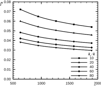
The fraction (qu/qh) conducted upstream of the heater for
t/H = 0.5 is presented in Fig. 8, considering the effects of Re and the ratio (ks/k). The effect of the substrate thickness t on (qu/qh) is presented in Table 3 for (ks/k) = 80. They follow a trend similar to (qs/qh) with respect to the effects of t, (ks/k) and Re. Comparing the data in Table 2 and Table 3, it is seen that about 60 per cent of the conduction heat transfer from the heater to the substrate wall is released to the airflow upstream of the heater.
Re
g
h500 1000 1500 2000
20 25 30 35 40 45 50 55
*
Re
N
u
ad500 1000 1500 2000
7 8 9 10 11 12 13 14 15 16
Re
g
u500 1000 1500 2000
4 8 12 16 20 24 28 32
10 20 40 60 80
ks/k
*
*
* *
Figure 7. Fraction (qs /qh) for t /H = 0.5.
Table 2. Fraction (qs /qh) for (ks /k) = 80.
t H Re
630 945 1260 1575 1890
0.1 0.6224 0.6012 0.5858 0.5737 0.5636
0.2 0.7170 0.6988 0.6854 0.6747 0.6658
0.3 0.7624 0.7460 0.7339 0.7243 0.7162
0.4 0.7899 0.7749 0.7637 0.7547 0.7472
0.5 0.8085 0.7944 0.7839 0.7754 0.7683
Figure 8. Fraction (qu /qh) for t /H = 0.5.
Table 3. Fraction (qu /qh) for (ks /k) = 80.
t H Re
630 945 1260 1575 1890
0.1 0.3804 0.3665 0.3565 0.3487 0.3422
0.2 0.4401 0.4283 0.4196 0.4128 0.4072
0.3 0.4693 0.4587 0.4509 0.4448 0.4397
0.4 0.4873 0.4774 0.4702 0.4645 0.4597
0.5 0.4993 0.4899 0.4831 0.4777 0.4732
The heater average dimensionless temperature θh was obtained from the previous results and the Peclet number (Pe), using Eq. (19). The distribution of θh for t/H = 0.5 is presented in Fig. 9, showing the expected temperature decrease as the mass flow rates increases with the Reynolds number. It also shows the heater temperature decrease as the substrate thermal conductivity increases. The results for the thermal conductivities ratio (ks/k) = 80 are presented in Table 4, showing that the heater average temperature decreases with the Reynolds number and the substrate thickness. The temperatures θh presented in Table 4 were obtained from Eq. (19) and they matched those obtained directly from the numerical simulations within 10-4.
Figure 9. Dimensionless heater average temperature for t /H = 0.5.
Table 4. Dimensionless heater average temperature for (ks /k) = 80.
t H Re
630 945 1260 1575 1890
0.1 0.0604 0.0545 0.0506 0.0478 0.0456
0.2 0.0499 0.0452 0.0421 0.0399 0.0382
0.3 0.0443 0.0403 0.0376 0.0357 0.0342
0.4 0.0408 0.0371 0.0347 0.0329 0.0316
0.5 0.0382 0.0348 0.0326 0.0310 0.0297
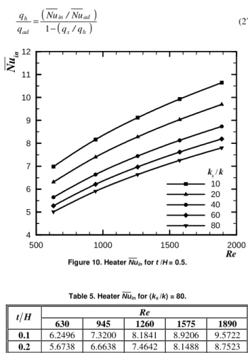
The heater average Nusselt number based on Tin depends on the ratio (ks/k) and the Reynolds number. It may be obtained either directly from the numerical simulations, or from the previous results for (qf /qh) and θh, as indicated by Eq. (14). The Nuin distribution obtained for t/H = 0.5 is presented in Fig. 10. It increases with Re
due to larger airflow rates, but decreases with (ks/k) due to a larger conductance of the substrate wall. As the substrate thickness t
decreases, larger conductive wall resistances increase Nuin, as indicated by the numerical results presented in Table 5 for the case with (ks/k) = 80.
Compared to the adiabatic substrate, the conductive substrate provides additionally a conductive path for heat transfer from the heater. Considering the same inlet flow and heater average temperatures and flow rate in the channel, the conductive substrate causes an enhancement of heat transfer from the heater when compared to the adiabatic substrate. It was evaluated as follows. An adiabatic substrate transfers heat to the airflow only by convection, at a rate qad. For a conductive substrate, the direct convective heat
Re
q
s/
q
h500 1000 1500 2000
0.10 0.20 0.30 0.40 0.50 0.60 0.70 0.80 0.90
10 20 40 60 80
ks/k
Re
q
u/
q
h500 1000 1500 2000
0.05 0.10 0.15 0.20 0.25 0.30 0.35 0.40 0.45 0.50 0.55
10 20 40 60 80
ks/k
Re
θ
h500 1000 1500 2000
0.00 0.01 0.02 0.03 0.04 0.05 0.06 0.07 0.08
10 20 40 60 80
transfer from the heater to the airflow is equal to qf. From the
definitions of Nu ad and Nuin, Eq. (11) and (13), the ratio of these two heat transfer rates was expressed by
(
)
ad in
ad f
Nu Nu q
q
=
(26)
When the heat transfer rate qf obtained from this equation is substituted into the heater overall energy balance, qh = (qf +qs), an expression for the heat transfer enhancement due to the conductive substrate is obtained in the form
(
)
(
s h)
ad in
ad h
q / q
Nu / Nu q
q
− =
1 (27)
Figure 10. Heater Nuin for t /H= 0.5.
Table 5. Heater Nuin for (ks /k) = 80.
t H Re
630 945 1260 1575 1890
0.1 6.2496 7.3200 8.1841 8.9206 9.5722
0.2 5.6738 6.6638 7.4642 8.1488 8.7523
0.3 5.3591 6.3070 7.0725 7.7246 8.3020
0.4 5.1548 6.0712 6.8140 7.4490 8.0081
0.5 5.0094 5.9070 6.6324 7.2541 7.8012
This result is presented in Fig. 11 for t/H = 0.5 and also in Table 6, for (ks/k) = 80. The enhancement increases with both (ks/k) and t, due to a greater conductance of the substrate wall. The effect of the Reynolds number is not obvious from Eq. (27) because, as
can be seen from the previous results, the ratio (Nuin/Nuad) increases with the Reynolds number, while the ratio (qs/qh) decreases, causing opposing trends to (qh/qad). In the present investigation, the effect of (qs /qh) was slightly dominant – the heat transfer enhancement decreased slightly with the Reynolds number. The presented results indicate a significant heat transfer enhancement due to substrate conduction – the heat transfer ratio (qh /qad) ranged from about 150% to 280%.
Due to the substrate adiabatic lower surface, the heat conducted upstream of the heater through the substrate wall eventually returns to
the airflow and causes an increase (Tad– Tin) of the heater average adiabatic temperature above the inlet flow temperature. This undesirable temperature rise was compared to the total heater average temperature rise above the inlet flow temperature, (Th– Tin). From Eqs. (16) and (18):
(
∗ ∗)
∗
+ = −
−
h u
f u
u
in h
in ad
g q q g
g T
T T T
(28)
Figure 11. Heat transfer enhancement (qh /qad) for t /H = 0.5.
Table 6. Heat transfer enhancement (qh /qad) for (ks /k) = 80.
t H Re
630 945 1260 1575 1890
0.1 1.7714 1.7113 1.6704 1.6397 1.6153
0.2 2.1457 2.0627 2.0058 1.9629 1.9286
0.3 2.4140 2.3151 2.2470 2.1955 2.1543
0.4 2.6259 2.5146 2.4378 2.3795 2.3329
0.5 2.7997 2.6786 2.5947 2.5309 2.4795
Figure 12. Ratio (Tad – Tin )/(Th – Tin ) for t /H = 0.5.
Re
N
u
in500 1000 1500 2000
4 5 6 7 8 9 10 11 12
10 20 40 60 80
ks/k
Re
q
h/
q
ad
500 1000 1500 2000
0.00 0.50 1.00 1.50 2.00 2.50 3.00
10 20 40 60 80
ks/k
Re
(
T
ad
−
T
in)/(
T
h−
T
in)
500 1000 1500 2000
0.00 0.05 0.10 0.15 0.20 0.25 0.30 0.35 0.40 0.45 0.50
10 20 40 60 80
Table 7. Ratio (Tad – Tin )/(Th – Tin ) for (ks /k) = 80.
t H Re
630 945 1260 1575 1890
0.1 0.3311 0.3175 0.3081 0.3010 0.2951
0.2 0.3928 0.3787 0.3690 0.3615 0.3554
0.3 0.4264 0.4120 0.4021 0.3947 0.3886
0.4 0.4483 0.4340 0.4239 0.4163 0.4103
0.5 0.4639 0.4493 0.4393 0.4316 0.4255
The results obtained for the ratio of these temperature differences are presented in Fig. 12 for t/H = 0.5 and in Table 7 for (ks/k) = 80, within the investigated range of the Reynolds number. They show that from 25% to 45% of the total heater average temperature rise is due to the thermal wake originating from the upstream heated floor of the conductive substrate. This ratio increases with the substrate conductivity and thickness, while it decreases slightly with the Reynolds number, as expected. It should be kept in mind, however, that the average adiabatic temperature rise is the effect of the enhanced total heat transfer from the heater. Under the same inlet flow conditions and heater average temperature, the direct convective heat transfer from the heater to the airflow is smaller for the conductive substrate than for the adiabatic substrate. This decrease is, however, more than compensated by the total heat transfer rate from the heater in the case of the conductive substrate, as it has been shown by the results presented in Fig. 11 and Table 6.
Conclusions
The conjugate forced convection and conduction heat transfer from a strip heater flush mounted to a finite thickness wall (substrate) of a parallel plates channel were investigated numerically, using the control volumes method. The investigation was performed considering laminar airflow fully developed from the channel entrance. A uniform heat flux qh′′ was released along the heater length and it was transferred to the airflow and to the conductive substrate wall. The local distribution into the direct convective heat flux qf′′(x) from the heater to the airflow and the
conductive heat flux qs′′(x) from the heater to the substrate wall were not known a priori and they were obtained by an iterative procedure. These two heat fluxes were integrated along the heater length to evaluate its convective and conductive heat losses. The convective heat loss qf was expressed by means of the adiabatic heat transfer coefficient, because it is independent of the thermal conditions. The heater average temperature θh was expressed by means of two influence coefficients: the upstream influence coefficient g∗u, and the self-heating influence coefficient g∗h. The first coefficient evaluated the heater average adiabatic temperature rise above the inlet flow temperature in the channel, and the second coefficient was used to evaluate the average heater temperature rise above its average adiabatic temperature. Considering a dissipation rate qh in the heater, the fraction (qs /qh) conducted through the substrate and the portion (qu /qh) conducted upstream of the heater were obtained numerically as functions of the channel Reynolds number, the thermal conductivities ratio (ks/k) and the substrate thickness t. The results indicated that a substantial fraction of heat transfer occurs by conduction through the substrate. The average
Nusselt numbers Nuin and Nuad were related to evaluate the heat
transfer enhancement due to a conductive substrate in comparison to an adiabatic substrate, indicating values from 150% to 280%. The heater average adiabatic temperature rise due to preheating of the airflow by substrate conduction was related to its total temperature rise above Tin in dimensionless form, indicating that it represents a substantial fraction of the total, ranging from 25% to 45% in the present investigation.
Acknowledgements
The support of CNPq (Brazilian Research Council) to the first author in the form of a Doctorate Program Scholarship is gratefully acknowledged.
References
Alves, T.A., 2010, “Conjugate Cooling of Discrete Heaters in Channels” (In Portuguese), Ph.D. Thesis, State University of Campinas, Campinas, SP, Brazil, 129 p.
Alves, T.A. and Altemani, C.A.C., 2008, “Convective Cooling of Three Discrete Heat Sources in Channel Flow”, J. Braz. Soc. Mech. Sci. & Eng., Vol. XXX, pp. 245-252.
Alves, T.A. and Altemani, C.A.C., 2010, “Thermal Design of a Protruding Heater in Laminar Channel Flow”, Proceedings of the 14th International Heat Transfer Conference, Washington, USA, pp. 691-700.
Anderson, A.M., 1994, “Decoupling Convective and Conductive Heat Transfer Using the Adiabatic Heat Transfer Coefficient”, ASME J.
Electronic Packaging, Vol. 116, pp. 310-316.
Cole, K.D., 1997, “Conjugate Heat Transfer from a Small Heated Strip”, I. J. Heat Mass Transfer, Vol. 40, pp. 2709-2719.
Davalath, J. and Bayazitoglu, Y., 1987, “Forced Convection Cooling Across Rectangular Blocks”, ASME J. Heat Transfer, Vol. 109, pp. 321-328. De Vahl Davis, G., 1983, “Natural Convection of Air in a Square Cavity: A Benchmark Numerical Solution”, I. J. Numerical Methods Fluids, Vol. 3, pp. 249-264.
Incropera, F.P., DeWitt, D.P., Bergman, T.L. and Lavine, A.S., 2006, “Fundamentals of Heat and Mass Transfer”, John Wiley & Sons, Hoboken, USA, 1024 p.
Incropera, F.P., Kerby, J.S., Moffatt, D.F. and Ramadhyani, S., 1986, “Convection Heat Transfer from Discrete Heat Sources in a Rectangular Channel”, I. J. Heat Mass Transfer, Vol. 29, pp. 1051-1057.
Kang, B.H., Jaluria, Y. and Tewari, S.S., 1990, “Mixed Convection Transport from an Isolated Heat Source Module on a Horizontal Plate”,
ASME J. Heat Transfer, Vol. 112, pp. 653-661.
Moffat, R.J., 1998, “What’s New in Convective Heat Transfer?”, I. J. Heat Fluid Flow, Vol. 19, pp. 90-101.
Nakayama, W., 1997, “Forced Convective/Conductive Conjugate Heat Transfer in Microelectronic Equipment”, Annual Review Heat Transfer, Vol. 8, pp. 1-45.
Patankar, S.V., 1980, “Numerical Heat Transfer and Fluid Flow”, Hemisphere Publishing Corporation, New York, USA, 197 p.
Ramadhyani, S., Moffat, D.F. and Incropera, F.P., 1985, “Conjugate Heat Transfer from Small Isothermal Heat Sources Embedded in a Large Substrate”, I. J. Heat Mass Transfer, Vol. 28, pp. 1945-1952.
Shah, R.K. and London, A.L., 1978, “Laminar Flow Forced Convection in Ducts”, Advances in Heat Transfer, Supplement No. 1, Academic Press, New York.
Sugavanam, R., Ortega, A. and Choi, C.Y., 1995, “A Numerical Investigation of Conjugate Heat Transfer from a Flush Heat Source on a Conductive Board in Laminar Channel Flow”, I. J. Heat Mass Transfer, Vol. 38, pp. 2969-2984.
Wang, Q. and Jaluria, Y., 2004, “Three-Dimensional Conjugate Heat Transfer in a Horizontal Channel with Discrete Heating”, ASME J. Heat Transfer, Vol. 126, pp. 642-647.