Computing Aggregate Queries in Raster Image
Databases Using Pre-Aggregated Data
Ang´
elica Garc´ıa Guti´
errez, Peter Baumann
∗Abstract— Computing multidimensional aggregates in raster image databases is a challenging task for geo-raster applications. In this paper, we exploit the tech-niques in OLAP to speed up aggregate query process-ing in raster image databases. We focus on a special case of the aggregation problem: computation of the basic aggregation functionsadd, average, count, max-imum,and minimum. Experimental evaluation shows that the application of the pre-aggregation framework and the resulting algorithms give much better perfor-mance compared to straightforward methods.
Keywords: Aggregation, Query-Processing, Raster Databases
1
Introduction
Remote sensing data has proved to be useful in describing information about the Earth’s surface and atmosphere. It is often collected by aircraft and satellites in form of images. These images are taken at regular time inter-vals and cover large areas of the globe, thus allowing a practical tracking of developments such as deforestation, desertification, environmental contamination, and natu-ral hazards. Moreover, comparisons of satellite images from different times make these phenomena easier to un-derstand. Hence, the nature of raster image data is often multidimensional: it can include 3-D image time series (x/y/t), 3-D exploration data (x/y/z), and 4-D climate models (x/y/z/t), to name few examples. Notably, the long-term availability of remote sensing data is indispens-able to many types of analysis in Geo-applications, e.g., to study water, energy, and mineral resource problems; therefore, archives of raster image data may surpass the Petabyte size.
Typically, raster image data is stored in the database by following a so calledtiling process. That is, the image is decomposed into a set of tiles that are efficiently indexed and stored in the database. This allows that only the tiles affected by a query are retrieved from disk during
∗The work of Ang´elica Garc´ıa is supported by a grant of El Con-sejo Nacional de Ciencia y Technologia (CONACYT), scholarship 175628, by the German Academic Exchange Service (DAAD) and by Jacobs University Bremen.
Jacobs University Bremen, School of Electric Engineering and Com-puter Science, College Ring 1, 28759 Bremen, Germany. Email: [email protected]
query execution. In raster image databases, aggregation is a very important statistical concept used to represent a set of items by a single value, or to classify them into groups while determining a value for each group. The most widely used aggregations are add, average, mini-mum andmaximum. Notably, performing aggregate op-erations on large volumes of multidimensional raster data pose several challenges to existing raster database tech-nology. That is, while delivering small-sized results, large data portions have to be touched during query evaluation. In application domains such as Geographic Information Systems (GIS), the computation of many fundamental operations requires the usage of aggregate functions [3] but to the best of our knowledge, pre-aggregation support has been provided for one single operation, namely, scal-ing(zooming). In a different application domain, most On-Line Analytical Processing (OLAP) systems adopt a pre-aggregationapproach for ensuring adequate response time during data analysis. Based on the observation that data structures and operations in both application do-mains share similarities, our approach for speeding up ag-gregate operations consists in taking existing knowledge of OLAP pre-aggregation as a basis for defining an intel-ligent pre-aggregation scheme in raster image databases. OLAP pre-aggregation addresses three main problems: View Selection, Query Rewriting and View Maintenance. Despite the high maturity of these technologies [4], it has never been attempted, to the best of our knowledge, to adapt them to the field of raster image databases.
In this paper, we focus on the problem of answering a query in the presence of pre-aggregated data. We present a pre-aggregation framework along with a cost model to study the effect of using pre-aggregation in the computa-tion of aggregate queries in multidimensional raster image databases.
2
Framework
Hereby we describe the general framework used in our study on computing aggregate queries in multidimen-sional raster image databases.
2.1
Aggregation
2.1.1 Aggregate Functions
The queries that we consider can contain arbitrary ag-gregation functions. An agag-gregation function is formally defined as follows.
Definition 2.1 An aggregation function maps a multiset of cell values in a dataset D to a single scalar value. We consider the aggregation functionscount which for a multiset returns the number of cells;add, andavg, which return the sum and average, respectively, of the cell values of a multiset; max, which returns the maximum value among the cells of a multiset; andmin which returns the minimum value among the cells of a multiset.
2.1.2 Aggregate Queries
An aggregate query Q is an aggregate operation whose query predicate may contain a multidimensional spatial component, namely spatial domain (sdom). We use the following notation to express a spatial domain:
sdom= [l1:h1, . . . , ld:hd] (1)
where the functionsl(low) andh(high) deliver lower and upper bound vectors respectively. We consider queries following theselect-from-where paradigm without nested statements. In our implementation, we are using ras-daman as a raster database management system that of-fers a declarative interface, rasql. rasql is an SQL-based query language for multidimensional raster databases based on Array Algebra [2].
2.2
Pre-Aggregation
The term pre-aggregation refers to the process of pre-computing and storing the results of aggregate queries for subsequent use in the same or similar requests.
Definition 2.2 The pre-aggregated relation P is a relation with schema P(pid,aggregateOperation,
subOperation, result, spatialDomain), whose tuples (pre-aggregates) consist of a set of pre-aggregated queries
p1, p2, . . . , pn.
The pid attribute of P joins the child relations
selection, andintervals. The relationselectionhas the schemaselections(pid, sel conditions), whereas the
rela-tionintervalshas the schemaintervals(pid, sdom).
2.3
Query and Pre-Aggregate Equivalence
Definition 2.3 An aggregate query Q and a pre-aggregate pi are equivalent if and only if all the following
conditions hold true.
1. The aggregate operation of the query Q is the same as the aggregate operation defined for the pre-aggregatepi.
2. The aggregate operation of the queryQand the pre-aggregate pi must be applied over the same raster
objects.
3. The same logical and boolean conditions, if any, ap-ply for both the query and the pre-aggreate.
4. In aggregate operations over a specific spatial do-main of an object, the extent of the spatial dodo-main for both the query Q and the pre-aggregate pi is
identical.
The decision of whether to use a pre-aggregate or not in answering a query is influenced by the structural char-acteristics of the query and the pre-aggregate. That is, by comparing the query tree structures between the pre-aggregate and the input query, one can determine if the pre-aggregated result contributesfully orpartially to the answer of the query. In the case of partial-matching, mul-tiple pre-aggregates could be considered for answering a query and further analysis should be carried out to de-termine which of all candidate pre-aggregates compensate the increased overhead. To this end, we distinguish the following types of pre-aggregates: inner, overlapped, and dominant.
2.3.1 Inner Pre-Aggregates (IPAS)
Definition 2.4 A set of pre-aggregates is called inner if the spatial domain ofQ contains the spatial domain (sd) of the aggregates. For simplicity, we assume the pre-aggregates do not intersect with each other.
IPAS = {p1, . . . , pn|pi.sd⊆ Q.sd, pi.sd∩pj.sd=∅}.
(2)
2.3.2 Overlapped Pre-Aggregates (OPAS)
Definition 2.5 A set of pre-aggregates is called over-lapped if there exist an intersection between the spatial domain (sd) of Qand those of the pre-aggregates.
2.3.3 Dominant Pre-Aggregates (DPAS)
Definition 2.6 A set of pre-aggregates is called domi-nant if the spatial domain (sd) of Q is contained in the spatial component of the pre-aggregates.
DPAS={p1, p2, . . . , pn| Q.sd⊆pi.sd}. (4)
Moreover, given anascendant-ordered DPAS
DPASasc ={p1, p2, . . . , pn| Q.sd⊆p1.sd ⊆. . .⊆pn.sd},
(5) theclosest dominant pre-aggregate (pcd) toQis given by
p1, i.e.,pcd=p1. Note that dominant pre-aggregates are only considered for answering queries using the aggregate functions: add, count,andaverage.
3
Cost Model
In this section, we introduce a cost model that allows to estimate the cost (in terms of execution time) of comput-ing a query considercomput-ing the presence of pre-aggregates as well as from raw data. The cost is driven by the number of disk I/Os required and memory accesses. These pa-rameters are influenced by the number of tiles that are required to answer the query as well as by the number and size of the cells in the datasets. We assume that it takes the same time to retrieve a tile from disk as it will take to retrieve any other tile.Similarly, we consider the time taken to access a given cell (pixel) on main memory to be the same as for any other cell.
3.1
Computing a Query from Raw Data
The cost of computing an aggregate query Q (or sub-partitions of pre-aggregates) from raw data, (Cr), is given
by
Cr= N tilesX
i=1
Cacc(tilei) + N cellsX
i=1
Cagg(celli) (6)
whereCacc is the cost of retrieving a tile required to
an-swerQ, andCaggis the cost of accessing and aggregating
the cells corresponding to the spatial domain of the query.
3.2
Computing a Query using Inner
Pre-aggregates
The cost of answering an aggregate query considering the use of inner pre-aggregated results is given by
CIP AS=Cf in(Q, P) +
|IP ASX|
i=1
Cacc(pi) +CSP, (7)
where Cf in is the cost of finding the pre-aggregates ∈
IP AS in the pre-aggregated relation P, Cacc is the
accumulated cost of retrieving the results of the pre-aggregates, andCSP is the cost of decomposing the query
Qinto a set of sub-partitions and aggregating each from raw data.
3.3
Computing a Query using Overlapped
Pre-aggregates
The cost of answering an aggregate query by using over-lapped pre-aggregated results is given by
COP AS=Cf in(Q, P)+
|OP ASX |
i=1
Cdec(pi)+
|S|
X
i=1
Cr(si)+CSP,
(8) where Cf in is the cost of finding the pre-aggregates ∈
OP AS in the pre-aggregated relationP,Cdec is the cost
of decomposing the spatial domain of each pre-aggregate into a set of sub-partitionsSsuch that the spatial domain of the partitioned pre-aggregate corresponds topi.sdom−
(pi.sdom∩ Q),Cris the cost of aggregating each resulting
sub-partitionsi ∈S from raw data, andCSP is the cost
of decomposing the queryQ into a set of sub-partitions and aggregating each from raw data.
3.4
Computing a Query using Inner and
Overlapped Pre-aggregates
The cost of answering an aggregate query considering the use of inner and overlapped pre-aggregated results is given by
CIOP AS=CIP AS+COP AS+CSP, (9)
where CIP AS andCOP AS are the costs of retrieving the
results of inner and overlapped pre-aggregates, respec-tively, and CSP is the cost of decomposing the queryQ
into a set of sub-partitions and aggregating each from raw data.
3.4.1 Cost of inner pre-aggregates
The cost of retrieving the results of inner pre-aggregates (CIP AS) is given by
CIP AS=Cf in(Q, P) +
|IP ASX|
i=1
Cacc(pi) (10)
where Cf in is the cost of finding the pre-aggregates ∈
IP AS in the pre-aggregated relation P, and Cacc is the
accumulated cost of retrieving the results of the pre-aggregates.
3.4.2 Cost of overlapped pre-aggregates
The cost of retrieving the results of overlapped pre-aggregates (COP AS) is given by
COP AS =Cf in(Q, P) +
|OP ASX |
i=1
Cdec(pi) +
|S|
X
i=1
where Cf in is the cost of finding the pre-aggregates
∈ OP AS in the pre-aggregated relation P, Cdec is the
cost of decomposing the spatial domain of each pre-aggregate into a set of sub-partitionsSsuch that the spa-tial domain of the partitioned pre-aggregate corresponds topi.sdom−(pi.sdom∩Q), andCris the cost of aggregating
each resulting sub-partitionsi∈S from raw data.
3.4.3 Cost of aggregating sub-partitions of the query
The cost of aggregating each sub-partition inSP is given by
CSP =Cdec(Q) +
|XSP|
i=1
Cr(si), (12)
where Cdec stands for the cost of decomposing Q into a
setSPof sub-partitions, andCris the cost of aggregating
each resulting sub-partitions∈SP from raw data. Note that Cdec is influenced by the costs of accessing the tiles
required to aggregate each of the sub-partitions, and by the cost of accessing the spatial properties of the pre-aggregates in IPAS and OPAS.
3.5
Computing a Query using a Dominant
Pre-aggregate
The cost of computing an aggregate queryQby using a dominant pre-aggregate is given by
CDP AS=CDP(Q, P) +Cagg(pcd), (13)
where CDP is the cost of finding the pre-aggregates ∈
DPAS in the pre-aggregated relation P and the cost of finding the closest dominant pre-aggregate pcd, whereas
Caggis the cost of computing the aggregate difference of
pcdcorresponding topcd.sdom− Q.sdom.
3.5.1 Cost of the closest-dominant pre-aggregate
The cost of aggregating sub-partitions of the closest dom-inant pre-aggregate,Cagg, can be calculated as follows
Cagg(pcd) =Cdec(pcd) +
|XSP|
i=1
Cr(si), (14)
where Cdec is the cost of decomposing pcd into a set SP
of sub-partitions, andCr is the cost of aggregating each
resulting sub-partition s∈SP from raw data.
4
Implementation
This section describes the application of the pre-aggregation framework in a raster-database management system, namely, rasdaman. The query processing mod-ule of rasdaman was extended with the pre-aggregation
framework, and it has been implemented as part of the optimization and evaluation phases.
The QueryComputation procedure returns either the resultR or an execution plan for a given query Q. The input of the algorithm is the query tree Qt
correspond-ing to a given aggregate query. The algorithm first ver-ifies if there is a perfect-matchingbetween the input query and the pre-aggregated queries. If it finds a per-fect matching then it returns the result retrieved from the pre-aggregated relation. Otherwisse, the algorithm searches for apartialMatchingbetween the query and the pre-aggregates allowing only to differ in the values for the spatial domain. If a partial-matching is found, then the decision of whether to answer the query from pre-aggregated results or from raw data will be driven by the plan that results with minimum cost. The algorithm makes use of the following auxiliary procedures.
• decomposeQuery(Qt) examine the nodes of the
query treeQtand generates a standardized
represen-tationSqt that can be treated via SQL statements.
• perfectMatching(Sqt) compares a standardized
representation of the query tree Sqt against
exist-ing pre-aggregates saved in a relation P. The out-put of this procedure is the corresponding key of the matched pre-aggregate, if found.
• fetchResult(key)retrieves the resultRof the pre-aggregate identified withkey.
Algorithm 1QueryComputation
Require: A query treeQtand a relationP withk
num-ber of pre-aggregated queries.
1: initializeR= 0, i= 0, f lag=f alse
2: Sqt=decomposeQuery(Qt) 3: whilei≤k ∧ !f lagdo
4: key=perf ectM atching(Sqt, pi) 5: if keythen
6: R=f etchResult(key)
7: return R;
8: end if 9: i+ +
10: end while 11: if !f lag then
12: plan=partialM atching(Sqt) 13: return plan;
14: end if
The algorithm PartialMatching identifies aggregate nodes in a query treeQtthat may be substituted by
Upon evaluating the cost of using the different candidate pre-aggregates, the algorithm returns the plan with the cheapest cost for the computation of the query.
Algorithm 2PartialMatching
Require: A standardized query treeQtwith nnumber
of nodes.
1: initializeIP AS, OP AS, DP AS={}, plan= ”raw”
2: foreach nodenofQt do 3: if aggregateOp(node[n])then 4: Q′=getSubtree(Qt, node[n]) 5: op=getOperation(Q′)
6: ro=getRasterObject(Q′)
7: sd=getSpatialDomain(Q′)
8: result=f indP reaggregate(op, ro, sd)
9: if result= Φthen
10: IP AS=f indIpasP reaggregates(op, ro, sd)
11: OP AS=f indOpasP reaggregates(op, ro, sd)
12: DP AS=f indDpasP reaggregates(op, ro, sd)
13: end if
14: plan=selectP lan(Q′, IP AS, OP AS, DP AS)
15: end if 16: end for 17: return plan;
The aggregateOp() procedure compares a node n of a given query tree Qt against a list of pre-defined
aggre-gate operations, e.g, add cells, count cells, avg cells,
max cells, and min cells. If the node matches any of the aggregate operations then it returns a true value.
The getSubtree() procedure receives as parameter a query treeQtand a pointer to an aggregate node. If the
aggregate node has children, then it creates a subtreeQ′
where the root node corresponds to the aggregate node.
The f indP reaggregate() procedure receives as parame-ters an aggregate operationop, a raster object identifica-tionro, and a spatial domainsd. Then it submits an SQL query with these parameters against the pre-aggregated relationPto search for a pre-aggregate that matches such parameters. If found, it returns the result of the matched pre-aggregate.
The f indIpasP reaggregates() procedure receives as a parameter a subtree Q′ and verifies if there are pre-aggregates that satisfy conditions 1, 2 and 3 of equiv-alence among a query and aggregates. For these pre-aggregates, it identifies those whose spatial domain are contained in the spatial domain of the query (inner pre-aggregates). The output of this procedure is the set of the identified pre-aggregates.
The f indOpasP reaggregates() procedure receives as a parameter a subtree Q′ and verifies if there are pre-aggregates that satisfy conditions 1, 2 and 3 of equiv-alence among a query and aggregates. For these pre-aggregates, it identifies those whose spatial domain
inter-sects with the spatial domain of the query (overlapped pre-aggregates). The output of this procedure is the set of the identified pre-aggregates.
The f indDpasP reaggregates() procedure receives as a parameter a subtree Q′ and verifies if there are pre-aggregates that satisfy conditions 1, 2 and 3 of equiv-alence among a query and pre-aggregates. For these pre-aggregates, it identifies those whose spatial domain dominate the spatial domain of the query (dominant pre-aggregates). The output of this procedure is the set of the identified pre-aggregates.
TheselectP lan() procedure receives as parameters a sub-query treeQ′, a set of inner pre-aggregatesIP AS, a set of overlapped pre-aggregates OP AS and a set of domi-nant pre-aggregatesDP AS. It calculates the costs of an-swering the query considering the different types of pre-aggregates as well as from raw data. The output of this procedure is an indicator of the best plan for executing the query.
4.1
Query Evaluation
The task of the query optimizer module is completed by providing an optimized query tree along with the plan suggested for the computation of the query to the final phase, evaluation. Typically, the evaluation phase will identify the tiles affected by an aggregate query and then it will proceed to execute the aggregate operation on each tile, and finally it will combine the results accordingly to generate the answer of the query. With the extension of pre-aggregation in the optimizer, the traditional process differs in such a way that the selected plan is considered before proceeding to execution. If the plan corresponds to raw, then the computation of the query will be en-tirely done from raw data. Otherwise, it will execute the aggregated operation only on those tiles for which there are not pre-aggregated results.
5
Experimental Results
In this section, we present the performance of our al-gorithms on real-life raster image datasets. These ex-periments were performed on a Intel Pentium 4 -CPU 3.00 Ghz PC running SuSe Linux 9.1. The workstation had a total physical memory of 512 MB. The datasets were stored in a raster database management system, ras-daman.
raster object of 260 Mb size that represents a portion of the Black Sea. The object consists of 100 indexed (B-tree) tiles. We created 24 pre-aggregates that could be used for answering the queries in our experiment. They are stored in a relation that contains a total of 5000 pre-aggregates.
Note that the values of the spatial domain in the queries were purposely chosen such that we could measure the impact of using pre-aggregation in the following scenar-ios.
• The computation of some of the tiles needed to an-swer queries Q1, Q2 and Q3 could be omitted by rather using the result of existing pre-aggregates.
• The computation ofalltiles needed to answer queries Q4, Q5 andQ6 could be omitted by rather combin-ing the result of two or more pre-aggregates.
• The computation of all the tiles needed to answer queries Q7, Q8 and Q9 could be omitted by rather using the result of one pre-aggregate. That is, there exists a perfect-matching between the query and one of the pre-aggregates.
Table 1: Database and queries of the experiment.
Q id Description
Q1 select add cells(y[6000:10000, 29000:32000])
from blacksea as y where oid(y) = 49153
Q2 select add cells(y[7000:10000, 29000:31000])
from blacksea as y where oid(y) = 49153
Q3 select add cells(y[6700:10000, 28000:30000])
from blacksea as y where oid(y) = 49153
Q4 select add cells(y[7680:8191, 29000:31000])
from blacksea as y where oid(y) = 49153
Q5 select add cells(y[8704:9215, 29000:31000])
from blacksea as y where oid(y) = 49153
Q6 select add cells(y[9728:10000, 29000:31000])
from blacksea as y where oid(y) = 49153
Q7 select add cells(y[7680:8191, 29696:30207])
from blacksea as y where oid(y) = 49153
Q8 select add cells(y[8704:9215, 30720:31000])
from blacksea as y where oid(y) = 49153
Q9 select add cells(y[9216:9727, 30208:30719])
from blacksea as y where oid(y) = 49153
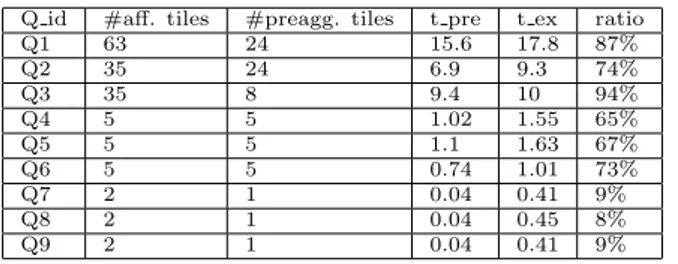
Table 2: Comparing query evaluation costs using pre-aggreated data and purely raw data.
Q id #aff. tiles #preagg. tiles t pre t ex ratio
Q1 63 24 15.6 17.8 87%
Q2 35 24 6.9 9.3 74%
Q3 35 8 9.4 10 94%
Q4 5 5 1.02 1.55 65%
Q5 5 5 1.1 1.63 67%
Q6 5 5 0.74 1.01 73%
Q7 2 1 0.04 0.41 9%
Q8 2 1 0.04 0.45 8%
Q9 2 1 0.04 0.41 9%
Table 2 compares the CPU cost required for the com-putation of the queries by using pre-aggregated data and purely raw data. The CPU cost was obtained by us-ing the time library of C++. The column #aff. tiles shows the number of tiles that would need to be consid-ered for computing the given query, whereas # preagg. tiles represents the number of pre-aggregates that can be used to compute the query. The columnt preshows the total CPU cost of computing the query considering pre-aggregated data. Finally, the columnt ex shows the time taken to execute the query entirely from raw data. The ratio column shows that the CPU time is always bet-ter when the computation of the queries considers pre-aggregated data.
6
Conclusions and Future Work
We have presented a framework for computing aggregate queries in raster image databases using pre-aggregated data. We distinguished among different types of pre-aggregates: inner, overlapped, and dominant. We showed that such a distinction is useful to identify those paggregates, from all potential candidates, that can re-duce the CPU cost required for the computation of the query. We proposed a cost-model to estimate the cost of using different pre-aggregates and thus select the best plan for evaluating the query in the presence of pre-aggregated data. The measurements on a real-life raster image dataset showed that the computation of the queries is always faster with our algorithms over straightforward methods. We focused on queries using the basic aggre-gate functions. This covers a large number of operations in Geo-raster applications but it remains the challenge to support more complex aggregate operations, e.g., scaling and edge-detection, which are under current investigation within our group.
References
[1] E. Adelson, C. Anderson, J. Bergen, P. Burt, and J. Odgen. Pyramid methods in image processing. RCA Engineer, (29-6):9, November/December 1984.
[2] P. Baumann. A database array algebra for spatio-temporal data and beyond,. The Fourth Interna-tional Workshop on Next Generation Information Technologies and Systems (NGITS), (Lecture Notes on Computer Science 1649, Springer Verlag):76–93, July 5-7 1999.
[3] A. Garcia-Gutierrez and P. Baumann. Modeling geo-raster operations with array algebra. InSeventh In-ternational Conference on Data Mining Workshops Proceedings, pages 607–612. ICDMW, 2007.