©2013 Science Publication
doi:10.3844/ajassp.2013.322.330 Published Online 10 (4) 2013 (http://www.thescipub.com/ajas.toc)
Corresponding Author: Noraini Ibrahim, Department of Industrial Computing and Modelling Mathematics,
Faculty of Computer Science and Information Systems, 81310, UTM Johor Bahru, Johor, Malaysia
PARTIAL LEAST SQUARES
REGRESSION BASED VARIABLES
SELECTION FOR WATER LEVEL PREDICTIONS
Noraini Ibrahim and Antoni Wibowo
Department of Industrial Computing and Modelling Mathematics,
Faculty of Computer Science and Information Systems, 81310, UTM Johor Bahru, Johor, Malaysia
Received 2012-05-25, Revised 2012-07-30; Accepted 2013-04-25
ABSTRACT
Floods are common phenomenon in the state of Kuala Krai, specifically in Kelantan-Malaysia. Every year, floods affecting biodiversity on this region and also causing property loss of this residential area. The residents in Kelantan always suffered from floods since the water overflows to the areas adjoining to the rivers, lakes or dams. Months, average monthly rainfall, temperature, relative humidity and surface wind were used as predictors while the water level of Galas River was used as response. The selection of suitable predictor variables becomes an important issue for developing prediction model since the analysis data uses many variables from meteorological and hydrogical departments.In this study, we conduct K-fold Cross-Validation (CV) to select the important variables for the water level predictions. A suitable prediction model is needed to forecast the water level in Galas River by adopting the Ordinary Linear Regression (OLR) and Partial Least Squares Regression (PLSR). However, we need to perform pre-processing data of the datasets since the original data contain missing data. We perform two types of pre-processing data which are using mean of the corresponding months (type I processing data) and OLR (type II pre-processing data) of missing data.Based on the experiment, PLSR is more suitable model rather than OLR for predicting the water level in Galas River and the use of the type I pre-processing data gives higher accuracy than the type II pre-processing data.
Keywords: Cross-Validation (CV), Ordinary Linear Regression (OLR), Partial Least Squares Regression (PLSR), Galas River, Water Level
1.
INTRODUCTION
Floods are common phenomenon which can be defined as the presence of excess of water in the place that is normally dry. Floods are often cited as being the most lethal of all natural disasters (Noji, 1997; Alexander, 1993; Jonkman and Kelman, 2005). The flooding of Malaysian rivers is mainly due to the high amount of rainfall in river basins because of the climate is greatly influenced by the monsoon winds. The worst flood in Malaysia was recorded in 1926 which has been described as having caused the most extensive damage to the natural environment. Subsequent major floods
were recorded in 1931, 1947, 1954, 1957, 1967 and 1971. Most countries in Malaysia suffer from floods during monsoon season especially in Kedah, Kelantan, Terengganu, Pahang and Johor. Kelantan is a state in the east coast of Peninsular Malaysia that has never missed a flooding event, which occurs every year during the northeast monsoon period.
a combination of physical factors such as elevation and its close proximity to the sea apart from heavy rainfall experienced during monsoon period. The severe floods all over Kelantan are resulted from heavy rainfall during the north east monsoon season especially in November and December. In order to facilitate the prediction of flooding in the river and the warning beforehand, this study aims to build a model on the relation between the selected predictors and the water level of Galas River by adopting the OLR and PLSR.
Kelantan state consists of more than 25 rivers and having seven major river basins that are Galas, Kelantan, Golok, Semerak, Pengkalan Chepa, Pengkalan Datu and Kemasin river basins. Kelantan River Basin is the biggest river basin in Kelantan and it drains a catchment area of about 12,000 km2 in north-east Malaysia including part of the National Park and flows northwards into the South China Sea (Rohasliney, 2010). The Kelantan River is about 248 km long and occupying more than 85% of the State of Kelantan. It divides into Galas and Lebir Rivers near Kuala Krai, about 100 km from the river mouth which means that Kelantan River is the main river while Galas and Lebir Rivers are the tributary rivers. For this study, we focused on one main
tributary of Kelantan River which is Galas River in Kuala Krai, Kelantan. Figure 1 shows the location of the study area which is Galas River.
The data for this analysis are collected from Water Resources Management and Hydrology Division and Malaysian Meteorological Department. It is noticed that the original data contain missing data. Missing data are common issue for data quality and most real datasets consist of missing data. There are four types of serious data quality problems in real datasets which are incomplete, redundant, inconsistent and noisy data. Based on our observation, the data has incomplete data which missing values in certain months. Due to the presence of missing data, the two methods can be inappropriate to be used directly for water level prediction, therefore, we need to perform a pre-processing data of the dataset. There are five factors that were identified and related to the level of the Galas River which can lead to the occurrence of flood phenomenon in Kuala Krai, Kelantan: (1) Months from January until December for 11 years starting from 2001 until 2011, (2) Monthly mean of rainfall, (3) Monthly mean of temperature, (4) Monthly mean of relative humidity and (5) Monthly mean of surface wind.
Different approaches for water level predictions can be found in hydrology science literature. The most common approaches for predicting the water level are stepwise regression (Zou et al., 2010), Artificial Neural Network (ANN) (Bustami et al., 2007) and ANN combined with PLSR (Shu et al., 2008). The previuos research on floods monitoring was conducted which is the utilizing of the GPS data for monitoring the severe flood in Kuala Krai Kelantan in order to detect the influence of heavy rainfall towards severe floods (Suparta et al., 2012). Another previuos research on the influence of groundwater flow systems towards climate change was reviewed to recommend the solutions that are more economical and enviromentally in managing the flooding water (Carrillo-Rivera and Cardona, 2012). A number of papers have previously reviewed on variables selection such as N-PLSR as empirical downscaling tool in climate change studies (Bergant and Kajfez-Bogataj, 2005) and application of PLSR as downscaling tool for Pichola lake in India (Goyal and Ojha, 2010). PLSR is successful mostly in chemometrics since the origin of PLSR lies in chemistry. It is useful when the factors are many highly collinear for constructing predictive models. In this study, we apply this method for variables selection to develope water level models. The following sections present an approach to the development of the water level models. Materials and methods are discussed in Section 2 while the results are described in Section 3. The discussion is reported in Section 4 and finally the conclusion is given in Section 5.
2.
MATERIALS
AND
METHODS
The linear regression model is given as in Equation (1) (Mevik and Cederkvist, 2004):
n 0 1
y= β +1 Xβ +ε (1)
where, y is an n×1 vector of observations on the response variable, X is an n×p matrix consisting of n observations and p predictors, β0 is an unknown constant, β1 is an p×1 vector of unknown regression coefficient,1n is an n×1 ones vector and ε is an n×1 vector of errors identically and independently distributed with mean zero and variance σ2>0, respectively.
2.1. Ordinary Linear Regression
OLR often being used in fitting models to make an observation which is applied by minimizing the sum of the squared residuals between the predicted and actual
response. When matrix X1 = [1n X] has full rank of p, the
OLR estimator of 1
T T 0
β= β( , β ) , say
T OLS OLS OLS
OLS 0 1 p
ˆ ˆ ˆ
βɵ = β[ ,β ,⋯,β ] , is estimated in Equation (2):
T 1 T
1 1 1
OLS
βɵ =(X X ) X y− (2)
The prediction of y is given in Equation (3):
ɵ
1 OLS
y=Xβɵ (3)
The model for OLR can be represented by Equation (4):
1 p
OLS0 OLS1 OLSp
ˆ ˆ ˆ
f (x)= β + β x + + β⋯ x (4)
where, x = [x1,x2,…,xp] T∈
RP
2.2. Partial Least Squares Regression
Partial Least Squares (PLS) has been proven to be an effective approach to solve the problems in chemometrics such as by predicting the bioactivity of molecules to facilitate discovery of novel pharmaceuticals. The PLS approach was originated around 1975 by Herman Wold for modeling the complicated datasets in terms of matrices blocks which called path models (Joreskog, 1982). The PLS method has been introduced in the chemical literature as an algorithm and it is only recently that its numerical and statistical properties have become more apparent (Stone, 1974). PLSR is a technique for modeling a linear relationship between a set of output variables (response)
n L
i i 1
{ }
y
= ∈R with L-dimensional responses and a set of input variables (regressors) n pi i 1
{x }= ∈R with p number of variables (Rosipal and Trejo, 2002). The data matrices X and y in this analysisare assumed to be centered as a first step to perform PLSR.
2.3. Partial Least Squares Regression Using
SIMPLS Algorithm
SIMPLS algorithm was used to compute the regression coefficient in order to find the model for predicting water level in Dungun River of Terengganu. SIMPLS algorithms work very well, resistant to be more appropriate, fast, easy to implement and simple to tune (Bennett and Embrechts, 2003). In PLSR approach, we need to obtain the PLSR estimator, say BˆPLSR
T PLSR1 PLSR 2 PLSRp
ˆ ˆ ˆ
[B , B , , B ] ,
= ⋯ and it starts with computing
the cross-product of (Jong, 1993; Ibrahim and Wibowo, 2012) as shown in Equation (5):
T
S=X y (5)
Then, the computing of the iteration is followed starting from 1 until A latent variables where A is determined in advanced and 1≤A ≤ p. The algorithm of SIMPLS is given as follows:
For a =1to A:
• If a = 1, then do the singular value decomposition (svd) of S: [u, u, v] = svd (S)
Otherwise, if a > 1, we compute the svd of:
T 1 T
[u,s, v]=svd (S−P(P P) P S)−
• Get weights for rwhich is the first singular vector: r = u (:, 1)
• Compute the scores: t = Xr
• Compute the loadings: p = XT t/(tTt)
• The vector r, t and p are stored into R, T and P respectively
The last step is computing a regression coefficient can be shown in Equation (6):
T 1 T
PLSR ˆ
B =R(T T) T y− (6)
Then, the estimate of PLSR is given in Equation (7):
ɵ ˆPLSR
y=XB (7)
The model for PLSR can be represented by Equation (8):
1 1 p p
PLSR1 PLSRp
ˆ ˆ
g(x)= +y B (x −x )+ +⋯ B (x −x ) (8)
where, yis the mean of response yi and xpis the mean of observation data of xp.
2.4. Evaluating the Quality of the Prediction
The quality of the prediction is evaluated using A latent variables, ɵyi and yi (Helland, 1988; Ibrahim and Wibowo, 2012). CV technique is used to estimate the prediction capacity and the data are separated between the training data set to build the model and testing data set to test the model. The CV is applied in three cases which are in performance estimation, model selection and tuning learning model parameters. In this study, CV is used in predictors’ selection and model selection for predicting water level of Dungun River. The CV is a statistical method to evaluate the algorithms by dividing the data into two segments which are for training and validation and the basic form of cross-validation is K-fold CV. The idea for CV was originated in the 1930s (Larson, 1931; Refaeilzadeh et al., 2008; Ibrahim and Wibowo, 2012). In 1970s, CV was employed as means for choosing proper model parameters, as opposed to using cross-validation purely for estimating model performance (Geisser, 1975; Sjgstrgm et al., 1983; Ibrahim and Wibowo, 2012).
2.5. Data
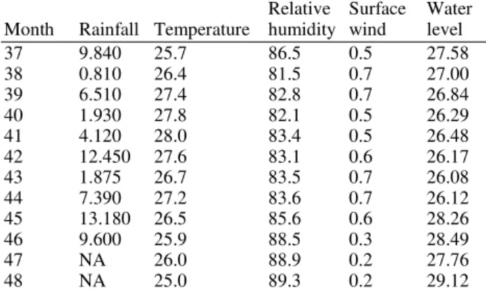
As predictors in predicting water level of Galas River, months (x1), average monthly rainfall (x2), temperature (x3), relative humidity (x4) and surface wind (x5) were identified and related to the occurrence of flood phenomenon in Kuala Krai, Kelantan. Observed predictors and response for the period 2001-2011 were extracted from the Water Resources Management and Hydrology Division in Kuala Lumpur and Malaysian Meteorological Department in Selangor. Variable selection is performed to select the suitable predictors in predicting the water level based on the MSECV of OLR and PLSR. It is noted that the data consist of missing values for rainfall and water level and we performed cleaning data to replace these missing values. The data are separated into two sub data which are 120 data for developing models and variables selection using 10-fold CV and 12 data for validating the models. The data that were used in this analysis are shown in Table 1.
2.6. Original Data
The data set is cover from January until December for 11 years and yet it has shown a total of 132 data.
Table 1-4 describe the predictors and response used over training period in predicting water level of Galas River. The first column, second column, third column, fourth column, fifth column and sixth column represent months, rainfall, temperature, relative humidity, surface wind and water level data, respectively. They show the raw data and 47th month is in November 2004 and the NA values means that there are missing values of rainfall in November and December 2004.
2.7. Pre-Processing Data
Data preprocessing is the process that was performed to the original data in order to prepare it for next processing procedure. Thus, it will transform the data into the format that more effective according to our purpose of analysis. Data preprocessing is important since the real world data normally are noisy which are containing errors and outliers. There are five tasks in performing data preprocessing which are data cleaning, data integration, data transformation, data reduction and data discretization. For this analysis, we performed two types of data cleaning which are using mean of the corresponding months throughout 11 years and OLR to replace the missing values of rainfall and water level.
Table 1. Details of the data Station Period Data
Kuala Krai 2001-2011 Monthly 24 h Mean Temperature Monthly 24 h
Mean relative humidity Monthly mean surface wind Dabong 2001-2011 Monthly mean
rainfall and water level
Table 2. The snapshot of original data of Galas River
Relative Surface Water Month Rainfall Temperature humidity wind level 37 9.840 25.7 86.5 0.5 27.58 38 0.810 26.4 81.5 0.7 27.00 39 6.510 27.4 82.8 0.7 26.84 40 1.930 27.8 82.1 0.5 26.29 41 4.120 28.0 83.4 0.5 26.48 42 12.450 27.6 83.1 0.6 26.17 43 1.875 26.7 83.5 0.7 26.08 44 7.390 27.2 83.6 0.7 26.12 45 13.180 26.5 85.6 0.6 28.26 46 9.600 25.9 88.5 0.3 28.49 47 NA 26.0 88.9 0.2 27.76 48 NA 25.0 89.3 0.2 29.12
Table 3. The snapshot of pre-processing data of galas river using type I pre-processing data
Relative Surface Water Month Rainfall Temperature humidity wind level 37 9.840 25.7 86.5 0.5 27.58 38 0.810 26.4 81.5 0.7 27.00 39 6.510 27.4 82.8 0.7 26.84 40 1.930 27.8 82.1 0.5 26.29 41 4.120 28.0 83.4 0.5 26.48 42 12.450 27.6 83.1 0.6 26.17 43 1.875 26.7 83.5 0.7 26.08 44 7.390 27.2 83.6 0.7 26.12 45 13.180 26.5 85.6 0.6 28.26 46 9.600 25.9 88.5 0.3 28.49 47 12.750 26.0 88.9 0.2 27.76 48 163.280 25.0 89.3 0.2 29.12
Table 4. The snapshot of pre-processing data of Galas River using type ii pre-processing data
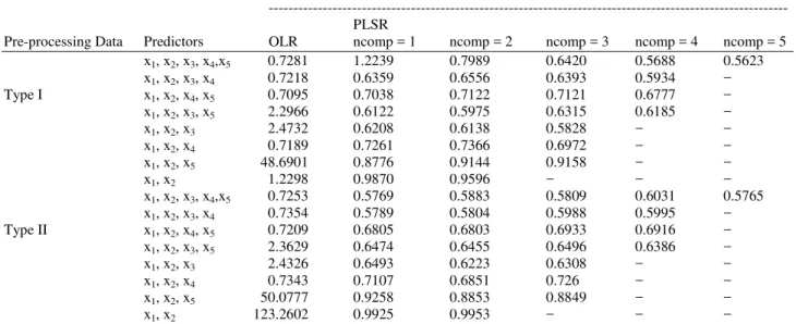
Table 5. Msecv for variable selection of Galas River MSECV
--- PLSR
Pre-processing Data Predictors OLR ncomp = 1 ncomp = 2 ncomp = 3 ncomp = 4 ncomp = 5 x1, x2, x3, x4,x5 0.7281 1.2239 0.7989 0.6420 0.5688 0.5623 x1, x2, x3, x4 0.7218 0.6359 0.6556 0.6393 0.5934 − Type I x1, x2, x4, x5 0.7095 0.7038 0.7122 0.7121 0.6777 − x1, x2, x3, x5 2.2966 0.6122 0.5975 0.6315 0.6185 − x1, x2, x3 2.4732 0.6208 0.6138 0.5828 − − x1, x2, x4 0.7189 0.7261 0.7366 0.6972 − − x1, x2, x5 48.6901 0.8776 0.9144 0.9158 − −
x1, x2 1.2298 0.9870 0.9596 − − −
x1, x2, x3, x4,x5 0.7253 0.5769 0.5883 0.5809 0.6031 0.5765 x1, x2, x3, x4 0.7354 0.5789 0.5804 0.5988 0.5995 − Type II x1, x2, x4, x5 0.7209 0.6805 0.6803 0.6933 0.6916 − x1, x2, x3, x5 2.3629 0.6474 0.6455 0.6496 0.6386 − x1, x2, x3 2.4326 0.6493 0.6223 0.6308 − − x1, x2, x4 0.7343 0.7107 0.6851 0.726 − − x1, x2, x5 50.0777 0.9258 0.8853 0.8849 − −
x1, x2 123.2602 0.9925 0.9953 − − −
2.8. Pre-processing Data Using Mean of the
Corresponding Months
For this subsection, we used mean of the corresponding months which is represented by type I pre-processing data to replace these missing values. For example, NA value of rainfall in November and December 2004 for Galas River are replaced by the means of the corresponding months throughout 11 years. Table 4 presents the snapshot of the pre-processing data using mean of the corresponding months for Galas River.
2.9. Pre-processing Data Using Ordinary Linear
Regression
The second type of cleaning data that we used is OLR and we represent it as type II pre-processing data. We performed OLR to replace the missing values of the dataset in Galas River. Table 3 shows the snapshot of the pre-processing data using OLR for Galas River.
The model to replace the missing value of the water level for Galas River is given in Equation (9):
1 1
OLR WL1
f (x )=26.5767+0.0135x (9)
The model to replace the missing values of the rainfall for Galas River is represented by Equation (10):
1 1
OLR RF1
f (x )=6.4736+0.0021x (10)
2.10. Selection of Predictors
The selection of appropriate predictors is one of the most important steps in predicting the water level of Galas River. The predictors are chosen based on the smallest value of MSECV and the result is compared between two types ofpre-processing data which are type I pre-processing data and type II pre-processing data. It can be seen from Table 5 that five predictor variables namely months (x1), average monthly rainfall (x2), temperature (x3), relative humidity (x4) and surface wind (x5) with type I pre-processing data have their lowest value of MSECV when ncomp is equals to five. Hence, these variables are used in the water level predictions.
3. RESULTS
3.1. Models Development
The models for water level predictions of Galas River were developed using OLR and PLSR. The results were compared between these two approaches and between two types of pre-
processing data.
3.2. Ordinary Linear Regression
using type I pre-processing data of Galas River is given by Equation (11):
1 2 3 4 5
1 2
3
4 5
OLRGalasI
f (x , x , x , x , x ) 31.6220
0.0038x 0.0323x
0.5443x
0.1165x 0.4555x =
+ +
− +
−
(11)
The prediction model for water level using type II pre-processing data of Galas River is given in Equation (12).
1 2 3 4 5 1
2
3
4 5
OLRGalasII
f (x , x , x , x , x ) 30.0678 0.0036x
0.0309x
0.5085x
0.1233x 0.3873x
= +
+
− +
−
(12)
3.3. Partial Least Squares Regression:
PLSR is another method that we use in this experiment in order to get the prediction model and the results based on these two methods are being compared between original data and cleansing data. Validation method is used for choosing number of components of PLS and the model with the lowest MSECV is considered to be the optimal one.
The prediction model for water level of Galas River using type I pre-processing data is represented by Equation (13):
PLSRGalasI 1 2 3 4 5
1 2
3
4 5
g (x , x , x , x , x ) 33.1985
0.0037x 0.0340x
0.5712x
0.1064x 0.4552x
= +
+ −
+ −
(13)
The prediction model for water level using type II pre-processing data of Galas River is given in Equation (14):
1 2 3 4 5
1 2
3
4 5
PLSRGalasII
g (x , x , x , x , x ) 31.5444
0.0036x 0.0324x
0.5340x
0.1139x 0.3889x
= +
+ −
+ −
(14)
3.4. Model Selection
In this study, we will restrict ourselves to the common variants of CV called K-fold CV, where the calibration objects are divided in k segments and for this experiment we use k = 10 (Breiman, 1984; Wiklund et al., 2007; Ibrahim and Wibowo, 2012). The selected number of components using k-fold CV correctly find this range, the actual value of the number of components is immaterial as long as the prediction error is close to its minimum (Wiklund et al., 2007; Ibrahim and Wibowo, 2012). We used 10-fold CV to obtain the appropriate model for predicting water level at Galas River of Kuala Krai using two types of pre-processing data. The data were analyzed using OLR and PLSR and the results are compared between these two types of pre-processing data to obtain a better model according to lowest value of MSECV.
4. DISCUSSION
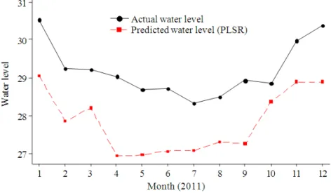
Table 6 illustrates the comparison of MSECV for Water Level in Galas River using 10-fold CV of OLR and PLSR. From this result, it shows that PLSR with type I pre-processing data of ncomp equals to 5 has the smallest MSECV. Therefore, this PLSR is considered as the best model. Figure 2 shows the comparison between actual and prediction monthly water level for Galas River with test data in 2011 using type I pre-processing data and Fig. 3 presents the comparison between predicted and actual water level in Galas River with test data using type II pre-processing data. From these graph, it is clear that the use of type I pre-processing data achieves closer agreement between actual and predicted water level rather than using type II pre-processing data.
Table 6. Msecv for variables selection of Galas River MSECV
--- PLSR
--- Pre-processing data OLR ncomp = 1 ncomp = 2 ncomp = 3 ncomp = 4 ncomp = 5
Type I 0.7281 1.2239 0.7989 0.642 0.5688 0.5623
Fig. 2. A comparison between actual and prediction monthly water level for Galas River with test data of 2011 using type I pre-processing data
Fig. 3. A comparison between actual and prediction monthly water level for Galas River with test data of 2011 using type II pre-processing data
5. CONCLUSION
In Kuala Krai district, rising water levels of the river become critical issues since it can induce flood and destroy a lot of things. We had compared between two types of pre-processing data which are type I and type II pre-processing data using OLR and PLSR approaches for variables selection and model selection. The experiment had shown that PLSR is a suitable method in variables selection and model development since it give higher accuracy than using OLR. Our further
research will focus on the use of nonlinear method and compare them to PLSR model.
6.
ACKNOWLEDGEMENT
Zamalah scholarship for supporting her master by research program.
7.
REFERENCES
Alexander, D.E., 1993. Natural Disasters. 1st Edn., Springer Science and Business, New York, ISBN-10: 0412047411, pp: 632.
Bennett, K.P. and M.J. Embrechts, 2003. An optimization Perspective on Kernel Partial Least Squares Regression. In: Advances in Learning Theory: Methods, Models and Applications, Suykens, J.A.K. (Ed.), IOS Press, Amsterdam, ISBN-10: 1586033417, pp: 227-250.
Bergant, K. and L. Kajfez-Bogataj, 2005. N-PLS regression as empirical downscaling tool in climate change studies. Theoritical Applied Climatol., 81: 11-23. DOI: 10.1007/s00704-004-0083-2
Breiman, L., 1984. Classification and Regression Trees. 1st Edn., Wadsworth International Group, Belmont, Calif., ISBN-10: 0534980538, pp: 358.
Bustami, R., N. Bessaih, C. Bong and S. Suhaili, 2007. Artificial neural network for precipitation and water level predictions of Bedup River. IAENG Int. J. Comput. Sci.
Carrillo-Rivera, J.J. and A. Cardona, 2012. Groundwater flow systems and their response to climate change: A need for a water-system view approach. Am. J.
Environ. Sci., 8: 220-235. DOI:
10.3844/ajessp.2012.220.235
Davison, A.C. and D.V. Hinkley, 1997. Bootstrap Methods and their Application. 2nd Edn., Cambridge University Press, Cambridge, ISBN-10: 0521574714, pp: 582.
Geisser, S., 1975. The predictive sample reuse method with applications. J. Am. Stat. Assoc., 70: 320-328. DOI: 10.1080/01621459.1975.10479865
Goyal, M.K. and C.S.P. Ojha, 2010. Application of PLS-regression as downscaling tool for pichola lake basin in India. Int. J. Geosci., 1: 51-57. DOI: 10.4236/ijg.2010.12007
Helland, I.S., 1988. On the structure of partial least squares regression. Commun. Stat. Elem. Simul.
Comput., 17: 581-607. DOI:
10.1080/03610918808812681
Ibrahim, N. and A. Wibowo, 2012. Predictions of water level in Dungun River Terengganu using partial least squares regression. Int. J. Basic Applied Sci., 12: 1-7. Jong, S.D., 1993. SIMPLS: An alternative approach to partial least squares regression. Chemometr. Intell. Laboratory Syst., 18: 251-263. DOI: 10.1016/0169-7439(93)85002-X
Jonkman, S.N. and I. Kelman, 2005. An analysis of the causes and circumstances of flood disaster deaths. Disasters, 29: 75-97. DOI: 10.1111/j.0361-3666.2005.00275.x
Joreskog, K.G., 1982. Systems under Indirect Observation. 1st Edn., North-Holland, Amsterdam, ISBN-10: 044486301X, pp: 636.
Larson, S.C., 1931. The shrinkage of the coefficient of multiple correlation. J. Educ. Phychol., 22: 45-55. DOI: 10.1037/h0072400
Mevik, B.H. and H.R. Cederkvist, 2004. Mean Squared Error of Prediction (MSEP) estimates for Principal Component Regression (PCR) and Partial Least Squares Regression (PLSR). J. Chemometr., 18: 422-429. DOI: 10.1002/cem.887
Noji, E.K., 1997. The Public Health Consequences of Disasters. 1st Edn., Oxford University Press, USA., ISBN-10: 0195095707, pp: 468.
Refaeilzadeh, P., L. Tang and H. Liu, 2008. Cross-Validation. Arizona State University.
Rohasliney, H., 2010. Status of river fisheries in Kelantan, Peninsular Malaysia, Malaysia. World Acad. Sci., Eng. Technol., 65: 829-834.
Rosipal, R. and L.J. Trejo, 2002. Kernel partial least squares regression in reproducing kernel hilbert space. J. Mach. Learn. Res., 2: 97-123.
Shu, L., G. Dong, L. Liu, Y. Tao and M. Wang, 2008. Water level variation and prediction of the Pingshan Sinkhole in Guizhou, Southwestern China. Am. Soc. Civil Eng. DOI: 10.1061/41003(327)40
Sjgstrgm, M., S. Wold, W. Lindberg, J.A. Persson and H. Martens, 1983. A multivariate calibration problem in analytical chemistry solved by partial least-squares models in latent variables. Anal. Chim. Acta, 150: 61-70. DOI: 10.1016/S0003-2670(00)85460-4 Stone, M., 1974. Cross-validatory choice and assessment of
statistical predictions. J. Royal Stat. Soc., 36: 111-147. Suparta, W., J. Adnan and M.A.M. Ali, 2012. Monitoring
of GPS precipitable water vapor during the severe flood in Kelantan. Am. J. Applied Sci., 9: 825-831. DOI: 10. 384/ajassp.2012.825.831
Wiklund, S., D. Nilsson, L. Eriksson, M. Sjostrom and S. Wold et al., 2007. A randomization test for PLS component selection. J. Chemom., 21: 427-439. DOI: 10.1002/cem.1086
Zou, Y., W. Zhou and M. Zhong, 2010. A model on the relation between the rainfall in Poyang Lake Basin and its Water Level. Proceedings of the 4th International Conference on Bioinformatics and Biomedical Engineering, Jun. 18-20, IEEE Xplore
Press, Chengdu, pp: 1-4. DOI: