Metrics of hurricane-ocean interaction: vertically-integrated or vertically-averaged ocean temperature?

(1)

OSD

6, 909–951, 2009

Metrics of hurricane-ocean

interaction

J. F. Price

Title Page

Abstract Introduction

Conclusions References

Tables Figures

◭ ◮

Back Close

Full Screen / Esc

Printer-friendly Version

Interactive Discussion Ocean Sci. Discuss., 6, 909–951, 2009

www.ocean-sci-discuss.net/6/909/2009/

Ocean Science Discussions

Papers published inOcean Science Discussionsare under open-access review for the journalOcean Science

Metrics of hurricane-ocean interaction:

vertically-integrated or

vertically-averaged ocean temperature?

J. F. Price

Woods Hole Oceanographic Institution, Woods Hole, Massachusetts 02543, USA

Received: 1 April 2009 – Accepted: 15 April 2009 – Published: 5 May 2009

Correspondence to: J. F. Price (jprice@whoi.edu)

(2)

OSD

6, 909–951, 2009

interaction

J. F. Price

Title Page

Tables Figures

◭ ◮

Back Close

Full Screen / Esc

Interactive Discussion

Abstract

The ocean thermal field is often represented in hurricane-ocean interaction by a metric termed the upper Ocean Heat Content (OHC), the vertical integral of ocean tempera-ture in excess of 26◦C. High values of OHC have proven useful for identifying ocean regions that are especially favorable for hurricane intensification. Nevertheless, it is 5

argued here that a more direct and robust metric of the ocean thermal field may be afforded by a vertical average of temperature, in one version from the surface to 100 m, a typical depth of vertical mixing by a mature hurricane. OHC and the depth-averaged temperature, dubbed T₁₀₀, are well correlated over the deep open ocean in the high range of OHC, OHC≥75 kJ cm−2. They are poorly correlated in the low range of OHC,

10

≤50 kJ cm−2, in part because OHC is degenerate when evaluated on cool ocean tem-peratures≤26◦C. OHC and T₁₀₀ can be qualitatively different also over shallow conti-nental shelves: OHC will generally indicate comparatively low values regardless of the ocean temperature, whileT₁₀₀ will take on high values over a shelf that is warm and upwelling neutral or negative, since there will be little cool water that could be mixed 15

into the surface layer. Some limited evidence is that continental shelves may be re-gions of comparatively small sea surface cooling during a hurricane passage, but more research is clearly required on this important issue.

1 Hurricanes and the ocean

Hurricanes draw energy from the ocean in the form of sensible and latent heat (en-20

(3)

OSD

6, 909–951, 2009

interaction

J. F. Price

Title Page

Tables Figures

◭ ◮

Back Close

Full Screen / Esc

Interactive Discussion ocean temperature difference. This hurricane-induced cooling of the sea surface must

reduce the hurricane-ocean heat flux and thus the hurricane intensity to some degree (Bender et al., 1993; Schade and Emanuel, 1999; Cione and Uhlhorn, 2003). The object of this study is an improved representation of the ocean thermal conditions that contribute to greater or lesser cooling of the sea surface by a hurricane, with the long 5

range goal being improved forecasting of hurricane-ocean interaction.

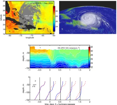
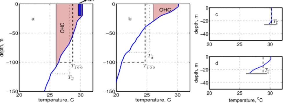
In what follows the pre-hurricane (initial) temperature fieldT_i(x, y, z) is presumed known in the sense of being observable by more or less routine in situ and remote ocean observing systems. The SST of a hurricane wake, T_w(x, y, z=0), is also ob-servable by remote sensing methods, as in Fig. 1a, but of course only after the fact, 10

i.e., after a hurricane passage. The ocean side of the forecasting problem is to predict the SST under a hurricane, T_h(x, y, z=0) (Cione and Uhlhorn, 2003). This T_h is not routinely observable because of the heavy clouds and rain of the hurricane itself. In later Sects. 2 and 3, the emphasis will be on modelling and forecasting the observable wake temperature, Tw, and then on closing we will come back to consider the

rela-15

tionship betweenT_h, T_i andT_w suggested by a handful of in situ observations, roughly

Th≈(Ti+Tw)/2 (D’Asaro et al. (2007) and Fig. 1c and d).

The ocean models of a forecasting system can take one of several forms. In the first place, ocean dataT_i(x, y, z) may be combined with three-dimensional (3-D) ocean circulation, mixing and wave models that may in turn be coupled to a weather prediction 20

model. These comprehensive, coupled air-sea models can be used to make detailed forecasts of specific storms (Ginis, 2002; Bender et al., 2007; Chen et al., 2007) and will soon be a primary forecast tool in some weather centers. At the other extreme of complexity, the same ocean data and an understanding of the salient ocean mixing and thermodynamics might also be combined into a mappable, two-dimensional (x, y) 25

(4)

Tri-OSD

6, 909–951, 2009

interaction

J. F. Price

Title Page

Tables Figures

◭ ◮

Back Close

Full Screen / Esc

Interactive Discussion nanes, 2003; DeMaria et al., 2005; and see especially the informative, recent review

by Mainelli et al., 2008). The history of OHC, described briefly below, includes some notable successes that have served to demonstrate an important role for ocean obser-vations and ocean models within hurricane forecasting. But there are also persistent anomalies that seem to indicate room for improvement.

5

1.1 The first ocean metric, upper ocean heat content

OHC is defined in this hurricane-ocean context as the vertical integral of ocean tem-perature in excess of 26◦C,

OHC(x, y)=ρ_oC_p

Z0

Z26

(T_i(x, y, z)−26)d z, (1)

where the lower limit of integration is the depth of the 26◦C isotherm. The leading fac-tors,ρo=1025 kg m

−3

andCp=4.0×103J kg −1

are sea water density and heat capacity, usually taken as constants. The reference temperature, 26◦C, is an average (dry bulb) temperature in the subtropical atmospheric boundary layer and soTi(x, y, z=0)−26 is

10

a measure of the thermal disequilibrium between the atmosphere and the initial state of the ocean. It is well-known that 26◦C is also the approximate, lower range of SST at which hurricanes are observed to form (Gray, 1968). Warm or cool as used here will then be with respect to 26◦C. In the usual case that ocean temperature is monton-ically increasing toward the surface, waters with temperature less than 26◦C make no 15

contribution to OHC.1

1

(5)

OSD

6, 909–951, 2009

interaction

J. F. Price

Title Page

Tables Figures

◭ ◮

Back Close

Full Screen / Esc

Interactive Discussion OHC was not derived from theory or from an ocean model so much as it was

con-structedad hocon the intuitive, reasonable basis that if hurricane-ocean heat exchange is important to a hurricane, then oceanic regions having larger or smaller OHC should be more or less favorable for hurricane formation or intensification (Leipper and Volge-nau, 1972) (hereafter just intensification). There will be a discussion of mechanisms in 5

what follows, but for now we note that this expectation has been largely borne out in forecasting practice and in statistical analysis (hindcast) within the high range of OHC, roughly OHC≥60 kJ cm−2(Goni and Trinanes, 2003; Scharoo et al., 2006; McTaggart-Cowan et al., 2007; Lin et al., 2008; Mainelli et al., 2008; see also Sun et al., 2006). OHC takes on the largest values,≥100 kJ cm−2, over oceanic regions having a

com-10

paratively thick, warm surface layer, often in association with a subtropical gyre interior or an associated western boundary current system, the Kuroshio or the Gulf of Mex-ico’s Loop Current (Shay et al., 2000). An important correlation between these high OHC features and hurricane intensification has been found in late summer conditions

can be almost completely avoided by use of potential enthalpy (McDougall, 2003). A much bigger conservation error may arise from the lower limit of integration for OHC, the depth of the 26◦C isotherm,Z₂₆. In the presence of vertical mixing nearZ₂₆, which occurs commonly (Fig. 1b and 1c, and D’Asaro et al., 2007), this lower limit is not a material surface whose motion would be connected by continuity with the surrounding fluid. To appreciate the consequence, imagine that vertical mixing within the ocean surface layer (no hurricane-ocean heat flux) acts

to cool the surface layer, eventually below 26◦C. The depthZ₂₆will move upward through the

water column, and OHC will vanish whenZ₂₆reaches the sea surface, i.e., as the surface layer

cools below 26◦C. This decrease of OHC in a given column is not necessarily balanced by a

(6)

OSD

6, 909–951, 2009

interaction

J. F. Price

Title Page

Tables Figures

◭ ◮

Back Close

Full Screen / Esc

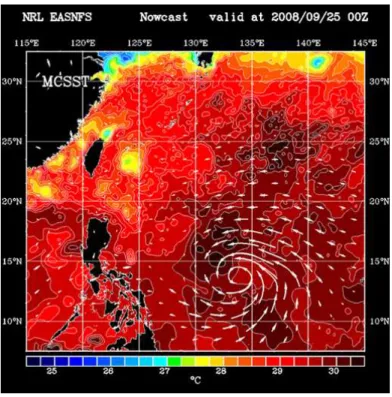
Interactive Discussion in which the pre-hurricane SST field is often quasi-uniform horizontally (Figs. 2 and

3). Wide experience has thus shown that OHC provides significant information on the ocean thermal field beyond that provided by the SST field alone.

There are also observations that do not appear to fit within the OHC framework. At one level this is not unexpected; ocean thermal conditions, no matter how represented, 5

are not the sole nor necessarily the most important determinant of hurricane intensity. Large-scale wind and humidity distributions are at least as important, and internal vari-ability occurs within hurricanes on small spatial and time scales that are very difficult to predict (Marks et al., 1998). One notable, apparent anomaly has real consequences for forecasting, viz., the correlation between hurricane intensity and OHC found in the high 10

range of OHC disappears within the low range of OHC, 0≤OHC≤60 kJ cm−2(Mainelli et

al., 2008). Thus, while high values of OHC are found to favor hurricane intensification, low values of OHC evidently have very little if any significant, consistent effect, either positive or negative. The apparent lack of sensitivity to low range OHC could be a prop-erty of the atmosphere, of course, but on the other hand, case studies have shown that 15

a sufficiently cool sea surface can have a pronounced damping effect upon hurricane intensity (Monaldo et al., 1997; Walker et al., 2005). The loss of correlation between hurricane intensity and OHC at low OHC is considered in some detail in Sects. 3.1.2 and 3.2.1 and the conclusion will be that OHC does not bear a consistent relationship to any SST in cool, deep ocean conditions or in shallow water. The upshot is that OHC 20

does not appear to be an ideal metric of hurricane-ocean interaction in these condi-tions. To be fair to Leipper and Volgenau (1972), this amounts to holding OHC up to a wider and higher standard than they had envisioned. However, maps of OHC (Goni and Trinanes, 2003) and statistical analyses using OHC as the ocean metric (DeMaria et al., 2005; Mainelli et al., 2008) necessarily show and average over all oceanic regions 25

(7)

OSD

6, 909–951, 2009

interaction

J. F. Price

Title Page

Tables Figures

◭ ◮

Back Close

Full Screen / Esc

1.2 The goal and the plan of this paper

The goal of this work is to enhance the value of ocean observations and ocean models that might be used within a hurricane forecasting or analysis scheme. The scope is limited to the ocean half of hurricane-ocean interaction, and the object is a new, rationalized ocean metric. The approach will be to build upon the extensive history 5

of OHC reviewed above, while also making use of guidance from 3-D ocean models and ocean process studies that were unavailable when OHC was first proposed. The starting point for a new metric is a review of the processes that cause sea surface cooling by a hurricane, Sect. 2. This leads to the hypothesis that a vertical average of upper ocean temperature is a more direct metric for SST underneath a hurricane than 10

is OHC, a vertical integral of ocean temperature. The consequences of averaging (the new metric) vis a vis integrating (OHC) are explored in Sect. 3; Sect. 3.1 considers the deep, open ocean, and Sect. 3.2 considers a continental shelf. A summary and remarks on possible future research on this topic are in the concluding Sect. 4.

2 The mechanisms of hurricane-ocean interaction

15

It goes almost without saying that upper ocean ’heat’ content is not a substance this is transferred from the ocean into the atmosphere simply by contact. And specifically, high OHC does not by itself insure that there will be a high heat flux from the ocean into the atmosphere. A thermal disequilibrium between the ocean and hurricane, and thus the SST, must be involved as an intermediary. The route to a new ocean metric 20

begins from this point of view and requires only two premises. Premise 1, which more or less repeats this obvious point, but is nevertheless useful for keeping focus, is that

(8)

OSD

6, 909–951, 2009

interaction

J. F. Price

Title Page

Tables Figures

◭ ◮

Back Close

Full Screen / Esc

Interactive Discussion Subsurface ocean temperature may be important indirectly, but only to the extent that

it contributes to setting the SST. The SST under a hurricane is singled out simply because it coincides with the highest winds and thus with the greatest potential for hurricane-ocean heat exchange (Cione and Uhlhorn, 2003). Assuming that the initial temperature fieldTi(x, y, z) is known (observed), then the task is to forecast the cooling

5

of SST that occurs under a hurricane (taking the hurricane perspective, as in Fig. 1a) or during a hurricane passage (from the ocean perspective, Fig. 1c). (It might be added that P1 seems to elide a role for sea state out of ignorance, not conviction.)

2.1 Sea surface cooling processes

The sea surface underneath a hurricane is cooled by two distinct processes, by heat 10

exchange across the sea surface noted above, and by vertical, turbulent mixing of cooler water upward into the surface layer (Price, 1981; Jacob et al., 2000; D’Asaro et al., 2007). If induced sea surface cooling was due mainly to hurricane-ocean heat exchange, then OHC would be an appropriate metric for representing the ocean thermal field. Two lines of evidence indicate otherwise. In the pioneering study 15

by Leipper and Volgenau (1972) it was noted that the large values of OHC found over much of the deep, subtropical oceans are far in excess of the time-integrated heat flux to a given hurricane, often by a factor of 10 or more (noted also by Cione and Uhlhorn, 2003, and by Mainelli et al., 2008). In a later Sect. 3.2, the net (time-integrated) heat flux to a single hurricane is estimated as Qnet≈4×10

7

J m−2=4 kJ cm−2 (Fig. 5). This 20

net heat flux will cool a water column that is 10 m thick by only about 1◦C (Fig. 5). Thus, even a rather shallow, warm continental shelf will have a greater heat content, as estimated by OHC, than will be absorbed by a single hurricane. Over the deep, open ocean the SST cooling caused by heat loss is O(0.1) ◦C, and in most respects negligible. On this basis alone it would seem unlikely that OHC per se sets a limit on 25

(9)

OSD

6, 909–951, 2009

interaction

J. F. Price

Title Page

Tables Figures

◭ ◮

Back Close

Full Screen / Esc

Interactive Discussion ocean thermal field in some specific conditions, e.g., the warm, deep ocean conditions

emphasized by Leipper and Volgenau (1972) (Sect. 3.1.1).

A number of subsequent, upper ocean field studies and model studies have found that the main process that cools the sea surface underneath a hurricane is vertical, turbulent mixing (Price, 1981; Bender et al., 1993; Sanford et al., 2007; D’Asaro et al., 5

2007). Thus the sea surface may cool significantly without there being an appreciable change in the upper ocean heat content (suitably chosen, footnote 1). The temperature profiles of Fig. 1d are an example; during the passage of Hurricane Frances (2004) the surface temperature cooled by about 2.5◦C as the temperature profile became quasi-homogeneous over roughly the upper 100 m. A comparison of pre- and post-hurricane 10

temperature profiles shows that the net cooling (temperature change times thickness) caused by vertical mixing near the surface is approximately balanced by the net warm-ing caused by vertical mixwarm-ing in the upper thermocline (this warmwarm-ing is not of direct interest here, but see Sriver and Huber, 2008). Detailed, quantitative studies of the up-per ocean heat budget have found that the ratio of the heat flux due to vertical mixing 15

compared to the hurricane-ocean heat exchange is O(10) in deep water cases (Ja-cob et al., 2000; Cione and Uhlhorn, 2003; D’Asaro et al., 2007), consistent with the observation noted above that the net heat loss is small compared to the cooling of the surface layer. The ocean side of hurricane-ocean interaction can then be summa-rized in Premise 2: While hurricane-ocean heat exchange may be very important to a 20

hurricane, nevertheless

P2: The large amplitude, 1–4◦C, cooling of the sea surface during a hurri-cane passage is due mainly to vertical mixing of cooler water into the ocean surface layer.

The dominant role of vertical mixing has been understood for some time. The present 25

(10)

OSD

6, 909–951, 2009

interaction

J. F. Price

Title Page

Tables Figures

◭ ◮

Back Close

Full Screen / Esc

2.2 A new ocean metric, depth-averaged temperature

Given P1 and P2, it follows that a metric intended to represent the ocean thermal field within hurricane-ocean interaction should account first of all for the sea surface cooling e_ffect of vertical mixing caused mainly by the very high winds of a hurricane, and secondarily for hurricane-ocean heat exchange. Vertical mixing is equivalent to vertical averaging, and this leads to the first of two hypotheses advanced in this paper: H1: The appropriate metric of the ocean thermal field is a vertical average of the initial (pre-hurricane) ocean temperature,

T_d(x, y)=1

d

Z0

−d

Ti(x, y, z)d z, (2)

whered is the depth of vertical mixing caused by a hurricane, i.e., the surface mixed-layer thickness.

The depthd has to be predicted ifT_d is to be predicted, and two methods for doing that are discussed below. The depth-averaged temperature,T_d , is then an estimate of 5

the mixed-layer temperature in the wake,T_d(x, y)≈T_w(x, y, z=0) and is intended to be an approximation of the SST computed by the 3-D hurricane-ocean models of the kind noted in Sect. 1.1. Aside from skin effects that are presumably very small, this T_d is essentially the sea surface temperature.

Given that SST only decreases during a hurricane passage, the interpretation of 10

T_d is straightforward. High values, say T_d≥28◦C, would indicate even slightly higher

SST during a hurricane passage and thus an ocean thermal field that is favorable for hurricane intensification. On the other hand, low values, sayT_d≤24◦C, would just as clearly indicate low values of SST during a hurricane passage, and so an ocean thermal field that was unfavorable (or much less favorable) for intensification.

15

If there is a comparatively small temperature contrast in the water column above

z=−d that is mixed vertically, as in profile (a) of Fig. 5, then vertical mixing will cause

(11)

OSD

6, 909–951, 2009

interaction

J. F. Price

Title Page

Tables Figures

◭ ◮

Back Close

Full Screen / Esc

Interactive Discussion upon upper ocean stratification is a very important property of the ocean thermal field

and, e.g., it provides a rationalization for the partial success of OHC as an ocean metric (Sect. 3.1).

The issue now turns to estimation or prediction of d. At some risk of confusion there are two versions ofd suggested here. The first is a very simple, empirical, fixed-5

depth version that is based upon the CBLAST field observations of Fig. 1 and that serves most of the purposes of this study. There follows a more complex and capable variable-depth version that takes account of the spatially-variable density stratification of the initial field and that is better suited for most forecasting purposes.

2.2.1 Fixed depth,d₌_{100 m and}_T

100

10

The simplest version ofdis to take a fixed, a priori estimate,d=100 m, or to the ocean bottom, if that is shallower.

The corresponding, depth-averaged temperature is then dubbed T₁₀₀

(Figs. 4 and 5). The choice 100 m is admittedly a round number, but is consistent with the observed depth of vertical mixing under a category 3–4 hurricane, Hurricane 15

Frances (2004) (Fig. 1b and 1c; Sanford et al., 2007; D’Asaro et al., 2007) used here as the base case. The depth of vertical mixing and the associated SST cooling vary across a hurricane track; 100 m is the maximum depth of vertical mixing, usually found about 30–70 km to the right of the track of a hurricane moving at a typical translation speed, U_h=5 m s−1 (Fig. 1a). The corresponding temperature T₁₀₀(x, y) 20

map is then the minimum SST expected in a hurricane wake, and not the map for a single hurricane, as in Fig. 1a. The minimum temperature (maximum depth of mixing) was chosen because it is the least ambiguous SST to observe and is the SST that is most frequently cited, e.g., the cooling values of Sect. 1. Whether thisT_d is the most appropriate value for hurricane-ocean interaction, vs. sayTh, the SST under the eye

25

(Cione and Uhlhorn, 2003), is considered on closing in Sect. 4.3.

(12)

OSD

6, 909–951, 2009

interaction

J. F. Price

Title Page

Tables Figures

◭ ◮

Back Close

Full Screen / Esc

Interactive Discussion the observationd=100 m with no model required. A comparison of T₁₀₀ with OHC is

sufficient to expose the essential differences between a averaged and a depth-integrated temperature, and soT₁₀₀is emphasized up through Sect. 3.1.

2.2.2 Variable depthd _andT

d

Mixing to a depth of 100 m is, of course, not guaranteed. Given a minimal hurricane 5

or a strongly stable density stratification (profile (b) of Fig. 5) the depth of mixing will be somewhat less. These and other factors can be accounted by an ocean mixing model that attempts to estimated at each point (x, y). This requires a good deal more data than doesT₁₀₀; the density profile,ρ(z), which will in general require temperature and salinity profiles, as well as a few key pieces of data describing the hurricane of 10

interest; the radius to maximum winds,R_h(35 km), the translation speed,U_h (5 m s−1), and the maximum surface stress,τ(5 Pa). Values in parentheses are from Hurricane Frances (2004) (Sanford et al., 2007).

This second version of d also requires a model or parameterization to connect vertical mixing in the upper ocean with the hurricane forcing.

15

The model applied here is that the bulk Richardson number of the surface mixed layer should not be less than a critical value,C=0.6 (Price, 1981),

gδρd ρ0U2

≥C

or,

g[ρ(−d)−−1_d R−₀dρ(z)d z]d

ρ0(_ρτ_o_d 4Rh

Uh S) 2

≥0.6, (3)

(13)

OSD

6, 909–951, 2009

interaction

J. F. Price

Title Page

Tables Figures

◭ ◮

Back Close

Full Screen / Esc

Interactive Discussion stress-induced acceleration, τ/ρod, and the hurricane residence time, 4Rh/Uh. A

similarity variableS is required to calibrate this scale estimate with numerical solutions made with a two-dimensional, translating hurricane wind stress field that rotates with time. The value ofSdepends uponRhandUhas well the Coriolis parameter,f, and the

cross-track coordinate,y, i.e., S=S(U_h/f R_h;y), where U_h/f R_h is the nondimensional 5

hurricane translation speed. In keeping with the decision to estimate the maximum mixing and so the minimum SST in the wake, S is evaluated at y=50 km (Fig. 4 of Sanford et al., 2007) andS=1.35.2 S is not terribly sensitive to small changes of the hurricane parameters. No doubt there are other mixing models that are equally valid for this purpose.

10

Eq. (3) is easily and very quickly solved numerically given a density profile that is discretized at intervals ∆z. The left hand side (l hs) of Eq. (3) is evaluated with

d=n∆z from the surface downwards, i.e., with n increasing from 1. The l hs starts with very low values, and is a monotonically increasing function of n(assuming that density increases with depth). The equation is considered solved ford when l hs≥C, 15

or when n∆z=b, where b is the bottom depth. Once Eq. (3) has been solved ford, the corresponding temperature, dubbedT_d, is then estimated by the vertical average, Eq. (2), over the given initial temperature profile,T_i. (The Matlab script used to evaluate

2

The current that appears in Eq. (3) is the maximum current that occurs at a given location during a hurricane passage. This varies with the across-track location, being significantly larger on the right side of a hurricane track, where the wind tress turns with time in partial resonance

with the wind-driven near inertial motions that dominateU. Based upon the 3-D model results in

Fig. 4 of Sanford et al., 2007, the maximum transport per unit width,U d=160 m2s−1

occurs at y=50 km to the right of the track of Hurricane Frances. From the scaling relation for wind-driven current we can then estimateS=160/(τ4R_h/U_hρ0)=1.35. ThusS>1 accounts for the (partial)

resonance of wind and current on the right side of a hurricane track. For example, at 50 km to the left of the track,U d=60 m2s−1 and so the appropriateS=0.45. This is a specific way in which 3-D models are used to develop an ocean metric. A second way is that the

approxi-mations inherent in theT_d model can be checked by verifyingT_d against the 3-D solutions (not

(14)

OSD

6, 909–951, 2009

interaction

J. F. Price

Title Page

Tables Figures

◭ ◮

Back Close

Full Screen / Esc

Interactive Discussion the Argo data analyzed here is available online at:

http://www.whoi.edu/science/PO/people/jprice/ekman/Td.zip ).

The upper ocean model implicit in Eq. (3) is local, in that vertical mixing is the only process recognized; upwelling and horizontal advection are omitted. This is consistent with the notion of a mappable ocean metric since no specific hurricane track is implied. 5

This makes a fair approximation to 3-D numerical model solutions (Price, et al., 1994) except in the range of small nondimensional translation speed, at which point upwelling begins to occur during the hurricane passage. The ocean surface cooling is then en-hanced (Price, 1981; Yablonski and Ginis, 2008), which could be accommodated in a refined version ofT_d that took systematic account of low hurricane translation speed. 10

Notice that the denominator of the Richardson number, Eq. 3, depends only upon hurricane parameters that are presumed known and would presumably be fixed for a given map. The numerator depends only upon the pre-hurricane ocean density profile and will likely vary from point to point. The horizontal variation in a map of T_d thus follows solely from the horizontally varying ocean temperature and salinity (density) 15

field and, if the water column is shallow enough, the bottom depth.

3 The comparative geography of OHC,T

100 andTd

On first sight, the prescription for a depth-averaged temperature via Eq. (2) and the heat content computed via Eq. (1) do not look all that different, and in important and common circumstances, they will indeed give essentially the same forecast guidance. 20

In other circumstances they may be quite different. The second hypothesis of this paper (really a corollary of H1) is that

(15)

OSD

6, 909–951, 2009

interaction

J. F. Price

Title Page

Tables Figures

◭ ◮

Back Close

Full Screen / Esc

Interactive Discussion To help understand whether and how OHC and the depth-averaged temperatures will

differ, both kinds of metrics have been evaluated using observations from the deep, open ocean (Sect. 3.1) and from an idealized continental shelf (Sect. 3.2). Salinity effects are then noted very briefly in Sect. 3.3.

3.1 The deep ocean

5

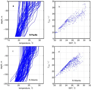
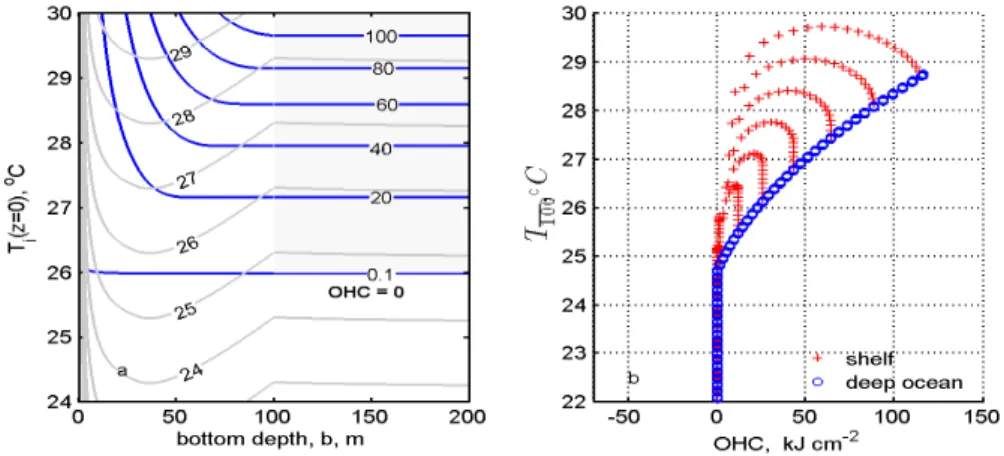
Two open ocean regions are considered here; one is a 10 by 10 degree region of the western subtropical North Pacific centered on 23◦N and 128◦E that was studied by Lin et al. (2008). The available Argo temperature and salinity profiles were acquired for the months July through October of 2007 (297 profiles in total, Fig 6a). This region spawns some of the largest and most intense hurricanes (super typhoons) found anywhere in 10

the world, and it is also a region having pronounced variability of the ocean mesoscale (Qiu, 1999). Eddies having a diameter of several hundred kilometers and sea surface height anomalies of±20 cm are common. These mesoscale eddies are accompanied by a raised or depressed thermocline (Fig. 5) and thus by substantial variations of OHC orT₁₀₀that are not well correlated with sea surface temperature (Fig. 6b and compare 15

Figs. 2 and 3 and Figs. 2 and 4). As noted already, Lin et al. (2008) found that the intensification of the most intense super typhoons is spatially correlated (coincident) with warm eddies (depressed thermocline) that show up as regions of high OHC. These are also regions of very high T₁₀₀ orT_d (Fig. 5 and more below). The second open ocean region considered was the equivalent from the western North Atlantic, 15–30 20

◦

N, and 100–140◦W and for the same months of 2007. These North Atlantic data (and a few profiles from the Caribbean Sea, 313 profiles total) are almost indistinguishable from the North Pacific data, the only difference being fewer points in the range of very large OHC (Fig. 6c and 6d). Within both data sets there are no doubt profiles that were significantly effected by a typhoon or a hurricane. There is no attempt to sort these out, 25

(16)

ap-OSD

6, 909–951, 2009

interaction

J. F. Price

Title Page

Tables Figures

◭ ◮

Back Close

Full Screen / Esc

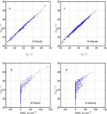
Interactive Discussion proximately equal (Fig. 7a and 7c). This means only thatd=100 m is about the same

on average as is the variabled computed from Eq. (3) for each profile and for a cate-gory 3–4 hurricane. There is some variation of the estimatedd within this sample: d

is as large as 125 m on the most weakly stratified profiles (profile (a) of Fig. 5), and so

T_d is slightly cooler than T₁₀₀ in the range of cool temperatures; d is as small as 85 m 5

on the profiles that are most strongly stratified (profile (b) of Fig. 5), but the resultingT_d

is almost indistinguishable from the fixed depth version,T₁₀₀.

3.1.1 Warm oceans and the high range of OHC

Both of the depth-averaged temperatures are closely related (bijective) with OHC in the high range ofT₁₀₀ , T₁₀₀≥27◦C and OHC, OHC≥75 kJ cm−2 (Fig. 7b, 7d) It is not 10

surprising that an especially warm, thick surface layer will indicate high values of OHC,

T₁₀₀andT_d alike. What is not obvious is that the relationship between high range OHC and highT₁₀₀appears to be very tight and almost identical in the western North Pacific and Western North Atlantic. Thus within a subtropical, summertime map, the contour lines of high T₁₀₀ are parallel with contour lines of high value OHC, and hence the 15

high values ofT₁₀₀ are expected to bear the same qualitative, spatial correlation with hurricane intensification as do high values of OHC (Lin et al., 2008; Shay et al., 2000; Mainelli et al., 2008; and compare Figs. 3 and 4). A depth-averaged temperature, either T₁₀₀ or T_d, thus repeats the most useful, demonstrated property of OHC, viz., high values ofT₁₀₀will identify open ocean regions where the thermal field is especially 20

favorable for hurricane intensification. This was not accommodated after the fact, but follows straightforwardly from the definition of a depth-averaged temperature, Eq. (2), and the empirical relation between high range OHC andT₁₀₀seen in these data (Fig. 7). Indeed, the relation between high-range OHC andT100is so tight that if only warm,

deep ocean conditions were relevant, then there wouldn’t be any practical motive to 25

(17)

OSD

6, 909–951, 2009

interaction

J. F. Price

Title Page

Tables Figures

◭ ◮

Back Close

Full Screen / Esc

Interactive Discussion Sect. 3.2.2, there may be shallow water regions that are equally favorable for hurricane

intensification as assessed by a depth-averaged temperature, and yet that are missed altogether by the high OHC criterion that works well over a warm, deep ocean. Cool, deep ocean regions are also interesting.

3.1.2 Cooler oceans and the low range of OHC

5

OHC andT₁₀₀ are not closely related in the range of low OHC, OHC≤50 kJ cm−2 and low temperatures,T₁₀₀≤26.5◦C (Fig. 7b and 7d). As noted in Sect.1.1, neither is there a statistical correlation between hurricane intensity and OHC within this low range of OHC (Lin et al., 2008; Mainelli et al., 2008). It could be the case that hurricanes are intrinsically not sensitive to low values of OHC so that (an undefined) low sensitivity 10

is swamped by other, uncontrolled factors that appear as noise. However, there is evidence that hurricanes are significantly damped by a sufficiently cool SST (Monaldo et al., 1997; Walker et al., 2005) so that on the face of it, an ocean thermal metric should be expected to have a corresponding range in which hurricane intensity is damped.

While we can not discount the low sensitivity argument, a partial resolution of this 15

issue may be as close at hand as Eq. (1): the loss of the tight relationship between high range OHC and the depth-averaged temperatures results from what is, on second look, a slightly peculiar property built into OHC, i.e., that all ocean temperatures less than the reference temperature 26◦C are counted as zero. For example, if the temperature of a water column was 0◦C, then the estimated OHC would be zero, and if the tempera-20

ture of the water column was 26◦C, then the OHC would again be exactly zero; insofar as OHC is concerned,T=0 and T=26◦C are one and the same. As a consequence, roughly a third of the open ocean temperature profiles considered here (Fig. 7) map into one point in OHC-space, OHC₌0, which might be termed a cool degeneracy. In maps of OHC this appears as regions that are at or near zero and of course horizontally 25

(18)

OSD

6, 909–951, 2009

interaction

J. F. Price

Title Page

Tables Figures

◭ ◮

Back Close

Full Screen / Esc

Interactive Discussion prominent once seasonal cooling has developed in late October; see Goni and

Tri-nanes (2003) and http://www.aoml.noaa.gov/phod/cyclone/data/go.html for examples. In Sect. 1.1 it was noted that the reference temperature of OHC, 26◦C, had a signif-icant empirical basis. But whether there is a corresponding, literal cutoffin hurricane-ocean interaction for SST≤26◦C seems unlikely, if only because the wet bulb temper-5

ature of the hurricane lower atmosphere is usually a few ◦C less than the dry bulb temperature and of course there must be some variation in hurricane air temperatures. What appears to be certain is that OHC defined by Eq. (1) will have poor (or no) res-olution in regions where the upper ocean temperature is comparable to or less than 26◦C and hence OHC could not be expected to provide a nuanced account of the 10

possible damping e_ffect of still lower SST. This limitation of OHC is not shared by a depth-averaged temperature.

3.2 The coastal ocean

OHC and the depth-averaged temperatures can be quite different when evaluated over shallow water regions. The consequence for forecasts of hurricane-ocean interaction 15

may be more or less significant depending upon the extent of the shallow water area affected in relation to a hurricane track. However, there can be little doubt that the limit of vanishing water depth should be treated in a physically plausible way by any hurricane forecasting scheme since it occurs in conjunction with hurricane land fall.

To illustrate the effects of bottom depth alone, OHC andT_d were evaluated over an 20

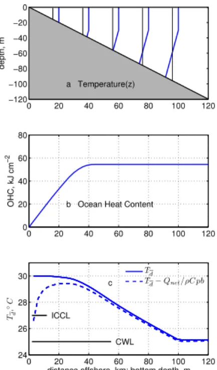
idealized continental shelf that was constructed along the lines of the West Florida Con-tinental Shelf (Fig. 8a). The bottom slope was taken to be∂b/∂x=10−3and constant, withbthe bottom depth, and x the across-shelf coordinate. The hydrography of con-tinental shelves can vary a great deal from region to region (Allen et al., 1983) with important consequences for what follows. Given that the goal here is to illustrate bot-25

(19)

OSD

6, 909–951, 2009

interaction

J. F. Price

Title Page

Tables Figures

◭ ◮

Back Close

Full Screen / Esc

Interactive Discussion The temperature profile Ti(z) was taken from the West Florida Shelf in summer (Hu

and Muller-Karger, 2007) and had a warm and quasi-uniform surface layer about 25 m thick, and a comparatively large vertical gradient of temperature, 0.15◦C m−1, within the seasonal thermocline. This kind of shallow, strongly stable seasonal thermocline is typical of subtropical shelf regions that are not directly influenced by deep ocean 5

currents, e.g., the South Atlantic Bight and the Middle Atlantic Bight (Schofield et al., 2008), if not impacted by Gulf Stream-derived eddies, or the northern Gulf of Mexico, aside from Loop Current eddies. The metrics OHC andT_d were then sampled along a transect across the shelf (Figs. 8b and 8c).

3.2.1 Coastal ocean OHC

10

To evaluate OHC over shallow waters in which the bottom temperature exceeds 26◦C, the lower limit of integration was presumed to be the bottom depth, b. Given this specific shelf and hydrography, the estimated OHC begins to decrease as the bottom depth becomes less than the depth of the 26◦C isotherm, which is about 50 m in the temperature profile presumed here (Fig. 8b). Assuming a consistent deep-ocean and 15

coastal-ocean interpretation of OHC, i.e., that regions having OHC≤50 kJ cm−2are not favorable for hurricane intensification (or at least less so than high OHC regions), then a shallow continental shelf would appear to be an unfavorable environment for hurricane intensification. We are going to suggest below that this may not be the case.

This consideration of a coastal ocean shows that OHC can vanish in two important, 20

realizable limits: 1) over the deep ocean as T→26◦C from above, and discussed in

the previous section, and, 2) over a coastal ocean as b→0 and regardless of the temperature. If the underlying issue for hurricane-ocean interaction is SST rather than OHCper se, as we have argued it must be in P1 of Sect. 2, then it appears that OHC suffers from a second kind of degeneracy in shallow water in that very low values of 25

(20)

OSD

6, 909–951, 2009

interaction

J. F. Price

Title Page

Tables Figures

◭ ◮

Back Close

Full Screen / Esc

Interactive Discussion the same consequence for hurricane-ocean interaction as do low values over the deep

ocean. The combined e_ffect of this cool and shallow water degeneracy is likely to be a part of the reason that OHC does not show a correlation with hurricane intensification in the low range of OHC (Mainelli et al., 2008).

3.2.2 Coastal oceanT

d 5

A coastal warm layer: given the shelf topography and stratification presumed here, the depth-averaged temperatureT_d increases as the bottom depth becomes less than

d_{d o}=85 m, the depth of mixing over the deep ocean given this rather stable stratifi-cation. The increase of T_d shoreward of the 85 m isobath (Fig. 8c) follows from the increase of bottom temperature with decreasing bottom depth; as the bottom temper-ature increases there is less cold water available to be mixed upwards. This can be expected over a shelf on which the seasonal thermocline intersects the bottom, i.e., over shelves that are either upwelling neutral or negative. The result is that the across-shelf temperature profileT(x) exhibits what might be termed a Coastal Warm boundary Layer (CWL), whose half-width may be estimated roughly as

WCWL≈

1 2dd o/

∂b

∂x, (4)

and in this case,WCWL=55 km.

An inner-coastal cool layer: heat loss to the hurricane must become a significant process for sea surface cooling where the water is shallow enough (Shen and Ginis, 2003). To account approximately for this hurricane-ocean heat exchange, the depth-averaged temperatureT_d can be perturbed by subtracting a typical net hurricane-ocean heat flux,Qnet, from the water column. Qnetis estimated roughly as the average heat

loss from the ocean to a hurricane, 1000 W m−2, times a typical hurricane residence time, 12 h (Cione and Uhlhorn, 2003; Chen et al., 2007), and soQnet≈4×10

7

J m−2, or in the non-SI units often used for OHC,Qnet≈4 kJ cm

−2

(21)

OSD

6, 909–951, 2009

interaction

J. F. Price

Title Page

Tables Figures

◭ ◮

Back Close

Full Screen / Esc

Interactive Discussion temperature is then,

T_d−Q_net/ρ_oC_pb, (5) whereb is the water depth, shown as the dashed line of Fig. 8c. The resulting Inner-Coastal Cool boundary Layer (ICCL), follows the qualitative expectations of OHC in the sense that the cooling is inversely related to water depth,b. The width of this cool layer may be estimated roughly as the region where the temperature is decreased by ∆T=1◦C or more,

ICCL≈

Qnet

ρ_oC_p∆T/ ∂b

∂x, (6)

and in this case,WICCL=12 km.

Thus the post-hurricane coastal ocean sea surface temperature computed by the

T_d model may show two boundary layers when compared to the outlying and otherwise similar deep ocean – a coastal warm layer (CWL, and warm compared to the outlying deep ocean) in which the characteristic process is a reduced heat flux associated with vertical mixing, and an inner-coastal cool layer (cool compared to the warm layer), in which hurricane ocean heat exchange is important. This ICCL follows the expectations implicit to OHC, and a comparison of the amplitude and width of the ICCL and the CWL gives a visual impression of the relative importance of vertical mixing and hurricane-ocean heat exchange, insofar as the SST over a continental shelf is concerned. Given the upwelling neutral shelf considered here, the outer warm layer is considerably wider than the inner cool layer. For typical bottom slopes and heat loss values,

WCWL

WICCL

= dd o/2

Q_net/ρ_oC_p∆T ≈4. (7)

(22)

OSD

6, 909–951, 2009

interaction

J. F. Price

Title Page

Tables Figures

◭ ◮

Back Close

Full Screen / Esc

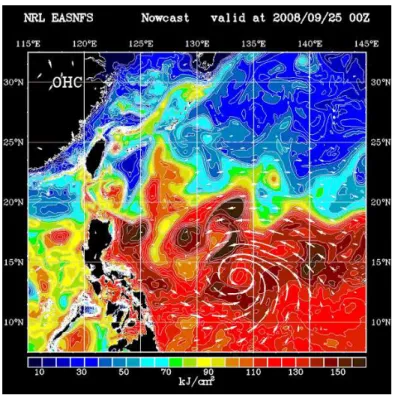
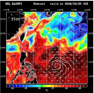
Interactive Discussion These are depicted as regions of generally low OHC,≤40 kJ cm−2, despite having fairly

high SST, simply because they are shallow. In contrast, the estimated depth-averaged temperature (Fig. 4 isT₁₀₀ which has the same relation to bottom depth as does Td)

indicates that these shelf regions are likely to remain fairly warm during a hurricane passage by virtue of the CWL phenomenon. Hence these shelf regions appear to be 5

somewhat favorable for hurricane intensification, as seen in a depth-averaged temper-ature T₁₀₀≥27◦C. Some of the effected shelf regions are as wide as several hundred kilometers and likely to be of significance for hurricane-ocean interaction, or at least for our prediction of hurricane-ocean interaction. Other shelf regions appear nearly the same when diagnosed with OHC orT₁₀₀, notably east of the Phillipines, where the con-10

tinental shelf is quite narrow. To summarize – on the results presented here, at least some coastal oceans – those having broad, shallow continental shelves and hydrogra-phy that is upwelling neutral or negative – would appear to be favorable environments for hurricane intensification (Fig. 9), a result that could not have been anticipated from OHC.

15

3.2.3 Coastal ocean observations

As hurricanes cross a continental shelf they are also very likely to be making land fall, which is usually expected to cause a rapid and significant decrease of hurricane in-tensity (but see McTaggart-Cowen et al., 2007, who note that this is not necessarily the case if the land surface is flat, warm and wet, e.g., South Florida). However, our 20

concern here is exclusively with the ocean thermal field, and some evidence is that shallow water environments may indeed be favorable for hurricane intensification. That is, hurricane-induced sea surface cooling has been observed to be reduced over shal-low water regions compared to the cooling over outlying, deep water regions. Hazel-worth (1968) analyzed the time series data from weather ships for hurricane passages, 25

(23)

OSD

6, 909–951, 2009

interaction

J. F. Price

Title Page

Tables Figures

◭ ◮

Back Close

Full Screen / Esc

Interactive Discussion phenomenon has been observed on the West Florida Continental Shelf by Hu and

Muller-Karger (2003). The latter two studies inferred that the principal cause of the reduced sea surface cooling over shallow water was the absence of cool water at depths that could be mixed into the surface layer, just as happens here with the depth-averaged temperature. Emanuel (1999) noted the relevance of this shallow water effect 5

in the context of hurricane-ocean interaction.3

3.3 Salt-stratified water column

In the event that salinity makes an important contribution to the upper ocean density stratification, thenT_d can, in principle, differ from both OHC and T₁₀₀ which acknowl-edge temperature only. Important salinity effects may arise where there is a compara-10

tively fresh ocean surface layer, which often occurs in a coastal ocean, and especially down-coast from the estuary of a major river (Price, 1981; Bingham, 2007). There are also open ocean regions in which salinity makes an appreciable contribution to the static stability of the upper ocean, e.g., the barrier layer of the western tropical Pacific and parts of the Indian Ocean (McPhaden et al., 2009).

15

If the net salinity anomaly (thickness times salinity anomaly in the initial state) is as large as about 20 m, then the fresh layer will inhibit vertical mixing significantly. The e_ffect upon the sea surface temperature will depend upon whether the fresh layer is

3

During the summer of 2005 there were a number of intense hurricanes that crossed over the Gulf of Mexico, including Katrina (2005), which passed over the Louisiana shelf, and Wilma (2005), which passed over Florida Bay and the southern end of the West Florida

shelf. SST imagery of these significant events provides some additional qualitative

evi-dence of a coastal warm layer and sometimes a hint of an inner-coastal cool layer, though

not always distinct from land effects; see the collection of GOES-12 SST images in http:

(24)

OSD

6, 909–951, 2009

interaction

J. F. Price

Title Page

Tables Figures

◭ ◮

Back Close

Full Screen / Esc

Interactive Discussion warmer or cooler than the water below. If the former, then salinity stratification will

act to reduce the depth of vertical mixing and thus sea surface cooling. If the latter, then vertical mixing will act to increase the surface temperature (see the Nordic Sea example of Saetra et al., 2003), a possibility missing altogether from OHC, which omits any reference to salinity (or density). This anomalous surface warming e_ffect of vertical 5

mixing would be present in T₁₀₀, but in general, a salinity effect upon static stability requires an explicit treatment of density, e.g., by means ofT_d or something more com-prehensive.

4 In closing

4.1 Summary

10

The standard metric of the ocean thermal field within hurricane-ocean interaction is a depth-integrated ocean temperature, upper Ocean Heat Content or OHC. OHC has been shown to provide valuable forecast guidance in warm, deep ocean conditions (Lin et al., 2008; Mainelli et al., 2008) but the argument made here is that a depth-averaged temperature,T₁₀₀ orT_d, may be more appropriate over a much wider range of condi-15

tions. The argument was made on two premises: P1, that SST and especially SST under a hurricane is the directly relevant ocean variable, and P2, the observation that cooling is due mainly to vertical mixing rather than to hurricane-ocean heat exchange. Two hypotheses follow: H1, a depth-averaged ocean temperature is the direct proxy (or metric) for SST under a hurricane, and H2, a depth-averaged temperature is a more 20

robust metric of hurricane-ocean interaction than is OHC.

The majority of hurricanes and typhoons form over the deep, open ocean in late summer when sea surface temperature is warmest. In that circumstance, OHC and

T₁₀₀ orT_d will provide essentially the same forecast guidance, i.e., that an ocean re-gion having a warm (T≥26◦C) thick surface layer will be a favorable environment for

(25)

OSD

6, 909–951, 2009

interaction

J. F. Price

Title Page

Tables Figures

◭ ◮

Back Close

Full Screen / Esc

Interactive Discussion hurricane intensification. This could be taken as a warrant for OHC – that a high OHC

region resists cooling due to hurricane-ocean heat exchange (which we have sug-gested is not plausible, Sect. 2.1), or equally, evidence in favor ofT₁₀₀ orT_d – that a thick warm surface layer resists the cooling effect of vertical mixing. This latter interpre-tation is in common with most recent studies (Lin et al., 2008; McTaggart-Cowen et al., 5

2007; Mainelli et al., 2008) and is the interpretation espoused and implemented here in the form of an ocean metric. Admittedly, if only warm and deep ocean conditions were relevant, then this distinction would be of little or no practical importance (Fig. 9). 4

But there are at least three other realizable circumstances in which the mechanism becomes crucially important in as much as OHC and depth-averaged temperature will 10

give quite di_fferent forecast guidance (1). Cool, open ocean waters. Hurricanes tend to form over warm (SST≥26◦C) regions, but may later move over much lower SSTs during their life cycle (a striking example is shown by Monaldo et al., 1997). The cool

4

The seasonal cycle of cooling on warm subtropical continental shelves serves as an inter-esting counterpoint to the hurricane-ocean interaction phenomenon of interest here. Around the Gulf of Mexico, the cooling phase of the seasonal cycle begins in earnest with the first cold air outbreak (see the satellite imagery noted above and the cold air outbreak beginning in mid-October, 2005 following the passage of Hurricane Wilma, 2005). Where a hurricane can

be characterized by very strong winds and a rather small air-sea temperature difference, cold

air outbreaks over the Gulf of Mexico are the complement in the sense that they have moderate

wind speeds but very cold and dry air that sets up a very large air-sea temperature difference

(26)

OSD

6, 909–951, 2009

interaction

J. F. Price

Title Page

Tables Figures

◭ ◮

Back Close

Full Screen / Esc

Interactive Discussion degeneracy built in to OHC effectively restricts its application to warm ocean conditions.

The depth-averaged temperatures do not have this property, and an analysis of T₁₀₀

orT_d could, in principle, allow for a forecast (or explain, in hindcast) a damping effect of cool sea surface temperatures upon hurricane intensity (though it remains to define what that may be) (2). Salt-stratified waters. While temperature is a sufficient proxy 5

for density and static stability in most conditions, salinity can have a significant and sometimes decisive effect on static stability in special locations, for example within or near estuaries. OHC andT₁₀₀are silent on salinity effects, which can be accounted by a model that estimates vertical mixing from static stability,T_d, provided that salinity is known (3). Shallow waters. OHC and the depth-averaged temperatures can be quite 10

di_fferent when evaluated over shallow, continental shelf regions. OHC will generally indicate that shallow regions (shallow compared to the depth of the 26◦C isotherm) are an unfavorable environment for hurricane intensification, whileT₁₀₀orT_d may indicate the opposite, that shallow regions (shallow compared to the depth of vertical mixing in the deep ocean, d_{d o}) can be favorable for hurricane intensification compared to 15

an otherwise similar deep ocean (Fig. 9). To the point – this study indicates that, land e_ffects aside, a shallow, warm continental shelf may be as favorable for hurricane intensification as is a deep, open ocean, warm regime, e.g., the Loop Current or warm eddies of the subtropical gyre interior (compare the depth averaged-profiles of Fig. 5a and 5c).

20

4.2 Remarks on the coastal ocean

SST and distance offshore are at once the most readily observed property of the coastal ocean and are the property of immediate interest for hurricane-ocean interac-tion and forecasting. It is important to appreciate that the specific relainterac-tionship between SST and distance offshore shown in Fig. 8c is not universal because the hydrography 25

(27)

OSD

6, 909–951, 2009

interaction

J. F. Price

Title Page

Tables Figures

◭ ◮

Back Close

Full Screen / Esc

Interactive Discussion the depth and (at least) the cross-shelf coordinate,x, so thatT=T(x, z). In shelf regions

that are upwelling positive, e.g., Campeche Bank or the Louisiana-Texas shelf in late summer (Walker, 2005), the thermocline will be lifted toward the coast (∂T_∂x≥0 for the configuration of Fig. 8a) and cool water may be present very close to shore and very close to the sea surface. Preliminary calculations (not shown here) suggest that even 5

fairly modest upwelling can bring enough cool water onto the inner shelf to eliminate or reverse the OCWL that is expected over upwelling neutral or negative shelf regions. On some shelves, e.g., the Middle Atlantic Bight, the early summer thermocline may be thin enough, O(30 m) (Schofield et al., 2008) that the width of the coastal warm layer may be no more than a few kilometers, and so probably negligible. Given the 10

great range and temporal variability of coastal ocean hydrography, a key requirement for forecasting hurricane-ocean interaction over shelf regions will be to observe and to model the ocean stratification in more or less real time.

The present treatment of the coastal ocean response to a hurricane (Sect. 3.2.2) was simplified to the point that T_d could be characterized as a null model: the esti-15

mated (deep ocean) vertical mixing was simply stopped if it reached the ocean bottom. That must happen, of course, but so may a great deal else that was outside the scope of the present treatment. For example, rotary inertial motions, which dominate the ver-tical shear of the open ocean wind-driven current, must be inhibited near coast lines. At a minimum, there must occur transient up- and down-welling that was not accounted 20

for in the local version ofT_d presented here. Surface gravity waves generated by an approaching hurricane can be very energetic, and may cause intense vertical mixing within a thick bottom boundary layer, even before the direct effect of the hurricane wind stress reaches the bottom (Glenn et al., 2008). Finally, the pre-hurricane thermal and salinity fields around continental shelves will often vary in three dimensions, with 25

(28)

OSD

6, 909–951, 2009

interaction

J. F. Price

Title Page

Tables Figures

◭ ◮

Back Close

Full Screen / Esc

Interactive Discussion space for hurricane-coastal ocean interaction is very extensive and well worth

addi-tional study and synthesis. We certainly need to understand which map – OHC in Fig. 3 orT₁₀₀ in Fig. 4 – gives the better account of hurricane-ocean interaction over continental shelves, and over cool, open ocean regions.

5 A look ahead

5

Forecasting of hurricanes or any natural phenomenon is a pragmatic endeavor. Insight from models and observations can help to point the way to new hypotheses or methods, but forecasting success can only be told from actual practice (Lin et al., 2008; Mainelli et al., 2008) which was not attempted here. The best result of this discussion would be to stimulate a fresh look at hurricane-ocean interaction, and specifically, to encourage 10

further testing of ocean metrics drawn from an expanded hypothesis-space. Just two examples: A revised OHC: the conservation error of OHC (footnote 1 of Sect. 1), along with the cool degeneracy noted in Sect. 3.1.2 could be remedied for most hurricane analysis or forecasting purposes simply by choosing a reference temperature that is below the depth of vertical mixing and the lower limit of relevant SSTs, e.g., 22◦C. This 15

variant of OHC will have improved conservation and statistical properties over a wider range of conditions than does the usual form, Eq. (1), but there is still no guarantee that heat content will be the most relevant physical quantity for hurricane-ocean interac-tion over shallow continental shelves (Sect. 3.2) and especially those that are to some degree salt-stratified (Sect. 3.3). A derivative ofT_d: the depth-averaged temperatures 20

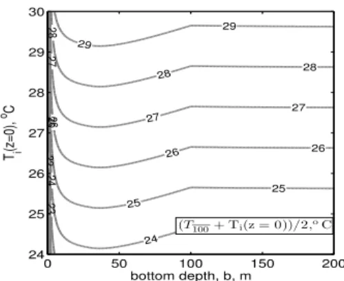
estimated here were intended to be the minimum of SST expected in a hurricane wake. An important question beyond the present scope is whether hurricane-ocean interac-tion could be better represented by something other than this minimum SST, e.g., an average of the observed pre-hurricane SST andT_d would be a better approximation to the SST under the maximum winds of a hurricane (Cione and Uhlhorn, 2003; Fig. 10). 25

(29)

OSD

6, 909–951, 2009

interaction

J. F. Price

Title Page

Tables Figures

◭ ◮

Back Close

Full Screen / Esc

Interactive Discussion wind stress amplitude in the mixing model (Eq. 3),τ=0.5 Pa, would be appropriate.

Ex-plicit treatment of slowly moving storms would require development of the lowUh limit

to account for upwelling and, in shallow water, heat loss to the hurricane.

Discovering the optimum ocean metric is not likely to come easily; OHC and depth-averaged temperatures are well-correlated in some important circumstances and, in 5

any event, the ocean thermal field is just one of several factors that make up the com-plex environment of a hurricane. A thorough exploration and sensitive test of ocean metrics will require a large suite of case studies that span the full range of ocean con-ditions that are relevant for hurricane-ocean interaction. No doubt such a study could be aided considerably by guidance from the best possible air and sea coupled models 10

that include a coastal ocean.

Acknowledgements. This research was supported by the US Office of Naval Research through

the project Impact of Typhoons on the Western North Pacific (ITOP). Thanks to T. Sanford of the Applied Physics Laboratory, University of Washington for the EM-APEX data of Fig. 1 and for valuable comments on a draft manuscript. Thanks to J. J. Park and Y.-O. Kwon of the

15

Woods Hole Oceanographic Institution for the quality-controlled Argo data sets and to ITOP colleagues Dong-Shan Ko of the Naval Research Laboratory, S. Jayne of the Woods Hole Oceanographic Institution, E. D’Asaro of the Applied Physics Laboratory, University of Wash-ington, I.-I. Lin of Taiwan National University and S. Chen of the University of Miami for valuable discussions of this research. T. Farrar and B. Warren of Woods Hole Oceanographic Institution

20

(30)

OSD

6, 909–951, 2009

interaction

J. F. Price

Title Page

Tables Figures

◭ ◮

Back Close

Full Screen / Esc

References

Allen, J. S., Beardsley, R. C., Blanton, J. O. , et al.: Physical oceanography of continental shelves, Rev. Geophys., 21(5), 1149–1181, 1983.

Bender, M. A., Ginis, I., and Kurihara, Y.: Numerical simulations of tropical cyclone-ocean inter-action with a high resolution coupled model, J. Geophys. Res.-Atmos., 98, 23,245–23,263,

5

1993.

Bender, M., Ginis, I., Tuleya, R., Thomas, B., Marchok, T.: The operational GFDL coupled hurricaneocean prediction system and a summary of its performance, Mon. Weather Rev., 135, 3965–3989, 2007.

Bingham, F. M.: Physical response of the coastal ocean to Hurricane Isabel near landfall,

10

Ocean Sci., 3, 159–171, 2007, http://www.ocean-sci.net/3/159/2007/.

Black, P. G., D’Asaro, E., Drennan, W. M., French, J. R., Sanford, T. B., Terrill, E. J. , Niiler, P. P., Walsh, E. J., and Zhang, J.: Air-sea exchange in hurricanes: Synthesis of observations from the Coupled Boundary Layer Air-Sea Transfer Experiment, B. Am. Meteorol. Soc., 88,

15

357–374, 2007.

Chen, S. S., Price, J. F., Zhao, W., Donelan, M. A., and Walsh, E. J.: The CBLAST-Hurricane program and the next-generation fully coupled atmosphere-wave-ocean models for hurricane research and prediction, B. Am. Meteorol. Soc., 88, 311–317, 2007.

Chu, P. C., Veneziano, J. M., Fan, C., Carron, M. J., and Liu, W. T.: Response of the South China

20

Sea to Tropical Cyclone Ernie 1996, J. Geophys. Res., 105(C6), 13,991–14,009, 2000. Cione, J. J. and Uhlhorn, E. W.: Sea surface temperature variability in hurricanes: Implications

with respect to intensity change, Mon. Weather Rev., 131, 1783–1796, 2003.

Cornillon, P., Stramma, L., and Price, J. F.: Satellite observations of sea surface cooling during hurricane Gloria, Nature, 326, 373–375, 1987.

25

D’Asaro, E. A., Sanford, T. B., Niiler, P. P., and Terrill, E. J.: Cold wake of Hurricane Frances, 34, L15609, doi:10.1029/2007GRL030160, 2007.

DeMaria, M., Mainelli, M., Shay, L. K., Knapf, J. A., Kaplan, J.: Further improvements to the Statistical Hurricane Intensity Prediction Scheme (SHIPS), Weather. Forecast., 20, 531–543, 2005.

30