Parameterizing Spatial Models of Infectious Disease Transmission that Incorporate Infection Time Uncertainty Using Sampling-Based Likelihood Approximations.

Parameterizing Spatial Models of Infectious

Disease Transmission that Incorporate

Infection Time Uncertainty Using

Sampling-Based Likelihood Approximations

Rajat Malik1*, Rob Deardon1,2,3*, Grace P. S. Kwong3*

1Department of Mathematics & Statistics, University of Guelph, Guelph, Ontario, Canada,2Faculty of Veterinary Medicine, University of Calgary, Calgary, Alberta, Canada,3Department of Mathematics & Statistics, University of Calgary, Calgary, Alberta, Canada

*rmalik@uoguelph.ca(RM);robert.deardon@ucalgary.ca(RD);grace.kwong@ucalgary.ca(GPSK)

Abstract

A class of discrete-time models of infectious disease spread, referred to as individual-level models (ILMs), are typically fitted in a Bayesian Markov chain Monte Carlo (MCMC) frame-work. These models quantify probabilistic outcomes regarding the risk of infection of sus-ceptible individuals due to various susceptibility and transmissibility factors, including their spatial distance from infectious individuals. The infectious pressure from infected individu-als exerted on susceptible individuindividu-als is intrinsic to these ILMs. Unfortunately, quantifying this infectious pressure for data sets containing many individuals can be computationally burdensome, leading to a time-consuming likelihood calculation and, thus, computationally prohibitive MCMC-based analysis. This problem worsens when using data augmentation to allow for uncertainty in infection times. In this paper, we develop sampling methods that can be used to calculate a fast, approximate likelihood when fitting such disease models. A sim-ple random sampling approach is initially considered followed by various spatially-stratified schemes. We test and compare the performance of our methods with both simulated data and data from the 2001 foot-and-mouth disease (FMD) epidemic in the U.K. Our results indi-cate that substantial computation savings can be obtained—albeit, of course, with some information loss—suggesting that such techniques may be of use in the analysis of very large epidemic data sets.

Introduction

Modeling the spread of infectious diseases is a research area of great importance to public health and agriculture. Particularly, studies involving data-driven spatial models have recently been used in a number of applications. Work by [1], for example, illustrate the importance of incorporating spatial and temporal data in the mathematical modeling of infectious diseases. Studies have also investigated factors that influence disease persistence/extinction such as

OPEN ACCESS

Citation:Malik R, Deardon R, Kwong GPS (2016) Parameterizing Spatial Models of Infectious Disease Transmission that Incorporate Infection Time Uncertainty Using Sampling-Based Likelihood Approximations. PLoS ONE 11(1): e0146253. doi:10.1371/journal.pone.0146253

Editor:Gui-Quan Sun, Shanxi University, CHINA

Received:July 9, 2015

Accepted:December 15, 2015

Published:January 5, 2016

Copyright:© 2016 Malik et al. This is an open access article distributed under the terms of the Creative Commons Attribution License, which permits unrestricted use, distribution, and reproduction in any medium, provided the original author and source are credited.

Data Availability Statement:The data we utilized, called the 2001 UK foot and mouth disease farm-level data set, was obtained from the United Kingdom Government Department of Environment, Food and Rural Affairs (DEFRA), and were given permission by them to use the data for our paper. We do not, however, have permission to redistribute the data. If any readers wish to obtain the data, they may contact Dr. Deardon or DEFRA directly atdefra.

helpline@defra.gsi.gov.uk.

infection rate (e.g., [2]). In addition, disease control policies and vaccination policies can be better developed as a result of the understanding of the spread of infectious disease gained from using such models [3]. The increase in computational power over the last several years and the availability of spatio-temporal data have been key factors driving growth in this area of statistics [4].

Significant computational prowess is required for models utilizing large-scale spatial data, such as recent studies performed on the 2001 foot-and-mouth disease (FMD) epidemic in the U.K. (e.g., [5–8]). These can all be considered examples of modeling infectious disease dynamics at the individual-level, although the individuals of concern may vary between stud-ies (e.g., plants, humans, farms, etc.). [8] describe a framework of discrete-time individual-level models (ILMs) that are capable of modeling the spread of infectious diseases in such dis-ease systems. These models can incorporate various heterogeneities within a population; for example, [9] consider the spread of human influenza allowing for vaccination status, age, and the disease status of fellow household occupants in the model. Although ILMs are flexible and intuitive, inference for these and other similar models, especially when dealing with large data sets, can be computationally prohibitive. In fact, even for moderately sized populations, obtaining meaningful results can require running these models for a considerable amount of time.

For such models, parameter estimation is typically carried out in a Bayesian framework via Markov chain Monte Carlo (MCMC) methods (e.g., [10]), wherein the likelihood function (a primary source of the computational problem) is calculated numerous times. An obvious way to reduce the extent of this problem would be to make a simplifying assumption, such as homogeneous mixing (e.g., [11]). However, by allowing for heterogeneity within the popula-tion, we hope to draw more sound inferences.

Numerous studies have focused on speeding up the likelihood calculation to reduce the time required to carry out parameter estimation in such models. For example, [8] introduce an approach using a Taylor series expansion of the non-linear spatial infection kernel, allowing for the decomposition of a substantial part of the likelihood function into a small parameter-dependent part and a larger data-parameter-dependent part. [12] expand on this by exploring the use of a piecewise linear kernel to carry out the linearization. In both cases, time-saving ensues from the fact that the data-intensive component of the likelihood does not require re-calculation at each step of the MCMC algorithm. However, the resulting model is an approximation of the true model we might actually want to fit. These approaches are also limited to situations where infection event histories of individuals are assumed known.

[13] explore several variations of a random-walk Metropolis algorithm to achieve computa-tional efficiency in the context of infectious disease modeling. Their approach involves pre-cal-culating and storing quantities that are used repeatedly (something vital to the approaches of [8] and [12]), performing calculations in parallel, and refining the calculation of the likelihood ratio in the Metropolis-Hastings MCMC algorithm.

Other approaches to decreasing computation time in the context of fitting infectious disease models to data—in these cases, homogeneous-mixing models—are based around so-called approximate Bayesian computations, as explored in [14] and [15], and pseudo-marginal approaches, as discussed by [16]. In such approaches, explicit likelihood calculation is completely avoided. An alternative approach is given by [17], not within the context of infer-ence for infectious disease transmission models, but for mixture models. They explore methods basing inference on carefully selected subsamples of data, constructed to provide the most rele-vant information to the parameters of interest.

In this paper, we consider an approach similar in nature to that of [17] that replaces the like-lihood calculation with a faster likelike-lihood approximation based upon data sampling. We also Engineering Research Council of Canada (NSERC).

Computer equipment was provided by the Canada Foundation for Innovation via the Leading Edge Fund grant,“Centre for Public Health and Zoonoses (CPHAZ).”

include infection time uncertainty in our modeling via a data augmented Bayesian analysis. The method works by selecting samples from the infected set of individuals at every discrete time point when calculating the infection rate for susceptible individuals, thereby avoiding the need to use the entire infectious set. We show how the resulting approximated likelihood func-tion-based analysis can require significantly less time to carry out and compare the approxi-mate posterior inference to the full Bayesian analysis. Whereas the aforementioned

approximate methods of [8] and [12] for parameterizing ILMs cannot be used in a data aug-mented framework in which infection times are considered unknown, we show how our approach, with careful algorithm development, can allow such uncertainty in the analysis. This is of obvious importance in infectious disease systems because infection event times are very rarely observed with any certainty in practice [18]. We begin by considering a simple random sampling (SRS) approach, followed by a series of spatially-stratified sampling schemes. As a proof of concept, we test our methodology through the use of both simulated data and a rela-tively small subset of the 2001 UK FMD epidemic data. Note that we consider infectious dis-ease models in a susceptible-infectious-removed (SIR) framework, although extension of the methods to other frameworks (e.g.,SEIR) would be relatively straight forward.

Our paper is structured as follows. TheMethodologysection summarizes the general ILM framework of [8], the specific models used in this paper, and the MCMC algorithm used to carry out a full Bayesian MCMC analysis. Our algorithms are presented in theSampling-Based Likelihood Approximationssection. TheEpidemic Datasection describes the data used to test our methods and theResultssection presents our findings. TheDiscussionsection concludes this paper and presents possible avenues of future work.

Methodology

General Model

We utilize the modeling framework of [8], which defines a class of flexible discrete-time disease transmission models that include covariate information at the individual level. With a finite population of a total ofnindividuals (each individual represented asi= 1,. . ._{,n), we observe}

epidemic data at discrete time points,t= 1,. . ._,t

max, wheretmaxis the last observation time.

Under a susceptible-infectious-removedðSI RÞframework, each individualiis in only one of these three states at any given timet. Ifi2S_t, theniis susceptible to the disease and has not yet contracted it at timet; ifi2I_t, thenihas contracted the disease and can now infect others at timet; and ifi2R, thenihas been removed from the population at timet; e.g., due to recov-ery combined with acquiring immunity. Once an individual is in thisfinal state, they cannot become infected again or transmit the disease to others. Over the course of the epidemic, indi-viduals move through the three states in the orderS!I!R.

As described by [8], the general ILM calculates the probability a susceptible individualiwill become infectious to the disease at timet, and this is given by

PitðθÞ ¼1 exp OSðiÞ X

j2It

O_TðjÞkði;jÞ

( )

ði;tÞ

" #

; ð1Þ

whereO_{S(i) is a susceptibility function that includes risk factors for individualicontracting the}

disease;O_{T(j) is a transmissibility function describing risk factors for individualjtransmitting}

Spatial ILM

In this section, we present a simplified version of the general ILM such thatO_{S(i) =α,}O_{T(j) =}

1, andkði;jÞ ¼db

ij . Here,dijrepresents the Euclidean distance between susceptibleiand

infec-tiousjandβrepresents the power law rate of decay. We also set the sparks term,(i,t) = 0. We refer to this model as the Spatial ILM. Under this model, the probability of infection for suscep-tibleiat timetis given by

PitðθÞ ¼1exp a X

j2It

db ij " #

; a>0_;b>0_{: ð2Þ}

FMD-ILM

We also modify the general ILM in order to model data from the 2001 U.K. FMD epidemic. Using a simplified version of the model found in [8] and by modeling at the farm-level, we can determine the probability that susceptible farmiis infected at timetusing

PitðyÞ ¼1exp asNisþacNic X

j2It

sNjsþcNjc

db ij

!

" #

;

a_c>0_;

s>0; c>0;b>0; >0;

ð3Þ

whereα_sandα_care susceptibility parameters andϕsandϕcare transmissibility parameters, for

sheep and cattle, respectively. The termsNs xandN

c

xrepresent the number of sheep and cattle

on farmx, respectively. To avoid identifiability issues, we setαs= 1 × 10−7, which is an arbitrary

constant reference level and is not estimated. Once again, the power-law kernel,kði;jÞ ¼dijb,

is used withdijbeing the Euclidean distance between farms. The sparks terms is set as a

con-stant such that(i,t) =, which represents a constant infectious pressure from outside the study area. We refer to Model 3 as our FMD-ILM.

Bayesian Computation

Our parameter estimation is here carried out under a Bayesian framework. Assuming known infection and removal times, the likelihood function for ILMs is the product of all infection and non-infection events over the entire observed epidemic period (t= 1,. . ._,t

max), and is given by

pðx_jθ_{Þ ¼} Y

t_max

t¼1 Y

i2Stþ1

1_P

itðθÞ

ð Þ Y

i2Itþ1nIt

PitðθÞ

" #

; ð4Þ

wherexis the observed epidemic data set (including the infection times),S_tþ1is the set of all

susceptible individuals at timet+ 1, andI_tþ1nI_tis the set of newly infectious individuals at

timet+ 1. Using our likelihood function and by placing a prior,π(θ_{), on our parameter set,}θ_, we can obtain the posterior distribution,π(θ_{|x), up to a constant of proportionality. To explore} the posterior distribution, we can use the random-walk Metropolis Hastings (RWMH) algo-rithm [19–21].

Bayesian data augmentation, treating the infection times as unknown nuisance parameters (see also sectionsMCMC AlgorithmandData Augmentation). We determine the infection time indirectly by inferring the incubation period (the time between infection and disease reporting/ diagnosis/observation) of each individual. Given the aforementioned assumption that removal times are known, the incubation period thus defines the infection time for each individual. The incubation period, plus a further delay until removal (e.g., through quarantine or animal cull-ing), thus define the infectious period.

We denote the unknown incubation periodsZ_{¼ ð}Z1;Z2;. . .;Z_vÞ, wherevis the number

of infected individuals in [1,tmax], and assumeZc

i:i:d

DExpðl_zÞ(discretized exponential distri-bution), where the rate parameter,λz, is also to be estimated. We augment the model parameter

set to includeZ_{. Under the spatial ILM, our parameter vector is thus}θþ_{¼ f}a;b;l_z;Z_{g; and} under the FMD-ILM, the parameter set isθþ_{¼ fa}

c; s; c;b; ;lz;Zg.

In general, we define an augmented parameter set,θþ_{¼ ð}θ_;Z_{Þ, and assuming} indepen-dence betweenθ_andZ_{derive the posterior distribution up to proportionality as}

pðθþ_jx_{Þ / pðxjθ}þ

Þpðθþ_Þ

¼ pðx_{jθ;ZÞpðθÞpðZÞ}

¼ pðx_;Z_jθ_Þpðθ_Þ;

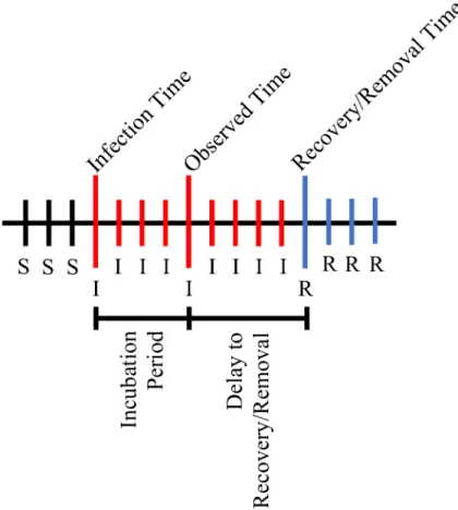
ð5Þ Fig 1. Average infectious period under the simulation study.Illustration of the average infectious period under the simulation study. The average incubation period is 3 days, and the average delay to disease recovery and removal from the population is 4 days. The‘S’symbol indicates the individual is susceptible to the disease at that time point and the‘R’symbol indicates the individual has recovered from the disease and has been removed from the population at that time point.

wherex−_{is the epidemic data not including infection times andπ(θ}+_|x−_{) is sampled from using}

Metropolis-Hastings MCMC. Here, we use an independence sampler to updateλ_zandZ_and random-walk updates for other model parameters. Note that we are only indirectly estimating the infectious period distribution and not using any prior information on the infectious period. This framework could easily be changed, of course, tofit the requirements of other disease systems.

MCMC Algorithm

Here, we outline our MCMC algorithm to update the data augmented parameter set,θ+_{, and} obtain realizations from the posterior distribution,π(θ+_|x−_{), in order to carry out a full}

gold-standard Bayesian analysis. For our MCMC procedure, we break down our augmented param-eter set and letΘ_{contain the same set of parameters as}θ_{but without rate parameterλz; i.e.,}Θ = {θ1,. . .,θb}, whereb= |Θ| (the number of parameters inΘ). Hence, for our MCMC

algo-rithm below, we specify our augmented parameter set asF_{¼ ð}Y;l_z;Z_{Þ. There are a total of} v¼ jZ_{jparameters in}Z_{, and a total ofd=b+v+ 1 parameters in}F_{. We defineθwas thew}th

parameter inΘ_andZ_cas thecthparameter inZ_{. Letrbe a counter for the number of MCMC} iterations and letlr_zrepresent therthiteration ofλz. The MCMC algorithm is as follows:

1. Letr=r+ 1.

2. UpdateZ_:

a. Letc= 1.

b. Given the current position,Zr_c, generate a new value,Z_crþ1 DExpðlr_zÞ, using the inverse transform method.

c. Calculate the acceptance probability,

A¼ min 1_;pðY r_;lr

z;Z rþ1 1 ;Z

rþ1 2 ; ;Z

rþ1 c ;Z

r cþ1;Z

r

cþ2; ;Z r vjxÞ

pðYr_;lr z;Z

rþ1 1 ;Z

rþ1 2 ; ;Z

r c;Z

r cþ1;Z

r

cþ2; ;Z r vjxÞ

!

:

d. With probabilityA, acceptZrþ1

c . Otherwise, setZr

þ1 c ¼Zrc.

e. Letc=c+ 1.

f. Ifcv, then repeat from step 2b.

g. Ifc>v, then continue to step 3.

3. UpdateΘ_:

a. Letw= 1.

b. Given the current position,yr_w, generate a new value such thaty_wrþ1¼yr_wþs, wheres*

U[−gw,gw],gw2Rþ, andyrþ 1 w >0.

c. Calculate the acceptance probability,

A¼ min 1_;pðy rþ1 1 ;y

rþ1 2 ; ;y

rþ1 w ;y

r wþ1;y

r

wþ2; ;y r b;l

r z;Z

rþ1 jx_Þ

pðyrþ1 1 ;y

rþ1 2 ; ;y

r w;y

r wþ1;y

r

wþ2; ;y r b;l

r z;Z

rþ1 jx_Þ

!

:

d. With probabilityA, acceptyr_wþ1. Otherwise, sety_wrþ1¼yr_w.

f. Ifwb, then repeat from step 3b.

g. Ifw>b, then continue to step 4.

4. Updateλzvia the independence sampler:

a. Given the current position,lr_z, generate a new value such thatlrþ1

z Gðf1;f2Þ, wheref₁is a shape parameter andf2is a rate parameter.

b. Calculate the acceptance probability,

A¼ min 1_;pðY rþ1

;lr_zþ1;Zrþ1 jx_Þ

pðYrþ1

;lr_z;Zrþ1 jx_Þ

:

c. With probabilityA, acceptlr_zþ1. Otherwise, setlr_zþ1¼lr_z.

5. Repeat from step 1 until a sufficiently large sample of realizations has been obtained.

Sampling-Based Likelihood Approximations

As stated previously, the full likelihood calculation for ILMs can be computationally taxing. Our focus here is on the key problem of calculating the infectious pressure,

X_it¼X j2It

O

TðjÞkði;jÞ;

for each individuali2S_tþ1andi2Itþ1nItat each time point for which data are observed.

The problem worsens when we attempt to incorporate infection time (or incubation period) parameters via data augmentation. In doing so, we increase the number of parameters and, thus, the number of parameter updates in each MCMC iteration.

We propose to alleviate this problem by estimatingX_itby sampling from the infectious set I_tat each time point that data are observed. We begin this section by outlining the need to organize all infectious individuals into a matrix that can be updated in an efficient manner as the incubation period (and, thus, infection time) parameters are updated as part of the data-augmented MCMC. We then detail our sampling algorithms in such a data-data-augmented con-text. The two algorithms considered here allow for an SRS approach and a spatially-stratified sampling scheme, respectively, for sampling from theI_tsets.

Simple Random Sampling Algorithm

For the SRS method, calculating eachPit(θ) (or 1−Pit(θ)) in the likelihood is achieved by

replacing the full set of infectious individualsI_twith a setI^_tobtained through SRS with replacement from the setI_t, and scaling by the empirical sampling proportion,_r^

t. This

method is shown to severely reduce the computational time required to calculatePitin the

likelihood function. WhenI_tis‘small’(i.e.,jI_tj qj), we do not sample and use the entire infectious set. Here, we setq= 10 because the time savings would be negligible forq10 simply due to the overhead associated with sampling. The infectious pressure is approxi-mated as

X_it’_X^ it ¼

P j2It

O

TðjÞkði;jÞ jItj q

^

r1 t

P j2_I^

t O

TðjÞkði;jÞ jItj>q 8

<

and thus the approximation of our original probability of infection is

PitðθÞ ’P^itðθÞ ¼1exp OSðiÞ ^

X_it

ði;tÞ

; ð6Þ

which we refer to as the SRS-ILM. Initially, we will assume that all infection times (as well as removal times) are known.

We now define notation relevant to our infection matrix,M, of dimensionn×tmax. The

elements ofMtake the form of integer identification numbers for each farm and thus, each column,M½;t1;. . .;tmaxconsists of an arbitrary ordering of farm IDs indicating their

infection times, followed by a series of zeros in the remaining elements of the column. We also store the length of each column of the matrix up until the presence of empty cells, defined as ‘_t¼ jM½;tj. We use the notationM½B;Cto represent the farm ID located in rowBand time columnCin matrixM. We also use the notationDU½a;bto refer to a discrete uniform on [a, b],a;b2Z_{, i.e., a distribution consisting of equally sized point masses on all integers within}

the interval [a,b]. To calculate the likelihood function, we then use the following algorithm:

1. LetL^_t¼0_{8 t¼}1_;. . ._{;tmax and sett= 1.}

2. Ifℓ

tq, calculate the full likelihood component for timet,

^

L_t¼ Y i2Stþ1

1_P

itðθÞ

ð Þ Y

i2Itþ1nIt

PitðθÞ;

and go to step 6. Else, ifℓ

t>q, letξ=ρtℓtand continue to step 2.

3. Letc= 0 and^_{vtbe a set of“empty”vectors of length to be determined by the algorithm.}

4. Letc=c+ 1.

5. Ifcξ, then simulateU DU½1_{; ‘t, let}^_{vt½c ¼}M½t;U, and return to step 3. Ifc>ξ, then letI^_tbe the set containing allc−1 elements of^vtand continue to step 5.

6. Calculate the approximated likelihood component for timet,

^

L_t ¼ Y i2Stþ1

exp O

SðiÞ ^

X_it

ði;tÞ

Y

i2_I^

tþ1nI^t

1_exp O

SðiÞ ^

X_it

ði;tÞ

;

whereX^_it¼_r^1

t P_j2I^

t O

TðjÞkði;jÞ, as before, andr^t¼c_‘1

t

.

7. Lett=t+1.

Ift<tmax, then go to step 1.

Else, ift=tmax, then calculate the approximated likelihood function,

^

pðx_{jyÞ ¼} Y t_max

t¼1 ^

Spatially-Stratified Sampling Algorithm

In this section, we consider grouping individuals into strata based on theirx−ycoordinates.

From here, we sample only a proportion of the infectious set from each stratum at each time pointtwhen calculating^_P

itðθÞ. Letkrepresent the index for each stratum up to a total ofm

strata and let

^

Z_itk’

P j2Itk

O

TðjÞkði;jÞ jItkj q

^

r1 tk

P j2_I^

tk O

TðjÞkði;jÞ jItkj>q 8

<

:

be the estimate of the infectious pressure exerted on susceptible individualifrom stratumk at timet. Here,_r^

tkis the empirical sampling proportion of the sampled infectious set for the

stratum,I_tkis the complete set of infectious individuals in stratakat timet, and_I^ tkis the

randomly sampled set of infectious individuals obtained via SRS (with replacement) from stratakwith empirical sampling proportion_r^

tk. The sum of infectious pressures from each

stratum exerted on individualiat timetis referred to as the total infectious pressure and cal-culated as

^

Z_it¼X m

k¼1 ^

Z_itk:

As before, for small infectious sets, i.e.,jI_tkj q, we use the entire infectious set and do not sample. Under a spatial-stratification scheme, we useq= 5. Thus, the approximation of the probability of infection is

PitðθÞ ’P^itðθÞ ¼1exp OSðiÞ ^

Z_it

ði;tÞ

; ð7Þ

which is substituted into our likelihood function. We refer to this model as the SSS-ILM. We consider a three-dimensional infection matrix,Q, with dimensionstmax×m×nthat

contain elements corresponding to integer identification numbers for each farm. We use the notationQ½B;C;Dto refer to the farm ID located at timeB, stratumC, and cellDwithin matrixQ. We also define a two-dimensional matrix,W, with dimensionstmax×mthat contain

the number of infectious individuals in each stratum at every time point (up until the presence of empty cells). Thus, for each combination oft= 1,. . ._{,tmaxandk= 1,}. . ._,m,

W½t;k ¼ jQ½t;k;j, whereW½t;krepresents the number of infectious individuals at timet, in stratumk. We use the following algorithm to calculate the approximated likelihood function under the spatial stratification scheme:

1. LetL^_tk ¼0_{8 t¼}1_;. . ._{;tmax andk= 1,}. . ._,m.

Sett= 1,k= 1 and‘tk ¼W½t;k.

2. Ifℓ_{tkq, calculate the likelihood component for stratakat timet,}

^

L_tk¼ Y i2S_ðtþ1_Þ;k

1_P

it;kðθÞ

Y

i2I_ðtþ1Þ;knItk

Pit;kðθÞ;

and go to step 7.

Else, ifℓ_{tk>q, letξ=ρtk}ℓ_{tkand continue to step 2.}

3. Letc= 0 and^_{vtkbe a set of“empty”vectors of length to be determined by the algorithm.}

5. Ifcξ, then simulateU DU½1_{; ‘tk, let}^_{vtk½c ¼vtk½U, and return to step 3.}

Ifc>ξ, then letI^_tk be the set containing allc−1 elements of^vtkand continue to step 5.

6. Calculate the approximated likelihood component for stratakat timet,

^

L_tk ¼ Y i2S_ðtþ1Þ;k

exp O

SðiÞ ^

Z_itk

ði;tkÞ

Y

i2_I^ ðtþ1_Þ;knI^tk

1_exp O_SðiÞZ^_itk

ði;tkÞ

;

where_Z^

itk’r^tk1

P

j2I^_tkOTðjÞkði;jÞ, as defined earlier, andr^tk¼c

1

‘tk

.

7. Letk=k+ 1.

Ifkm, then go to step 1.

Else, ifk>m, continue and calculate the approximated likelihood function for timet,

^

L_t¼Y m

k¼1 ^

L_tk:

8. Lett=t+1.

Ifttmax, then resetk= 1 and go to step 1.

Else, ift>tmax, then calculate the approximated likelihood function:

^

pðx_{jyÞ ¼} Y t_max

t¼1 ^

L_t:

Data Augmentation

Because infection times/incubation periods are unknown and can change during the incuba-tion period MCMC update, their infectious period can become longer or shorter; recall that, in our framework, the removal times remain constant. Thus, as each individual’s infection time changes, we continually need to update our infection matrix to reflect the current infection times. For computational reasons, however, it is vital that the infection matrix,Q, be updated in as efficient a manner as possible (and certainly not reconstructed from scratch) as these data-augmented parameters change.

As an example, say individuali3’s current infectious period is fromt2!t4, and we are

car-rying out simple random sampling (i.e., no stratification). During the update process, the infec-tion time increases by one and nowi3is only infectious during the period oft3!t4. Below, we

illustrates the matrix update process, and use 0s to represent empty cells. Each column repre-sents a time point and the number of individuals infected at each time is displayed underneath the matrix. The first matrix shows the current infection times (before the update) for all indi-viduals, includingi3. The second matrix shows that at time columnt2,i3is removed from its

current position and replaced with a temporarily empty cell. The final matrix shows thati5,

which is thelastindividual in thet2column, is moved toi3’s old position (nowi5’s new

posi-tion) andi5’s old position is replaced with an empty cell. At each state, the number of elements

State before update:

jI_tj

t_¼1 t_¼2 t_¼3 t_¼4 t_¼5 . . . t_¼t

max1 t¼tmax

i1 i1 i2 i2 i2 . . . i_n1 i_n

0 _i

2 i3 i3 i6 . . . in 0

0 _ji

3j i4 i4 i7 . . . 0 0

0 _i

4 i5 i6 i8 . . . 0 0

0 _i

5 i6 i7 i9 . . . 0 0

0 0 _{i7 i8} 0 . . . 0 0

. . . . . . . . . . . . . . . . . . .. . . . .

0 0 0 0 0 . . . 0 0

0 B B B B B B B B B B B B B B B B B B B B B B B B B B B B @ 1 C C C C C C C C C C C C C C C C C C C C C C C C C C C C A

1 _j5j 6 6 5 . . . 2 1

Intermediate step: (removingi3from thet2column)

jI_tj

t_¼1 t_¼2 t_¼3 t_¼4 t_¼5 . . . t_¼t_max1 t_¼t_max

i1 i1 i2 i2 i2 . . . in1 in

0 _i

2 i3 i3 i6 . . . i_n 0

0 _j0_{j i4 i4 i7} . . . 0 0

0 _i

4 i5 i6 i8 . . . 0 0

0 _i

5 i6 i7 i9 . . . 0 0

0 0 _i

7 i8 0 . . . 0 0

. . . . . . . . . . . . . . . . . . .. . . . .

0 0 0 0 0 . . . 0 0

0 B B B B B B B B B B B B B B B B B B B B B B B B B B B B @ 1 C C C C C C C C C C C C C C C C C C C C C C C C C C C C A

Final state of the matrix: (following movement of last element oft2column)

jI_tj

t_¼1 t_¼2 t_¼3 t_¼4 t_¼5 . . . t_¼t

max1 t¼tmax

i1 i1 i2 i2 i2 . . . i_n1 i_n

0 _i

2 i3 i3 i6 . . . i_n 0

0 _ji

5j i4 i4 i7 . . . 0 0

0 _i

4 i5 i6 i8 . . . 0 0

0 _j0_{j i6 i7 i9} . . . 0 0

0 0 _i

7 i8 0 . . . 0 0

. . . . . . . . . . . . . . . . . . .. . . . .

0 0 0 0 0 . . . 0 0

0 B B B B B B B B B B B B B B B B B B B B B B B B B B B B @ 1 C C C C C C C C C C C C C C C C C C C C C C C C C C C C A

1 _j4_j 6 6 5 . . . 2 1

Then, if the change in infection time results in an individual being infected at a time point at which they were not previously, then they are simply added at the first zero in the particular column. So, for example in this case, if at the next MCMC iterationi3’s infection time changed

such that they returned to having an infectious period fromt2!t4, then a new matrix would

be formed:

New state of the matrix:

jI_tj

t_¼1 t_¼2 t_¼3 t_¼4 t_¼5 . . . t_¼t

max1 t¼tmax

i1 i1 i2 i2 i2 . . . i_n1 i_n

0 _i

2 i3 i3 i6 . . . in 0

0 _i

5 i4 i4 i7 . . . 0 0

0 _{i4 i5 i6 i8} . . . 0 0

0 _ji

3j i6 i7 i9 . . . 0 0

0 0 _i

7 i8 0 . . . 0 0

. . . . . . . . . . . . . . . . . . .. . . . .

0 0 0 0 0 . . . 0 0

0 B B B B B B B B B B B B B B B B B B B B B B B B B B B B @ 1 C C C C C C C C C C C C C C C C C C C C C C C C C C C C A

By following these methods, we avoid the problem of ending up with zeros in the middle of columns representing each time point (which would require searching, keeping track of where non-zeros are, or recompiling the matrix), and we only require sampling from the firstjItjof

each column of the matrix. In our MCMC update, infection times, and thus periods, increment or decrement only by one time point at each MCMC iteration, and are considered in single parameter updates. However, this scheme can easily be extended to allow for updates of larger magnitude, or indeed block updates.

Under the spatial stratification sampling schemes, the same method of adding to the first non-zero of a column, and switching a zero in the middle of a non-zero section of a column with the last non-zero of said column, is used. However, we are of course now working with columns in the 3-dimensional rather than 2-dimensionalQ.

Epidemic Data

To demonstrate the effectiveness of our sampling methods, we apply them to real and simu-lated data. Here, we describe these data in some detail, beginning with the simusimu-lated epidemic data and followed by the 2001 U.K. FMD epidemic.

Simulated Data

Using the Spatial ILM, we generated ten epidemics. The chosen population is of sizen= 625 spread out evenly on a 25 × 25 grid, 1 unit apart in thexandyplanes. Our susceptibility parame-ter is set toα= 1.4 and our power law spatial parameter is set toβ= 2.3. We generated the incuba-tion period from an exponential distribuincuba-tion with rate parameterl_z¼1

3, giving an average

incubation period of 3 days. The period from disease diagnosis to disease recovery and removal from the population was also generated from an exponential distribution with rate parameter l_w¼1

4, resulting in an average delay period of 4 days. Thus, the total infectious period, on average,

is 7 days.Fig 1illustrates the average infectious and non-infectious periods. In our modeling, we assume we know removal times but not the incubation period and thus estimate it via data aug-mentation. There is also an implicit assumption that the observation time occurs before removal.

FMD Data

We also implement our sampling-based parameterization methods on data from the 2001 U.K. FMD epidemic. We used a subset of the epidemic data, which was from the county of Cumbria located in North West England and consisted of 1,636 individual farms. According to [22], sheep and cattle farms accounted for almost all cases of the FMD outbreak in 2001 in the U.K. We consider farms to be the“individual”-level at which we are modeling and use cattle and sheep populations within farms as covariates in our model. We treat the disease diagnosis times recorded by veterinarians and epidemiologists who were on the ground during the out-break as observed infection times. The times when animals were culled were also recorded and we treat these as the removal times in our modeling framework. We estimate the incubation periods (and the infection times indirectly) through Bayesian data augmentation. For some farms, disease diagnosis times were not recorded and so we assume these farms transition from stateS!Ron their cull date. In total, 730 infections were recorded in our data set. Refer to, for example, [8], for a more detailed description of the U.K. 2001 data set.

Priors

For both data sets, all ILM parameters, except forλ_z, are assigned independent, vague marginal priors under the assumption of weak prior knowledge. The marginal priors chosen here are positive, half-normal distributions with mode 0 and a‘large’variance of 105.

The marginal prior choice forλz, the incubation period rate parameter, is a Gamma

distri-bution such thatλ_z*Γ_{(3, 9). This prior suggests an average incubation period of 3 days,} which is the same as the incubation period from the simulated data. For the FMD epidemic, this prior may, of course, be misspecified because we do not know the actual incubation period.

Results

In this section, we present the results of our analyses. All computations were performed on an Apple Mac Pro with two 6-core Intel Xeon 2.93 GHz processors with 12 GB of RAM.

Simulation Study

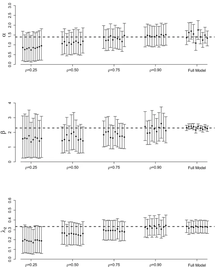
Figs2and3illustrate the posterior means and 95% credible intervals for each ILM parameter, for each of the 10 epidemics simulated. Averages of these results over the ten epidemic data sets are shown inS1 Table.

As expected, bias for all parameters decreases as the sampling proportion,ρ, increases under the SRS technique. Posterior variance also decreases asρincreases, leading to tighter credible intervals. It also appears to be more difficult to estimate the spatial parameterβusing an SRS scheme with precision approaching that seen under the full MCMC analysis than is the case withαandλ_z.

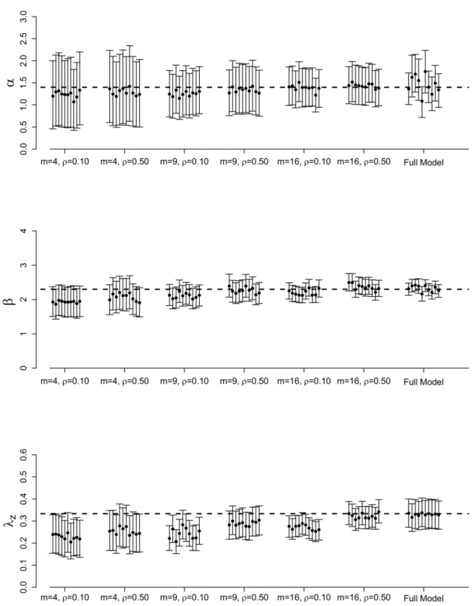
Introducing spatial stratification in our sampling scheme appears to lead to increased poste-rior accuracy (Fig 3). Under these results (shown forρ= 0.10 andρ= 0.50), as the number of strata,m, increases, posterior variance and bias decrease and, thus, credible intervals are tigh-ter. The posterior means also tend to be closer to the true parameter values. We also observe that spatial stratification is less sensitive to differentρvalues tested and more sensitive to differ-ent values form. For example, inFig 3, the posterior results forαunderm= 4 show almost no change forρ= 0.10 versusρ= 0.50. However, increasing the number of strata tom= 9 does increase posterior accuracy compared tom= 4. Under both values ofρ, we are able to obtain more posterior accuracy under the spatial stratification scheme than the simple random sam-pling scheme, demonstrating the advantage that including spatial stratification presents.

However, although spatial stratification appears more desirable in terms of posterior approximation, we must also consider the computation time required for the MCMC to run.

Table 1displays the average computation time (in hours) of each of our sampling methods. We observe that it takes approximately 92.64 hours to run 20,000 MCMC iterations of the true model without any data sampling. However, if we introduce SRS and setρ= 0.25, we notice a drastic reduction in computation time; the MCMC takes only 36.48 hours to run. The compu-tation time increases whenρincreases, as expected. The same is true if we consider spatial stratification in our sampling scheme. We see that smaller values ofmyield faster run times, but the posterior approximation improves with largerm. Obviously, in practice, a trade off between posterior accuracy and computation time would be required.

FMD Model Fitting Results

Fig 2. Posterior results for full MCMC and SRS methods.Posterior means and 95% credible intervals forα,β, andλzfor the full MCMC and SRS methods for 10 different epidemics simulated from the data augmented spatial ILM with varying sampling proportions. The dashed, horizontal lines represent the true parameter values:α= 1.4,β= 2.3, andl_z¼1

3, with a population of sizen= 625.

Fig 3. Full posterior results for full MCMC and spatial stratification methods.Posterior means and 95% credible intervals forα,β, andλzfor the full MCMC and spatial stratification methods for 10 different epidemics simulated from the data augmented spatial ILM with varying values formandρ. The dashed, horizontal lines represent the true parameter values:α= 1.4,β= 2.3, andl_z¼1

3, with a population of sizen= 625.

under the full model asρis increased, similar to the findings of the simulation study. In general, we also observe that posterior variance decreases asρincreases, resulting in tighter credible intervals closer to those under the full full model (which are generally the most narrow). Once again, these results mimic those seen in the simulation study.

Considering the spatially stratified schemes, we draw similar conclusions to those seen in the simulation study. Posterior accuracy tends to increase, and posterior variances decrease, as the number of strata,m, increases. In fact, form= 16 we obtain posterior estimates that are very close to those seen under the full model for parametersϕs,ϕc, andλz. Credible interval

widths forϕsandβchange negligibly with regards to choice ofm. Further, although posterior

variance decreases asmincreases, the credible intervals obtained under SRS withm= 4 (the lowest number of strata) contain those seen under the full MCMC analysis, suggesting good approximate inference.

Comparing the two sampling schemes, we see that spatial stratification tends to yield more accurate results. For example, if we compare SRS atρ= 0.50 with stratification even atm= 4 (also sampled withρ= 0.50), we find that all parameters under the spatial stratification scheme provide very similar, or more accurate, posterior means and tighter credible intervals. Asm increases, as we have also seen, these SRS-based results improve even further.

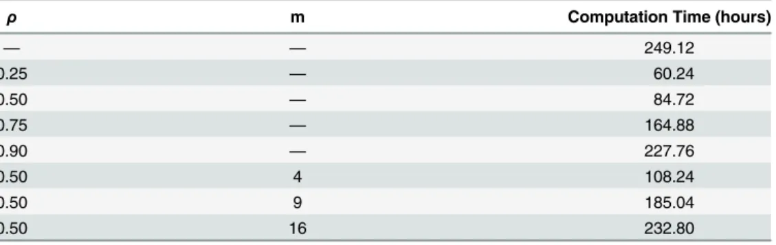
Once again, however, a key aspect in addition to modeling accuracy is reduction in compu-tation time.Table 2provides the run times (in hours) for each FMD data analysis. With the full model taking approximately 249.12 hours to run for 20,000 MCMC iterations, we notice signif-icant time savings atρ= 0.25 andρ= 0.50 using SRS and atm= 4 using spatial stratification. The time savings are much lower and of more questionable benefit for largerρandm. Further, and once again, time savings achieved using these sampling methods would be expected to be greater for larger data sets (seediscussion).

Discussion

In this paper, we introduced sampling algorithms to help speed up the likelihood calculation for ILMs in a Bayesian MCMC framework. Unlike other proposed methods (e.g., [8,12]), ours incorporates data augmented MCMC to allow for uncertainty about infection times into our analysis. We test the usefulness of our methods by comparing ILM parameter estimation under

Table 1. Average computation time for the simulation studies.

ρ m Computation Time (hours)

— — 92.64

0.25 — 36.48

0.50 — 47.76

0.75 — 59.28

0.90 — 75.12

0.10 4 46.88

0.50 4 56.16

0.10 9 66.24

0.50 9 71.52

0.10 16 82.32

0.50 16 88.56

Average computation run times (in hours) offitting the data augmented spatial ILM, SRS-ILM, and the SSS-ILM to 10 different simulated epidemics. These epidemics were simulated using ILM parametersα= 1.4,β= 2.3,l_z¼1

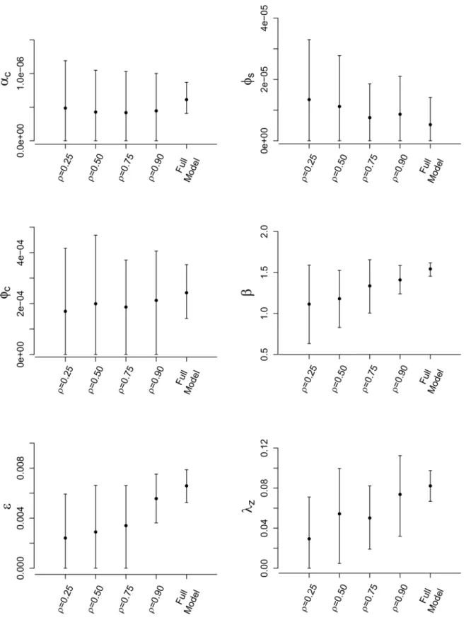
Fig 4. Posterior results for FMD-ILM using the SRS method.Posterior means and 95% credible intervals for all parameters of the data augmented FMD-ILM under the SRS method. The results are compared to the full model to assess accuracy.

the full Bayesian analysis via a simulation study and using data from the 2001 FMD epidemic in the U.K. Our results show that overall, we were able to obtain fairly accurate (though less precise) results using sampling-based likelihood approximations compared to the results obtained under the full likelihood analysis. In terms of computation run times, we found signif-icant savings could be made by using data sampling. Because the problem of repeated likeli-hood calculations under the full model is increased drastically with the inclusion of data augmentation, this is a result of key importance. However, we found using larger values ofρor mcan drastically reduce the time saving benefit over the full MCMC analysis.

In our studies, only two sampling techniques were considered. Possible future work could involve investigating other sampling procedures that might provide stronger inferential con-clusions. For example, our spatial stratification technique consisted of dividing the population into equally sized cells/strata and then sampling from each cell with equal sampling propor-tions. This would seem intuitively sensible when the population is spread across a grid, as was the case in our simulation study. This may be reasonable for some crop diseases or perhaps if points on the grid represent regions or cells (e.g., consider the modeling of fire spread by [23]), but such a population layout would be quite unrealistic in most situations. (It was, of course, adequate for the main aim of this paper, which was to illustrate the facilitation of faster likeli-hood calculations via data sampling).

In most populations, some natural clustering of individuals tends to take place (e.g., there tend to be high density clusters of farms in regions where infrastructural and/or environmental conditions are suitable for the type of farming in question). In such situations, spatial strata could, for example, be based upon some spatial clustering method applied to the population data. Alternatively, for a population in which some sort of contact network, or series of such networks, were being used as a prime risk factor in the model, clustering based on the network (s), using say partitioning around medoids (PAM) [24], could be considered as a way of defin-ing strata from which to sample.

Here, we assumed that the sampling proportion was invariant to time and/or stratum. How-ever, it might be useful to allow the sampling proportion to vary according to one or both. We might also possibly want to place more weight on sampling at times when the epidemic inten-sity is highest. Alternatively, in the case of spatially stratified sampling, we might want to avoid sampling from some strata with very low epidemic intensity. Such methods could possibly pro-vide faster computation concurrent with more accurate model parameterization.

There are also, of course, many other options for carrying out approximate inference when computational efficiency is a driving factor. For example, [25] use a Gaussian process emulator

Table 2. Computation times for the FMD-ILM.

ρ m Computation Time (hours)

— — 249.12

0.25 — 60.24

0.50 — 84.72

0.75 — 164.88

0.90 — 227.76

0.50 4 108.24

0.50 9 185.04

0.50 16 232.80

Computation run times (in hours) offitting the data augmented FMD-ILM to the FMD data using various sampling techniques. Models produced 20,000 realizations from the posterior.

method based on mapping key summary statistics from model simulations to the parameter space. In a similar vein, the aforementioned so-called approximate Bayesian computational methods used by, for example, [14] and [15], can be employed. These are also based on com-paring salient summary statistics from observed and simulated data. A systematic comparison of all of these different approaches would be of obvious interest.

Our study used aSIRmodeling framework. We could extend the analysis presented here to aSEIRframework to investigate disease exposure times. In our modeling, we accounted for incubation by treating it as a period when infected individuals have not been diagnosed yet but can pass on the disease to others. Introducing an exposed state would indicate an individual has contracted the disease but cannot pass it on to others until they reach the infectious state, regardless of confirmation of disease diagnosis. Additionally, we assumed knowledge of when individuals were removed from the population; however, this would not be the case for most diseases (e.g., human influenza). In a future study, we can also explore scenarios where removal times are unknown and instead estimated through data augmentation. The modeling frame-work used in this paper was also set in discrete time. The time saving sampling used here can also be applied in a (more natural, arguably) continuous time modeling framework.

We have demonstrated as a proof of concept that, for these relatively small datasets, our sampling-based likelihood approximations can result in a significant decrease in computation time. The time savings using these sampling algorithms would be even more beneficial in large-scale problems involving massive data sets compared to a full Bayesian analysis. A natural avenue of possible future work would be to apply these techniques to much larger data sets. Of course, these techniques would only really be worth using for large data sets in which a full Bayesian analysis was computationally prohibitive, in which case the priority would likely to be to get some sort of‘rough and ready’inference done as quickly as possible, rather than worry too much about the quality of posterior approximation. However, some degree of thought would have to be given to the choice ofρand the stratification methods used in order to achieve parametrization of a reasonable quality in a feasible time frame. Further work on the use of some sort of adaptive scheme, based initially on a quick pilot study over sampling pro-portions and stratification schemes, might also therefore be of interest.

Supporting Information

S1 Table. Summary statistics for the simulation studies.Summary statistics from the simula-tion studies comparing model parameter estimasimula-tion across our different sampling schemes. The results are averaged over 10 different epidemics simulated from the data augmented spatial ILM with parameter valuesa¼1_:4_;b¼2_:3_;l

z¼

1

3, andn= 625. Here, CIs are the mean

cred-ible interval limits. (PDF)

S2 Table. Summary statistics for modeling the FMD-ILM.Summary of results from fitting the data augmented FMD-ILM to the FMD data. We compare the results across our different sampling methods. Note that for spatial stratification, we sampleρ= 0.50 from each stratum. (PDF)

Author Contributions

References

1. Sun GQ. Pattern formation of an epidemic model with diffusion. Nonlinear Dynamics. 2012; 69 (3):1097–1104. doi:10.1007/s11071-012-0330-5

2. Sun GQ, Liu QX, Jin Z, Chakraborty A, Li BL. Influence of infection rate and migration on extinction of disease in spatial epidemics. Journal of Theoretical Biology. 2010; 264(1):95–103. doi:10.1016/j.jtbi. 2010.01.006PMID:20085769

3. O’Neill PD. Introduction and snapshot review: relating infectious disease transmission models to data. Statistics in Medicine. 2010; 29(20):2069–2077. doi:10.1002/sim.3968PMID:20809536

4. Shekhar S, Evans MR, Kang JM, Mohan P. Identifying patterns in spatial information: a survey of meth-ods. WIREs Data Mining and Knowledge Discovery. 2011; 1:193–214. doi:10.1002/widm.25

5. Chis Ster I, Ferguson NM. Transmission parameters of the 2001 foot and mouth epidemic in Great Brit-ain. PLoS ONE. 2007; 2(6):e502. doi:10.1371/journal.pone.0000502PMID:17551582

6. Chis Ster I, Singh BK, Ferguson NM. Epidemiological inference for partially observed epidemics: the example of the 2001 foot and mouth epidemic in Great Britain. Epidemics. 2009; 1(1):21–24. doi:10. 1016/j.epidem.2008.09.001PMID:21352749

7. Jewell CP, Kypraios T, Neal P, Roberts GO. Bayesian analysis for emerging infectious diseases. Bayesian Analysis. 2009; 4(2):191–222.

8. Deardon R, Brooks SP, Grenfell BT, Keeling MJ, Tildesley MJ, Savill NJ, et al. Inference for individual level models of infectious diseases in large populations. Statistica Sinica. 2010; 20(1):239–261. PMID: 26405426

9. Malik R, Deardon R, Kwong GPS, Cowling BJ. Individual-level modeling of the spread of influenza within households. Journal of Applied Statistics. 2014; 41(7):1578–1592. doi:10.1080/02664763.2014. 881787

10. Gamerman D, Lopes HF. Markov Chain Monte Carlo: Stochastic Simulation for Bayesian Inference. 2nd ed. Chapman & Hall/CRC Texts in Statistical Science. CRC Press; 2006.

11. Daley DJ, Gani J. Epidemic Models: An Introduction. Cambridge University Press; 2001.

12. Kwong GPS, Deardon R. Linearized forms of individual-level models for large-scale spatial infectious disease systems. Bulletin of Mathematical Biology. 2012; 74(8):1912–1937. doi: 10.1007/s11538-012-9739-8PMID:22718395

13. Brown PE, Chimard F, Remorov A, Rosenthal JS, Wang X. Statistical inference and computational effi-ciency for spatial infectious disease models with plantation data. Journal of the Royal Statistical Soci-ety: Series C (Applied Statistics). 2013.

14. McKinley T, Cook AR, Deardon R. Inference in epidemic models without likelihoods. The International Journal of Biostatistics. 2009; 5(1): Article 24. doi:10.2202/1557-4679.1171

15. Toni T, Welch D, Strelkowa N, Ipsen A, Strumpf MP. Approximate Bayesian computation scheme for parameter inference and model selection in dynamical systems. Journal of the Royal Society Interface. 2009; 6:187–202. doi:10.1098/rsif.2008.0172

16. McKinley TJ, Ross JV, Deardon R, Cook AR. Simulation-based Bayesian inference for epidemic mod-els. Computational Statistics & Data Analysis. 2014; 71:434–447. Available from:http://www. sciencedirect.com/science/article/pii/S016794731200446X. doi:10.1016/j.csda.2012.12.012

17. Manolopoulou I, Chan C, West M. Selection sampling from large data sets for targeted inference in mix-ture modeling. Bayesian Analysis. 2010; 5(3):429–450. doi:10.1214/10-BA517

18. Cauchemez S, Ferguson NM. Methods to infer transmission risk factors in complex outbreak data. Journal of the Royal Society Interface. 2012; 68(9):456–469. doi:10.1098/rsif.2011.0379

19. Metropolis N, Rosenbluth AW, Rosenbluth MN, Teller AH, Teller E. Equations of state calculations by fast computing machines. Journal of Chemical Physics. 1953; 21(6):1087–1092. doi:10.1063/1. 1699114

20. Hastings WK. Monte Carlo sampling methods using Markov chains and their applications. Biometrika. 1970; 57(1):97–109. doi:10.1093/biomet/57.1.97

21. Chib S, Greenberg E. Understanding the Metropolis-Hastings algorithm. The American Statistician. 1995; 49(4):327–335. doi:10.1080/00031305.1995.10476177

22. Anderson I. Foot and mouth disease 2001: Lessons to be learned inquiry. London: The Stationary Office; 2002.

24. Park HS, Jun CH. A simple and fast algorithm for K-medoids clustering. Expert Systems with Applica-tions. 2009; 36(2):3336–3341. doi:10.1016/j.eswa.2008.01.039