www.atmos-chem-phys.net/10/8499/2010/ doi:10.5194/acp-10-8499-2010
© Author(s) 2010. CC Attribution 3.0 License.
Chemistry
and Physics
A closer look at Arctic ozone loss and polar stratospheric clouds
N. R. P. Harris1, R. Lehmann2, M. Rex2, and P. von der Gathen2
1European Ozone Research Coordinating Unit, Department of Chemistry, University of Cambridge, Lensfield Rd,
Cambridge, CB2 1HE, UK
2Alfred Wegener Institute, Potsdam, Germany
Received: 24 December 2009 – Published in Atmos. Chem. Phys. Discuss.: 10 March 2010 Revised: 2 August 2010 – Accepted: 31 August 2010 – Published: 8 September 2010
Abstract. The empirical relationship found between column-integrated Arctic ozone loss and the potential vol-ume of polar stratospheric clouds inferred from meteorolog-ical analyses is recalculated in a self-consistent manner us-ing the ERA Interim reanalyses. The relationship is found to hold at different altitudes as well as in the column. The use of a PSC formation threshold based on temperature dependent cold aerosol formation makes little difference to the original, empirical relationship. Analysis of the photochemistry lead-ing to the ozone loss shows that activation is limited by the photolysis of nitric acid. This step produces nitrogen diox-ide which is converted to chlorine nitrate which in turn reacts with hydrogen chloride on any polar stratospheric clouds to form active chlorine. The rate-limiting step is the photolysis of nitric acid: this occurs at the same rate every year and so the interannual variation in the ozone loss is caused by the ex-tent and persistence of the polar stratospheric clouds. In early spring the ozone loss rate increases as the solar insolation in-creases the photolysis of the chlorine monoxide dimer in the near ultraviolet. However the length of the ozone loss period is determined by the photolysis of nitric acid which also oc-curs in the near ultraviolet. As a result of these compensating effects, the amount of the ozone loss is principally limited by the extent of original activation rather than its timing. In ad-dition a number of factors, including the vertical changes in pressure and total inorganic chlorine as well as denitrification and renitrification, offset each other. As a result the extent of original activation is the most important factor influencing ozone loss. These results indicate that relatively simple pa-rameterisations of Arctic ozone loss could be developed for use in coupled chemistry climate models.
Correspondence to: N. R. P. Harris
1 Introduction
Polar ozone loss has been the subject of intense scientific and public interest since the discovery of the Antarctic ozone hole (Farman et al., 1985) and its relatively quick attribution to observations of chlorine compounds (de Zafra et al., 1987; Solomon et al., 1987; Anderson et al., 1989). Stratospheric ozone loss takes place in the polar vortex which forms over each pole in their respective winters. Marked differences in stratospheric dynamics in the two hemispheres naturally lead to large interannual variations in vortex stability and in ozone in the dynamically active Arctic winter stratosphere and to small interannual variations in the dynamically less active Antarctic. These differences lead to higher natural average amounts of total ozone over the Arctic (∼450 Dobson Units – DU) than over the Antarctic (∼300 DU – Dobson, 1968; Newman and Rex, 2007). These differences in dynamics also lead to a much greater variability of polar ozone loss over the Arctic (where, for example, there were losses of<10% in 1998/1999 (Schulz et al., 2001) and>65% in 1999/2000 (Rex et al., 2002) at around 18 km) than over the Antarctic where nearly complete ozone loss has taken place in nearly all winters since the early 1990s at altitudes between about 15 and 20 km. Even in the anomalous year of 2002 when the Antarctic vortex was disturbed and broke up just after the middle of September, the minimum daily total ozone value south of 40◦S was∼140 DU, 30% below the late July values (Bodeker et al., 2005), and losses of 70–75% had occurred between the 400 and 500 K isentropic surfaces (Hoppel et al., 2003; Ricaud et al., 2005). In percentage terms this loss is comparable with the largest losses observed in the Arctic.
available, although 3-D chemical transport models (CTMs – e.g., Chipperfield et al., 2005) and data assimilation ap-proaches (Jackson and Orsolini, 2008) have been continually improving. However the additional complication of calculat-ing the stratospheric dynamics (coupled with the sensitivity of the ozone loss processes to the dynamics and transport) means that it is even harder to predict Arctic ozone losses for the coming decades using coupled chemistry climate mod-els (CCMs) (Austin et al., 2003; Eyring et al., 2007). The sensitivity of ozone loss to changes in climate is thus hard to assess.
The basic mechanisms leading to ozone loss are the same over the two poles and are generally well understood (e.g., Newman and Rex, 2007). As the polar vortex is estab-lished, the temperatures drop below a critical point, and po-lar stratospheric clouds (PSCs) can form. HCl and ClONO2
react on the surface of PSCs, with these unreactive chlo-rine species being converted under sunlit conditions to ac-tive forms (ClOx= ClO + 2·Cl2O2) which can rapidly destroy
ozone. In the absence of further exposure to PSCs, the ClO (chlorine monoxide) formed continues to destroy ozone while it is gradually converted back to unreactive forms. The observed evolution of the main chemical species in the Arc-tic can be seen in Fig. 1 for the 2004/2005 winter. The concentrations of HCl and ClONO2 decrease in the
pres-ence of PSCs, while the inferred concentration of ClOx
in-creases. (Note that ClOxin Fig. 1 is calculated as Clyminus
ClONO2and HCl so it includes minor species such as HOCl
and Cl2.) Continued PSC occurrence leads to continued
for-mation of ClOxuntil the HCl is low. Reversion of ClOx to
ClONO2and HCl occurs as the vortex warms and the PSCs
evaporate. Occasionally in Arctic winters, particularly large ozone losses can occur when air masses become depleted in HNO3as PSCs sediment to lower altitudes during prolonged
cold periods, a process that delays the deactivation of the ac-tive chlorine species. The persistence of PSCs depends very strongly on the dynamical situation in that winter and so is the main reason that ozone loss can vary so much from year to year in the Arctic.
Given the mechanistic complexity and large variability, it came as a surprise to find that a compact, linear relation ex-ists between ozone loss and the calculated volume of PSCs (VPSC) when each is integrated over the period of vortex ex-istence (Rex et al., 2004, 2006). The relation holds over a wide range of ozone losses and PSC volumes implying that the effects of many influences on ozone loss (e.g., denitrifica-tion, solar exposure, initial chemical fields, descent rates, in-mixing, vortex inhomogeneities, and vertical extent) must be offsetting to some extent. The existence of this relation (cal-culated from temperature fields and vortex average descent rates derived from meteorological analyses and ozonesonde measurements) has been confirmed using HALOE satellite measurements and an independent approach to calculating the ozone loss (Tilmes et al., 2004). Both Rex et al. (2004) and Tilmes et al. (2004) found larger than expected chemical
Fig. 1. Evolution of chlorine species inside the Arctic vortex at
460 K in the 2004/2005 winter. The top panel shows the area of PSCs as a percentage of the vortex area (light blue) and the vortex average sunlit time per day in percent (pink). PSCs are assumed to be NAT and the area is calculated from ECMWF analyses. A value of 36 s−1normalized potential vorticity is used to define the edge of the vortex (see Rex et al., 1999). This value is close to the maximum horizontal gradient in normalized PV between early January and late March. The middle panel (based on Santee et al., 2008) is the vortex average HCl from Aura MLS, the vortex average ClONO2
from ACE FTS, and an estimate of the vortex average ClOxfound
by subtracting the sum of the HCl and ClONO2from 2.8 ppb, a
rep-resentative value of Clyfor 460 K in that winter. ClONO2and ClOx
have been smoothed with a 10 day running mean in order to com-pensate for the sampling biases from ACE FTS, which has the typi-cal sampling issues of any solar occultation instrument. The bottom panel shows the ozone loss rates found from the Match campaign for that year (Rex et al., 2006).
ozone losses in the 1991/1992 and 1992/1993 winters which they attributed to the increase in stratospheric aerosol follow-ing the eruption of Mt Pinatubo.
et al., 2005, updated at http://www.pa.op.dlr.de/CCMVal/ CCMVal EvaluationTable.html; SPARC CCMVal, 2010), despite its empirical robustness and the implication that there is a sensitivity of 15 DU column ozone loss for each 1◦C cooling (Rex et al., 2006). The relation has however been used to evaluate (a) the improvements made to the SLIM-CAT 3-D Chemical Transport Model (CTM) which previ-ously showed a compact, linear relation of the wrong slope (Rex et al., 2004), and now can reproduce the slope as well (Chipperfield et al., 2005; Fig. 4.13 in Newman and Rex, 2007), and (b) the ozone loss calculated in the Whole Atmo-sphere Community Climate Model (WACCM) (Tilmes et al., 2007).
The aim of this paper is to explain the compactness and linearity of this relationship and to unravel the important fac-tors already present in the models as well as in the atmo-sphere. We are not trying to reproduce the observed relation quantitatively – that has already been done in more sophisti-cated models. We therefore choose to use a relatively simple tool (a photochemical box model with idealized trajectories) to identify the main processes rather than a more complex model which is harder to diagnose. Our earlier work (Harris et al., 2009) found that the rate-determining step for chlorine activation is the photolysis of HNO3, while the subsequent
ozone loss depended on the competition between the pho-tolysis of Cl2O2(leading to ozone loss) and HNO3(leading
to deactivation). Since both processes go faster as the so-lar zenith angle decreases, the integrated ozone loss depends primarily on the extent of the initial chlorine activation and not on the speed of the ozone loss. Here we investigate the empiricalVPSC /ozone loss relationship in more detail using ERA Interim reanalyses and looking at its altitude depen-dence, and we extend the photochemical analysis to investi-gate the effect of multiple activations, denitrification and the vertical distribution of available chlorine (Cly).
In the next section the methodology and data sources are described. In Sect. 3, the altitude variation of the relation is investigated and the sensitivity to the assumptions about PSC composition are discussed. The critical photochemical steps involved in the activation and deactivation steps are then de-scribed and illustrated in Sect. 4 by photochemical calcula-tions on a single surface. Three dimensional aspects are dis-cussed in Sect. 5. Finally the relevance and context of these results is discussed and summarised in Sect. 6.
2 Methodology
This study uses the values for ozone loss andVPSC calcu-lated in Rex et al. (2006) updated with values for 2005/2006, 2006/2007 and 2007/2008 using the same methodology. Vor-tex averaged profiles of ozone loss have been determined as the differences between ozone mixing ratio profiles at the end of March and early January, with an adjustment for the vor-tex average descent being made using diabatic heating rates
from the SLIMCAT CTM. These have been converted into concentration versus altitude profiles, using the vortex aver-aged temperature and pressure profiles from late March. The total column loss was calculated as the vertical integral of the loss profiles between 14 and 24 km in March. The lower limit of this range (∼380 K) is close to the bottom of the well-isolated part of the polar vortex. For most winters ozone loss at this level is small. Also, the effect of any chemical loss in the vertical region below 14 km on the total ozone column in the Arctic would be limited because of rapid exchange with mid latitude air. Formation of PSCs above the vertical range considered here is unlikely (Pitts et al., 2009), and conse-quently significant chemical loss of ozone is not expected to be seen in air masses at or above 24 km at the end of winter. (Note that in our analysis we are using end of winter alti-tudes as a reference and that airmasses have descended from higher altitudes.) The estimated uncertainty in the integrated ozone loss is∼10–15 DU (Rex et al., 2002), mainly due to uncertainties in the calculated cooling rates and the potential impact of mixing across the vortex edge.
PSCs are assumed to be nitric acid trihydrate (NAT), and VPSCis calculated from the laboratory observations of Han-son and Mauersberger (1988), a water vapour mixing ratio of H2O = 5 ppm, and an observed profile of HNO3(see Rex
et al., 2002 for more details and discussion of the methodol-ogy). In this paper temperatures from ECMWF ERA-Interim re-analyses are used in order to have a consistent vertical res-olution and data quality across the whole period. The validity of this approach, particularly the assumptions made about the composition of PSCs, is discussed further in Sect. 3.
In order to investigate the underlying processes, the Al-fred Wegener Institute (AWI) photochemical box model was used. This model contains 48 chemical species and 174 re-actions. The formation of solid and liquid PSC particles is simulated according to Murray (1967), Hanson and Mauers-berger (1988) and Carslaw et al. (1995). For the photolysis of Cl2O2, the absorption cross sections from Burkholder et
al. (1990) are used, which are close to the values found in the most recent laboratory studies (Chen et al., 2009; Pa-panastasiou et al., 2009; von Hobe et al., 2009). All remain-ing information on rate constants is taken from the NASA-JPL 2006 Evaluation (Sander et al., 2006). The overhead ozone needed for the calculation of photolysis frequencies is the average of all ozonesonde measurements made be-tween January and March from 1992–2007 at Ny-Alesund (79◦N). The numerical integration is performed using the kinetic preprocessor KPP (Damian et al. 2000). Unless oth-erwise stated, the model is initialised with HCl = 2.25 ppb, ClONO2= 0.75 ppb (consistent with Fig. 1), ClOx= 0 ppb,
HNO3= 10 ppb, NOx= 0, H2O = 3.5 ppm, O3= 3 ppm and
Bry= 20 ppt.
Fig. 2. Integrated ozone loss as a function ofV
PSCfor 1992/1993 to
2008/2009. Ozone losses are derived from the Arctic ozonesonde network using the vortex average approach. No meaningful ozone losses could be calculated in the winters 2000/2001, 2001/2002, 2003/2004, 2005/2006 and 2008/2009 due to major warmings over-lapping with the ozone loss period and/or lack of ozonesonde data. The error bars associated with the ozone loss values reflect a con-servative estimate of 20 DU (e.g. Newman and Rex, 2007).V
PSCis
derived from ECMWF ERA-Interim re-analyses using the temper-ature of formation of nitric acid trihydrate. The error bars onV
PSC
show the sensitivity to a temperature perturbation of±1 K in the ECMWF data. (Updated from Rex et al., 2006).
edge of an Arctic vortex which is centred at 80◦N towards Europe with a radius corresponding to 20◦(as often encoun-tered in reality). The airmass thus moves around the vortex with latitudes ranging from 60◦N above Europe over the pole to 80◦N above the Aleutians, taking 6 days to do so (a typ-ical time for one circum-navigation). The main set of runs is performed at 50 hPa (∼475 K). Runs investigating the ver-tical dimension were performed at 550 K (∼30 hPa), 500 K (∼40 hPa) and 450 K (∼55 hPa). The analysis presented here is split into three main parts: the activation period (Sect. 4.1); the ozone loss period (Sect. 4.2); and aspects of the vertical dimension process (Sect. 5).
3 Altitude variation of relation and PSC composition
The original plots of integrated column ozone loss against integrated PSC volume (Rex et al., 2004, 2006) were calcu-lated using ECMWF operational analyses. The PSC volumes shown in Fig. 2 are calculated using ERA-Interim re-analyses (Simmons et al., 2006). These give greater consistency be-tween years. The general features of the plot are unchanged. The most notable change is that the largest value forVPSC is now calculated to be in 1995/1996 rather than 2004/2005. The slope of a linear fit between ozone column loss andVPSC is slightly reduced. All these changes are within the estimate uncertainties.
Figure 3 shows the ozone loss on individual isentropic sur-faces (400, 450, 500 and 550 K) plotted against the area of PSCs (APSC), both integrated over the course of the win-ter. (As for the column ozone loss and VPSC, the
isen-Fig. 3. Integrated ozone loss for individual subsiding surfaces
de-rived with the approach described in Rex et al. (2006) as a function ofAPSC for 1992/1993 to 2008/2009. The potential temperature
shown in each panel is the spring equivalent potential temperature which is the value of the subsiding layers at the end of winter. Other details are given in the caption for Fig. 2. We estimate that the ab-solute uncertainties associated with the ozone loss at 400, 450 and 500 K are±0.75×10¹²molec cm−3 and ±0.5×10¹²molec cm−3 at 550K where there is less sensitivity to errors in the diabatic cool-ing. The relative uncertainty associated with APSCis estimated to be±20%.
550 K (0.26±0.057, 0.15±0.041 molec cm−3/million km2,
respectively), showing the importance of the lower levels to the integrated column loss. The 550 K plot has the largest relative scatter. This is partly due to the smaller ozone losses found there and partly due to the poorer data quality (a sig-nificant fraction of ozonesondes do not reach that high espe-cially early in winter as the descending layer starts at 600 or 700 K).
VPSCand APSCin Figs. 2 and 3 are meant as proxies for the geographical extent of conditions favourable for chlorine activation. The values in these plots are derived from mete-orological analyses based on a threshold temperature for the existence of such conditions. The particular numerical val-ues in the plots show the results for using the NAT equilib-rium temperature (TNAT) as threshold. The formation of STS is a gradual process without such a clear threshold. But the efficiency of chlorine activation on STS is a steep function of temperature and the NAT equilibrium temperature is very close to the small range of temperatures at which the chlorine activation on STS becomes efficient on timescales of days or hours. So usingTNATas the proxy for chemical processing due to heterogeneous reactions is meaningful even though the real process of activation is more complicated and in-volves different types of droplets or particles in the strato-sphere. The composition of large-scale fields of PSCs has been recently investigated using the MIPAS infrared sounder and the CALIPSO/CALIOP lidar measurements (H¨opfner et al., 2009; Pitts et al., 2007, 2009). They find that the PSC fields can be described by four main types (ice, NAT-STS mixtures, STS-ICE mixtures, and just STS). The overall evo-lution of the observed PSCs is similar to that deduced from meteorological analyses. In the Antarctic (their main focus) they find that the PSC occurrences calculated from meteo-rological analyses are 30–40% less than their observations. However it is hard to make quantitative comparisons. Pitts et al (2009) use observed HNO3and H2O fields to calculate
possible PSC existence while we assume a temporally un-varying concentration profile. In the Antarctic they observe significant amounts of optically thin NAT which are at the threshold limit of their instruments. A closer examination of these issues in the Arctic is needed to see if these findings are also valid there.
The effect of usingTNATas the temperature threshold for calculating our PSC proxy was investigated by Tilmes et al. (2008). They introduced a PSC proxy based on a temper-ature threshold for the activation of chlorine on STS and cold background aerosol and investigated the effect of using this PSC formulation on the ozone loss/VPSCrelation. Significant differences were only found in winters with high sulphate aerosol loading, i.e. 1991/1992 and 1992/1993 following the Mt Pinatubo eruption. For comparison, we have used the temperature dependent cold aerosol formation to calculate APSC(as in Fig. 3, but not shown). No meaningful difference
is found except ateθ= 400 K, where there is a slightly more compact relation with a correspondingly higher R2 value.
This is presumably related to the higher amount of back-ground aerosol at these altitudes. This is consistent with the CALIOP analysis in the Antarctic which shows the biggest discrepancy in a 1–2 km band at altitudes below 15 km at the beginning of winter (Fig. 14c in Pitts et al., 2009). A similar feature can be seen in the comparison of calculated PSC oc-currence usingTNATwith ground-based lidar observations in 1999/2000 Arctic winter (Fig. 2 in Rex et al., 2002). Over-all we conclude thatVPSC andAPSC calculated using NAT existence are good proxies for the existence of PSCs, the ac-tivation of chlorine and for threshold conditions for ozone loss.
4 Idealised case: a single layer
We now examine the relationship of the ozone loss to the photochemical steps involved in the activation and deactiva-tion of ClOxat 50 hPa using the AWI box model. In section
4.1 we discuss the effects of the frequency of occurrence and temperature of the PSCs; while in Sect. 4.2 we investigate the competition between the ozone loss and ClOx
deactiva-tion chemistry. 4.1 Activation
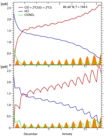
Figure 4a shows the mixing ratios of the chlorine reservoirs, ClONO2and HCl, and the activated forms ClOxfrom 1
De-cember to 14 February assuming that PSCs are continuously present. The assumed temperature is 194 K which is rep-resentative of the vortex as a whole. Two phases can be seen: (i) a rapid initial rise in ClOx associated with equal
decreases in both HCl and ClONO2; and (ii) a slower
contin-ued increase in ClOxaccompanied by a continued decrease
in HCl. By the end of the period, nearly all the available chlorine is in the form of ClOx. ClOx rises initially as a
result of the fast heterogeneous reaction between ClONO2
and HCl, with the extent of the initial activation being deter-mined by the amount of ClONO2initially present (M¨uller et
al., 1994; Santee et al., 2008). The heterogeneous reaction of ClONO2+ HCl proceeds quicker at lower temperatures, and
the main effect of lower temperatures is thus to accelerate the initial activation (Fig. 4b).
If the initial mixing ratio of HCl is greater than that of ClONO2, further activation depends on the formation of
more ClONO2 (e.g., M¨uller et al., 1994) which depends in
turn on the photolysis of HNO3 producing NO2 which
re-acts with ClO to form ClONO2. In the presence of PSCs, the
ClONO2reacts rapidly with HCl to produce more ClOx. In
the Arctic winter the slow step in the overall activation mech-anism is the photolysis of HNO3, with a timescale of days to
weeks.
ClONO2+HCl het
→Cl2+HNO3 (R1)
Fig. 4. (a) The evolution of (ClOx+ 2Cl2), HCl and ClONO2for an
idealised trajectory at a temperature of 194 K and 50 hPa with con-tinued activation from 1 December to 14 February. The latitude of the trajectory oscillates around 80◦N with a 20◦amplitude. The or-ange shading indicates the sunlight exposure experienced by the air parcel. (b) The same for an idealised trajectory at 50 hPa with a one day period of activation at 192 K every six days from 1 December to 14 February.
NO2+ClO+M→ClONO2+M. (R3)
The slow, continued rise in ClOx in Fig. 4 thus depends
principally on the photolysis frequency,J(HNO3), and this factor is responsible for the acceleration in the activation after mid-winter. The initial activation is also faster if the ClONO2:HCl ratio is closer to unity. If significant chlorine
activation occurs, Reaction (R3) is sufficiently fast that most of the NO2 produced by the photolysis of ClONO2 reacts
back to ClONO2with a time constant of a few minutes, and
so the ClONO2photolysis can be disregarded in these
condi-tions.
In the real Arctic vortex, the initial activation is patchy depending on the altitudes and regions where the PSCs first form as well as on their extent. Vortex average ClOxinitially
rises slower in reality than in the idealised case, as indicated in Fig. 1. To illustrate this, Fig. 4b shows the same model calculation as in Fig. 4a, except that the PSCs occur episodi-cally (1 day in 6) and at temperatures of 192 K. The
stabilisa-Fig. 5. The photolysis frequencies of HNO3and Cl2O2at 50 hPa in the Arctic vortex as a function of solar zenith angle.
tion of HCl between PSC exposures is a result of the lack of PSCs. Each of the small rises in ClOxresults from exposure
to PSCs, and the decreases occur during exposure to sunlight (orange). The overall shape is still determined byJ(HNO3). Further, the initial rapid activation could be responsible for the non-zero intercepts in Figs. 2 and 3, as any small-scale or sub-grid process leading to PSC formation (e.g. mountain waves) could rapidly activate a small but significant amount of air while barely contributing toVPSC.
Overall, our analysis of the chlorine activation shows that activation in Reaction (R1) is fast and that the rate limiting factor for any continued activation is the photolysis of HNO3
to form NO2 in Reaction (R2) and then ClONO2in
Reac-tion (R3). To first order the photolysis of HNO3 does not
vary much from year to year, and so interannual variations in activation depend on the presence of PSCs for activation to occur through Reaction (R1).
4.2 Deactivation and ozone loss
There have not been many studies explicitly looking at how the amount of ozone loss depends on the timing and extent of the initial activation. The main ozone loss period starts early in the year as the insolation increases. The instanta-neous ozone loss rates have been observed to peak in late January with a gradual reduction thereafter (von der Gathen et al., 1995). The daily ozone loss rate maximises a little later as it is also determined by the length of the day which is increasing in this period. As discussed in Harris et al. (2009), both the ozone loss and the chlorine deactivation are driven by sunlight and so the ozone loss and chlorine deactivation processes accelerate as the insolation increases. The rate lim-iting step for ozone loss in the Arctic (for a given amount of total inorganic chlorine (ClOx)) is:
Cl2O2+hν→ClOO+Cl (R4)
while in the absence of PSCs, Reactions (R2) and (R3) be-come the main deactivation mechanism.
Both HNO3 and Cl2O2 are photolysed in the UV, and
Fig. 6. Ozone mixing ratios calculated for an air parcel with an
ini-tial chlorine activation of 3 ppb ClOxon 11 January (red), 1
Febru-ary (blue) and 22 FebruFebru-ary (green); and (b) the ozone loss rates for the same cases.
(R4) in the Arctic polar lower stratosphere depend mainly on wavelengths longer than 300 nm as shorter wavelengths are absorbed by stratospheric ozone.
Figure 5 shows these photolysis rates as a function of so-lar zenith angle. They both increase markedly as the soso-lar zenith angle decreases as winter turns into spring. To first or-der both the chlorine deactivation rate, which determines the duration of the ozone loss, and the instantaneous ozone loss rate are proportional to the insolation, with both processes having a timescale of several days at 70–75◦N in January and February. As a result the integrated ozone loss is, to first order, independent of the insolation and the timing of the ac-tivation, but is dependent on the original level of activation.
The effect of the timing of activation on the ozone loss rates and on the ozone itself can be seen clearly in Fig. 6. All cases have an initial activation of 3 ppb of ClOxwith the
same hypothetical trajectory used before (50 hPa centred at 80◦N with 20◦deviation with a 6 day cycle). The only dif-ference is in the start dates which are set three weeks apart: 11 January (red), 1 February (blue) and 22 February (green). The later the activation, the larger the daily ozone loss, the shorter the period of ozone loss. Despite the large differences in the start dates and the evolutions of the ozone loss rates,
the cumulative ozone losses are within±10% (1.16 ppm for 11 January 1.10 for 1 February and 0.99 ppm for 22 Febru-ary).
While this analysis highlights the importance of the two photolysis Reactions (R2) and (R4) in determining ozone loss in the Arctic, other processes do play a limited role. For example, in Fig. 6 a smaller ozone loss is calculated when the 22 February start date is used. This is consistent with the greater sensitivity of the Cl2O2 photolysis rate to
decreas-ing SZA at high SZA (∼90◦) and the greater sensitivity of the HNO3photolysis rate at lower SZA (∼70–80◦) shown in
Fig. 5. Also, the conversion of HNO3to NOxvia the
alter-native channel
OH+HNO3→NO3+H2O (R5)
depends onJ(HNO3) since HNO3photolysis is the main for-mation pathway for OH in polar spring.
In addition, reactions which play an important role in Antarctic ozone loss are less significant in most Arctic win-ters. The highly temperatudependent, heterogeneous re-activation of ClONO2through
ClONO2+H2O→HOCl+HNO3 (R6)
is unimportant in most Arctic winters.
The sensitivity with respect to the calculated ozone loss with respect to the assumptions on the idealised trajecto-ries was investigated by repeating the model runs shown in Fig. 6 at two fixed latitudes, 65◦N and 75◦N. The differ-ence in the cumulative ozone losses for the three start dates was∼ ±10%, similar to the result found for the base case trajectory with varying latitudes. However, the ozone loss does depend on latitude: the greatest loss (1.3 ppm) was seen for the case where the trajectory started on 11 January at 75◦N, while the smallest (0.8 ppm) occurred when the tra-jectory started on 22 January at 65◦N. These variations also illustrate one of the reasons we chose base case trajectories which cover a realistic range of latitudes.
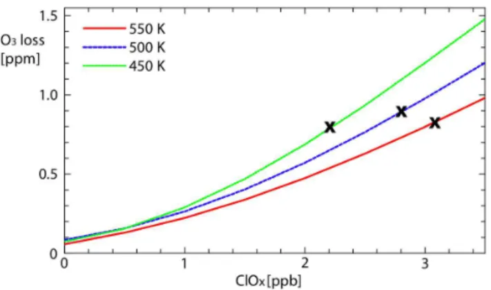
A further important point about the degree of activation is that the ozone loss is close to linear with ClOx. The blue line
in Fig. 7 shows the dependence of the accumulated ozone loss at 500 K (close to 50 hPa, the level of the calculations shown in Fig. 6) on the initial amount of ClOx. The
accumu-lated ozone losses for 1, 2 and 3 ppb ClOxat 500 K are 0.27,
0.59 and 1.00, respectively, so that there is a small, positive non-linearity in this relationship.
5 Extending to the 3-D view
Fig. 7. Integrated ozone loss as a function of initial activation on the
450 K (green), 500 K (blue) and 550 K (red) potential temperature surfaces. The crosses represent the amount of available inorganic chlorine in March 1992 inferred by Schmidt et al. (1994).
Cly with altitude; (3) the vertical redistribution of NOy in
de/renitrification; (4) the interannual variation of transport. 5.1 Dependence of reaction rate coefficients on pressure
(altitude)
For fixed ClOx, the potential for ozone loss depends slightly
on pressure, with larger ozone losses calculated at lower po-tential temperatures as shown in Fig. 7. For an initial ClOxof
3 ppb, the accumulated ozone losses at 450, 500 and 550 K are 1.2, 1.0 and 0.8 ppm. The reasons for the pressure depen-dence are as follows.
(a) At higher altitudes the ClO and BrO concentrations are smaller for the same mixing ratios, as is the overall pressure, thus reducing the rates of the reactions
ClO+ClO+M→Cl2O2+M (R7)
ClO+BrO→Br+Cl+O2. (R8)
(b) At higher altitudes the chlorine deactivation rate is higher, because NO2production through both HNO3photolysis and
(R5) is faster. An increase of the HNO3 mixing ratio with
altitude, not considered in the present model runs, would am-plify this effect.
Two possibly counteracting effects at higher altitudes are the faster rate of the reaction
ClO+O→Cl+O2 (R9)
because the O concentration increases with altitude; and the faster photolysis of Cl2O2(Reaction R4). However these are
small compared to points (a) and (b). 5.2 Available chlorine
The amount of available chlorine increases rapidly with al-titude in the Arctic vortex (Schmidt et al., 1994). As a re-sult, more chlorine is activated for a given PSC exposure at
higher altitudes. The black crosses in Fig. 7 indicate the val-ues of Clymeasured toward the end of the 1991/1992 winter
(Schmidt et al., 1994). Taking these as representative upper limits for the amount of ClOxinitially available shows that as
altitude increases the additional Clyoffsets the decreasing
ef-ficiency of the ozone loss processes. The combined effect is to limit the importance of any interannual variations of PSC altitudes on the integrated ozone loss.
5.3 Vertical Redistribution of NOy
The vertical redistribution of NOythrough denitrification at
higher altitudes and renitrification at lower altitudes has been widely cited as having a major impact on the accumulated ozone loss as the removal of NOy limits the deactivation of
ClOxthrough (R3). Significant denitrification in the Arctic
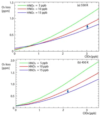
only occurs in a few winters (1994/1995 (Sugita et al., 1998); 1995/1996 (Rex et al., 1997); 1999/2000 (e.g., Popp et al., 2001) and 2004/2005 (Kleinb¨ohl et al., 2005)), which are the winters with the larger ozone losses in the top right of Fig. 2. Denitrification in the majority of winters is negligible, even non-existent. When large-scale denitrification does occur, the enhanced ozone loss in the denitrified layer tends to be offset by reduced ozone loss in a lower, renitrified layer (e.g. Rex et al., 1997). The magnitude of this effect is investigated here by assuming a denitrification at 550 K of 5 ppb (Fig. 8a) and a concurrent renitrification of 5 ppb at 450 K (Fig. 8b), similar to those reported by Popp et al. (2001). For a given ClOx, there is a greater sensitivity of ozone loss to changes
in NOyat 450 K than at higher altitudes (though note that the
cases shown are for similar changes in mixing ratio, not con-centration). However at this level, the Clyand ClOxare lower
and so the overall effect of this hypothetical de/renitrification on the vertically integrated ozone loss is limited. Interest-ingly (but not conclusively) if one looks at particular years in Fig. 3, one can see indications of both denitrification and renitrification. For example in 1999/2000, a year of extensive ozone loss and well observed denitrification, Fig 3b shows higher than “expected” ozone loss ateθ= 450 K and less than “expected” at 400 K, consistent with the altitudes of the ob-served denitrification/renitrification (Popp et al., 2001). 5.4 Interannual variations in transport
A further process which could affect the chemical recovery is any in-mixing of air with a different chemical composition from outside the vortex. Previous work indicates that this is not a significant influence on ozone loss in the Arctic vortex (Newman and Pyle, 2003) despite the identification of indi-vidual events (e.g., Pyle et al., 1994).
6 Discussion and summary
Fig. 8. The integrated ozone loss as a function of initial activa-tion on the (a) 550 K and (b) 450 K potential temperature surfaces. The green lines show the effect of HNO3= 5 ppb, the red lines for
HNO3= 10 ppb and the blue lines for HNO3= 15 ppb. The arrows
indicate the effect of a dentrification of 5 ppb at 550 K in (a) and a renitrification of 5 ppb at 450 K in (b).
potential PSC volume in the Arctic vortex (Rex et al., 2004, 2006; Tilmes et al., 2004) using the ERA-Interim reanalyses to calculateVPSC. Not only do the previous results still hold with additional winters and the self-consistent meteorolog-ical data set, but they are also shown to hold on individual potential temperature surfaces albeit with greater scatter. At eθ= 400 K, the relationship is found to be slightly more sig-nificant when cold aerosol activation is assumed in the place of NAT. This is consistent with the larger amounts of back-ground aerosol at 400 K than at higher altitudes. At higher potential temperatures, the correlation with PSC areas de-duced from NAT existence is better. This finding implies a smaller sensitivity of ozone loss to stratospheric aerosol load-ing than that found by Tilmes et al. (2008) in their assess-ment of the deliberate maintenance of an enhanced strato-spheric aerosol layer as a geo-engineering response to cli-mate change.
The compactness and linearity of the empirical results are interpreted using a photochemical box model with stan-dard photochemistry and idealised trajectories. The aim is to identify the important mechanisms, not to reproduce the losses from winter to winter. (More complete reconstruc-tions have been successfully reported elsewhere using a 3-D CTM and analysed meteorological fields (Chipperfield et al., 2005; Tilmes, 2007).) We show that the principal timescale
for the extensive activation of chlorine is not the fast reac-tion of ClONO2and HCl on NAT particles but the re-supply
of ClONO2with photolysis of HNO3 as the rate
determin-ing step. As a result, extensive activation in the Arctic vortex takes place with a timescale of days to weeks, and the overall activation depends on the continued (though not necessarily the continuous) presence of PSCs. The use ofVPSCis thus a sensible proxy for the activation process.
The extent of ozone loss in any particular winter is found to depend most strongly on the degree of activation and not so much on its timing or vertical distribution. This some-what surprising finding occurs as a result of a number of off-setting factors. For any given air mass, there is the almost cancelling competition between ozone loss and chlorine de-activation, both of which rely on the photolysis in the near UV and so accelerate as the Sun becomes higher in the sky in early spring. In the vertical, the effect of the decreasing num-ber density with altitude is offset by the increasing Cly
mix-ing ratios, and in the few winters where denitrification occurs the increased ozone loss at the denitrified altitudes is offset by the decreased ozone loss at the lower altitudes where re-nitrification takes place. The baroclinicity of the vortex af-fects the degree of denitrification (Mann et al., 2003): this would affect our conclusions about denitrification if the cold region were sufficiently deep that the renitrification occurred below the region of ozone loss. However this is very rare in the Arctic and has probably not occurred even in the years of extensive denitrification.
These findings raise a number of interesting possibilities for the development of simple parameterisations of strato-spheric Arctic (or even polar) ozone loss in coupled chem-istry climate models (CCMs), a step beyond the use of sim-ple models to investigate future sensitivities (Knudsen et al., 2004; Tilmes et al., 2008). For example, the relationship shown in Fig. 2, which is derived in a period of high and nearly constant Cly, could be scaled by the levels of Cly
calculated in the CCMs. As Cly decreases so will ozone
loss – but the effect of any changes in the occurrence of PSCs resulting from climate change would be allowed for. A slightly more sophisticated and intellectually more satis-fying approach based on processes would be to develop a simplified photochemical model based around the main fea-tures described above, namely photolysis of nitric acid and Cl2O2, an activation involving ClONO2 on PSCs, and the
initial levels of Cly. The success of either of these schemes
Acknowledgements. This work was supported by the EU Integrated
Project SCOUT-O3 (505390-GOCE-CT-2004) and by the BMBF DYCHO project (FKZ07ATC08). NRPH thanks NERC for an Advanced Research Fellowship. We thank the many ozonesonde personnel who have launched the ozonesondes used in this analysis. Michelle Santee and Peter Bernath provided useful and helpful advice. Meteorological data were provided by ECMWF and FU-Berlin. The ACE mission is supported primarily by the Canadian Space Agency. EOS Aura MLS is supported by NASA.
Edited by: M. Dameris
References
Anderson, J. G., Brune, W. H., and Proffitt, M. H.: Ozone destruc-tion by chlorine radicals within the Antarctic vortex: the spatial and temporal evolution of C1O-O3 anticorrelation based on in situ ER-2 data, J. Geophys. Res., 94(D9), 11465–11479, 1989. Austin, J., Shindell, D., Beagley, S. R., Br¨uhl, C., Dameris, M.,
Manzini, E., Nagashima, T., Newman, P., Pawson, S., Pitari, G., Rozanov, E., Schnadt, C., and Shepherd, T. G.: Uncertainties and assessments of chemistry-climate models of the stratosphere, Atmos. Chem. Phys., 3, 1–27, doi:10.5194/acp-3-1-2003, 2003. Bodeker, G. E., Shiona, H., and Eskes, H.: Indicators of
Antarctic ozone depletion, Atmos. Chem. Phys., 5, 2603–2615, doi:10.5194/acp-5-2603-2005, 2005.
Burkholder, J. B., Orlando, J. J., and Howard, C. J.: Ultraviolet absorption cross sections of Cl2O2between 210 and 410 nm, J.
Phys. Chem., 94, 687–695, 1990.
Carslaw, K. S., Luo, B., and Peter, T.: An analytic expression for the composition of aqueous HNO3-H2SO4stratospheric aerosols
including gas phase removal of HNO3, Geophys. Res. Lett., 22,
1877–1880, 1995.
Chen, H.-Y., Lien, C.-Y., Lin, W.-Y., Lee, Y. T., and Lin, J. J.: UV absorption cross sections of ClOOCl are con-sistent with ozone degradation models, Science, 324, 781, doi:10.1126/science.1171305, 2009.
Chipperfield, M. P., Feng, W., and Rex, M.: Arctic ozone loss and climate sensitivity: Updated three-dimensional model study, Geophys. Res. Lett., 32, L11813, doi:10.1029/2005GL022674, 2005.
Damian, V., Sandu, A., Damian, M., Potra, F., and Carmichael, G. R.: The kinetic preprocessor KPP – a software environment for solving chemical kinetics, Comp. and Chem. Eng., 26, 1567– 1579, 2000.
De Zafra, R. L., Jaramillo, M., Parrish, A., Solomon, P., Connor, B., and Barrett, J.: High concentrations of chlorine monoxide at low altitudes in the Antarctic spring stratosphere: diurnal variation, Nature, 328, 408–411, 1987.
Dobson, G. M. B.: Forty years’ research on atmospheric ozone at Oxford: a history, Appl. Opt., 7, 3, 387–405, 1968.
Drdla, K., Gandrud, B. W., Baumgardner, D., Wilson, J. C., Bui, T. P., Hurst, D., Schauffler, S. M., Jost, H., Greenblatt, J. B., and Webster, C. R.: Evidence for the widespread presence of liquid-phase particles during the 1999–2000 Arctic winter, J. Geophys. Res., 107, 8318, doi:10.1029/2001JD001127, 2002.
Eyring, V., Harris, N. R. P., Rex, M., Shepherd, T. G., Fahey, D. W., Amanatidis, G. T., Austin, J., Chipperfield, M. P., Dameris, M., Forster, P., Gettelman, A., Graf, H. F., Nagashima, T., Newman,
P. A., Prather, M. J., Pyle, J. A., Salawitch, R. J., Santer, B. D., and Waugh, D. W.: A strategy for process-oriented validation of coupled chemistry-climate models, Bull. Am. Meteor. Soc., 86, 1117–1133, 2005.
Eyring, V., Waugh, D. W., Bodeker, G. E., Cordero, E., Akiyoshi, H., Austin, J., Beagley, S. R., Boville, B. A., Braesicke, P., Br¨uhl, C., Butchart, N., Chipperfield, M. P., Dameris, M., Deckert, R., Deushi, M., Frith, S. M., Garcia, R. R., Gettelman, A., Giorgetta, M. A., Kinnison, D. E., Mancini, E., Manzini, E., Marsh, D. R., Matthes, S., Nagashima, T., Newman, P. A., Nielsen, J. E., Paw-son, S., Pitari, G., Plummer, D. A., Rozanov, E., Schraner, M., Scinocca, J. F., Semeniuk, K., Shepherd, T. G., Shibata, K., Steil, B., Stolarski, R. S., Tian, W., and Yoshiki, M.: Multimodel pro-jections of stratospheric ozone in the 21st century, J. Geophys. Res., 112, D16303, doi:10.1029/2006JD008332, 2007.
Farman, J. C., Gardiner, B. G., and Shanklin, J. D.: Large losses of total ozone in Antarctica reveal seasonal ClOx/NOxinteraction,
Nature, 315, 207-210, 1985.
Feng, W., Chipperfield, M. P., Davies, S., Sen, B., Toon, G., Blavier, J. F., Webster, C. R., Volk, C. M., Ulanovsky, A., Ravegnani, F., von der Gathen, P., Jost, H., Richard, E. C., and Claude, H., Three-dimensional model study of the Arctic ozone loss in 2002/2003 and comparison with 1999/2000 and 2003/2004, Atmos. Chem. Phys., 5, 139–152, doi:10.5194/acp-5-139-2005, 2005.
Hanson, D., and Mauersberger, K.: Laboratory studies of the ni-tric acid trihydrate: implications for the south polar stratosphere. Geophys. Res. Lett. 15, 855–858, 1988.
Harris, N. R. P., Kyr¨o, E., Staehelin, J., Brunner, D., Andersen, S.-B., Godin-Beekmann, S., Dhomse, S., Hadjinicolaou, P., Hansen, G., Isaksen, I., Jrrar, A., Karpetchko, A., Kivi, R., Knudsen, B., Krizan, P., Lastovicka, J., Maeder, J., Orsolini, Y., Pyle, J. A., Rex, M., Vanicek, K., Weber, M., Wohltmann, I., Zanis, P., and Zerefos, C.: Ozone trends at northern mid- and high lati-tudes – a European perspective, Ann. Geophys., 26, 1207–1220, doi:10.5194/angeo-26-1207-2008, 2008.
Harris, N. R. P., Lehmann, R., Rex, M., and von der Gathen, P.: Understanding the relation between Arctic ozone loss and the volume of polar stratospheric clouds, Int. J. Remote Sens., 30, 15, 4065–4070, 2009.
H¨opfner, M., Pitts, M. C., and Poole, L. R.: Compar-ison between CALIPSO and MIPAS observations of po-lar stratospheric clouds, J. Geophys. Res., 114, D00H05, doi:10.1029/2009JD012114, 2009.
Hoppel, K., Bevilacqua, R. M., Allen, D. R., Nedoluha, G., and Randall, C. E., POAM III observations of the anomalous 2002 Antarctic ozone hole, Geophys. Res. Lett., 30(7), 1394, doi:10.1029/2003GL016899, 2003.
Jackson, D. R. and Orsolini, Y. J.: Estimation of Arctic ozone loss in winter 2004/2005 based on assimilation of EOS MLS and SBUV/2 observations, Q. J. R. Meteorol. Soc., 134: 1833–1841, DOI: 10.1002/qj.316, 2008.
Kleinb¨ohl, A., Bremer, H., K¨ullmann, H., Kuttippurath, J., Browell, E. V., Canty, T., Salawitch, R. J., Toon, G. C., and Notholt, J.: Denitrification in the Arctic mid-winter 2004/2005 observed by airborne submillimeter radiometry, Geophys. Res. Lett., 32(19), L19811, doi:10.1029/2005GL023408, 2005.
fu-ture Arctic ozone losses, Atmos. Chem. Phys., 4, 1849–1856, doi:10.5194/acp-4-1849-2004, 2004.
Mann, G. W., Davies, S., Carslaw, K. S., and Chipperfield, M. P.: Factors controlling Arctic denitrification in cold winters of the 1990s, Atmos. Chem. Phys., 3, 403–416, doi:10.5194/acp-3-403-2003, 2003.
M¨uller, R., Peter, Th., Crutzen, P. J., Oelhaf, H., Adrian, G. P., von. Clarmann, Th., Wegner, A., Schmidt, U., and Lary, D.: Chlo-rine chemistry and the potential for ozone depletion in the arctic stratosphere in the winter of 1991/1992, Geophys. Res. Lett., 21, 1427–1430, 1994.
Murray, F. W.: On the computation of saturation vapor pressure, J. Appl. Meteor., 6, 203–204, 1967.
Newman, P. A., and Pyle, J.A. (Lead Authors), Austin, J., Braathen, G.O., Canziani, P. O., Carslaw, K. S., de F. Forster, P. M., Godin-Beekmann, S., Knudsen, B. M., Kreher, K., Nakane, H., Pawson, S., Ramaswamy, V., Rex, M., Salawitch, R. J., D.T. Shindell, D. T., Tabazadeh, A., and Toohey, D. W.: Polar Stratospheric Ozone: Past and Future in Scientific Assessment of Ozone De-pletion: 2002, Global Ozone Research and Monitoring Project – Report No. 47, World Meteorological Organization, Geneva, Switzerland, 2003.
Newman, P. A., and Rex, M. (Lead Authors), Canziani, P. O., Carslaw, K. S., Drdla, K., Godin-Beekmann, S., Golden D. M., Jackman, C. H., Kreher, K., Langematz, U., M¨uller, R., Nakane, H., Orsolini, Y. J., Salawitch, R. J., Santee, M. L., von Hobe, M., and Yoden, S.: Chapter 3 – Polar Ozone: Past and Present in Scientific Assessment of Ozone Depletion: 2006, Global Ozone Research and Monitoring Project – Report No. 50, World Mete-orological Organization, Geneva, Switzerland, 2007.
Papanastasiou, D. K., Papadimitriou, V. C., Fahey, D. W., and Burkholder, J. B.: UV absorption spectrum of the ClO dimer (Cl2O2) between 200 and 420 nm, J. Phys. Chem. A., 113(49),
13711–13726, doi:10.1021/jp9065345, 2009.
Pitts, M. C., Thomason, L. W., Poole, L. R., and Winker, D. M.: Characterization of polar stratospheric clouds with spaceborne lidar: CALIPSO and the 2006 Antarctic season, Atmos. Chem. Phys., 7, 5207–5228, doi:10.5194/acp-7-5207-2007, 2007. Pitts, M. C., Poole, L. R., and Thomason, L. W.: CALIPSO polar
stratospheric cloud observations: second-generation detection al-gorithm and composition discrimination, Atmos. Chem. Phys., 9, 7577–7589, doi:10.5194/acp-9-7577-2009, 2009.
Popp, P. J., Northway, M. J., Holecek, J. C., Gao, R. S., Fahey, D. W., Elkins, J. W., Hurst, D. F., Romashkin, P. A., Toon, G. C., Sen, B., Schauffier, S. M., Salawitch, R. J., Webster, C.R., Herman, R. L., Jost, H., Bui, T. P., Newman, P. A., and Lait, L. R.: Severe and extensive denitrification in the 1999–2000 Arctic winter stratosphere, Geophys. Res. Lett., 28, 2875–2878, 2001. Rex, M., Harris, N. R. P., von der Gathen, P., Lehmann, R.,
Braa-then, G. O., Reimer, E., Beck, A., Chipperfield, M. P., Alfier, R., Allaart, M., O’Connor, F., Dier, H., Dorokhov, V., Fast, H., Gil, M., Kyro, E., Litynska, Z., Mikkelsen, I. S., Molyneux, M. G., Nakane, H., Notholt, J., Rummukainen, M., Viatte, P., and Wenger, J.: Prolonged stratospheric ozone loss in the 1995–96 Arctic winter, Nature, 389, 835–838, 1997.
Rex, M., von der Gathen, P., Braathen, G. O., Harris, N. R. P., Reimer, E., Beck, A., Alfier, R., Kr¨uger-Carstensen, R., Chip-perfield, M., De Backer, H., Balis, D., O’Connor, F., Dier, H., Dorokhov, V., Fast, H., Gamma, A., Gil, M., Kyro, E.,
Lityn-ska, Z., Mikkelsen, I. S., Molyneux, M., Murphy, G., Reid, S. J. Rummukainen, M., and Zerefos, C.: Chemical Ozone Loss in the Arctic Winter 1994/1995 as Determined by the Match Tech-nique, J. Atmos. Chem., 32, 35–39, 1999.
Rex, M., Salawitch, R. J., Harris, N. R. P., von der Gathen, P., Braa-then, G. O., Schulz, A., Deckelmann, H., Chipperfield, M. P., Sinnhuber, B.-M., Reimer, E., Alfier, R., Bevilacqua, R., Hop-pel, K., Fromm, M., Lumpe, J., Kuellmann, H., Kleinbohl, A., Bremer, H., von Konig, M., Kunzi, K., Toohey, D., Vomel, H., Richard, E., Aikin, K., Jost, H., Greenblatt, J. B., Loewenstein, M., Podolske, J. R., Webster, C. R., Flesch, G. J., Scott, D. C., Herman, R. L., Elkins, J. W., Ray, E. A., Moore, F. L., Hurst, D. F., Romashkin, P., Toon, G. C., Sen, B., Margitan, J. J., Wennberg, P., Neuber, R., Allart, M., Bojkov, B. R., Claude, H., Davies, J., Davies, W., De Backer, H., Dier, H., Dorokhov, V., Fast, H., Kondo, Y., Kyro, E., Litynska, Z., Mikkelsen, I. S., Molyneux, M. J., Moran, E., Nagai, T., Nakane, H., Parrondo, C., Ravegnani, F., Skrivankova, P., Viatte, P., and Yushkov, V.: Chemical loss of Arctic ozone in winter 1999/2000, J. Geophys. Res., 107(D20), 8276, doi:10.1029/2001JD000533, 2002. Rex, M., Salawitch, R. J., von der Gathen, P., Harris, N.
R. P., Chipperfield, M. P., and Naujokat, B.: Arctic ozone loss and climate change, Geophys. Res. Lett., 31, LO4116, doi:10.1029/2003GL018844, 2004.
Rex, M, Salawitch, R. J., Deckelmann, H., von der Gathen, P., Harris, N. R. P., Chipperfield, M. P., Naujokat, B., Reimer, E., Allaart, M., Andersen, S. B., Bevilacqua, R., Braathen, G. O., Claude, H., Davies, J., De Backer, H., Dier, H., Dorokov, V., Fast, H., Gerding, M., Godin-Beekmann, S., Hoppel, K., Johnson, B., Kyr¨o, E., Litynska, Z., Moore, D., Nakane, H., Parrondo, M. C., Risley, A. D., Skrivankova, P., St¨ubi, R., Viatte, P., Yushkov, V., and Zerefos, C.: Arctic winter 2005: Implications for strato-spheric ozone loss and climate change, Geophys. Res. Lett., 33, L23808, doi:10.1029/2006GL026731, 2006.
Ricaud, P., Lef`evre, F., Berthet, G., Murtagh, D., Llewellyn, E. J., M´egie, G., Kyr¨ol¨a, E., Leppelmeier, G. W., Auvinen, H., Boonne, C., Brohede, S., Degenstein, D. A., de La No¨e, J., Dupuy, E., El Amraoui, L., Eriksson, P., Evans, W. F. J., Frisk, U., Gattinger, R. L., Girod, F., Haley, C. S., Hassinen, S., Hauchecorne, A., Jimenez, C., Kyr¨o, E., Lauti´e, N., Le Flochmo¨en, E., Lloyd, N. D., McConnell, J. C., McDade, I. C., Nordh, L., Olberg, M., Pazmino, A., Petelina, S. V., Sandqvist, A., Sepp¨al¨a, A., Sioris, C. E., Solheim, B. H.., Stegman, J., Strong, K., Taalas, P., Urban, J., von Savigny, C., von Scheele, F., and Witt, G., Polar vortex evolution during the 2002 Antarc-tic major warming as observed by the Odin satellite, J. Geophys. Res., 110, D05302, doi:10.1029/2004JD005018.
Sander, S. P., Finlayson-Pitts, B. J, Friedl, R. R., Golden, D. M., Huie, R. E.., Keller-Rudek, H., Kolb, C. E., Kurylo, M. J., Molina, M. J., Moortgat, G. K., Orkin, V. L., Ravishankara, A. R., and Wine, P. H.: Chemical kinetics and photochemical data for use in atmospheric studies, evaluation number 15, JPL Publi-cation 06-2, Jet Propulsion Laboratory, Pasadena, USA, 2006. Santee, M. L., MacKenzie, I. A., Manney, G. L.,
Schmidt, U., Bauer, R., Engel, A., Borchers, R., and Lee, J.: The variation of available chlorine Clyin the arctic polar vortex
dur-ing EASOE, Geophys. Res. Lett., 21, 1215–1218, 1994. Schulz, A., Rex, M, Harris, N. R. P., Braathen, G. O., Reimer, E.,
Alfier, R., Kilbane-Dawe, I., Eckermann, S., Allaart, M., Alpers, M., Bojkov, B., Cisneros, J., Claude, H., Cuevas, E., Davies, J., De Backer, H., Dier, H., Dorokhov, V., Fast, H., Godin, S., Johnson, B., Kondo, Y., Kosmidis, E., Kyro, E., Litynska, Z., Mikkelsen, I. S., Molyneux, M., Murphy, G., Nakane, H., Connor, F. O., Parrondo, C., Schmidlin, F. J., Skrivankova, P., Varotsos, C., Vialle, C., Viatte, P., Yushkov, V., Zerefos, C., and von der Gathen, P.: Arctic ozone loss in threshold conditions: Match observations in 1997/1998 and 1998/1999, J. Geophys. Res., 106, 7495–7503, 2001.
Simmons, A. J., Uppala, S. M., Dee, D., and Kobayashi, S.: ERA-Interim: New ECMWF reanalysis products from 1989 onwards, ECMWF News Lett., 110, 25–35, 2006.
Solomon, P. M., Connor, B., de Zafra, R. L.., Parrish, A., Barrett, J., and Jaramillo, M.: High concentrations of chlorine monox-ide at low altitudes in the Antarctic spring stratosphere: secular variation, Nature, 328, 411–413, 1987.
SPARC CCMVal, SPARC CCMVal Report on the Evaluation of Chemistry-Climate Models, edited by: Eyring, V., Shep-herd, T. G., Waugh, D. W., SPARC Report No. 5, WCRP-132, WMO/TD-No. 1526, http://www.atmosp.physics.utoronto. ca/SPARC, 2010.
Sugita, T., Kondo, Y., Nakajima, H., Schmidt, U, Engel, A., Oelhaf, H., Wetzel, G., Koike, M., and Newman, P. A.: Denitrification observed inside the Arctic vortex in February 1995, J. Geophys. Res., 103, 16221–16223, 1998.
Tilmes, S., M¨uller, R., Grooß, J.-U., and Russell III, J. M.: Ozone loss and chlorine activation in the Arctic winters 1991–2003 de-rived with the tracer-tracer correlations, Atmos. Chem. Phys., 4, 2181–2213, doi:10.5194/acp-4-2181-2004, 2004.
Tilmes, S., Kinnison, D. E., Garcia, R. R., M¨uller, R., Sassi, F., Marsh, D. R., and Boville, B. A.: Evaluation of heteroge-neous processes in the polar lower stratosphere in the Whole Atmosphere Community Climate Model, J. Geophys. Res., 112, D24301, doi:10.1029/2006JD008334, 2007.
Tilmes, S. and M¨uller, R.: The sensitivity of polar ozone deple-tion to proposed geoengineering schemes, Science, 320, 1201, doi:10.1126/science.1153966, 2008.
von der Gathen, P., Rex, M., Harris, N. R. P., Lucic, D., Knudsen, B., Braathen, G. O., de Backer, H., Fabian, R., Fast, H., Gil, M., Kyro, E., Mikkelsen, I. S., Rummukainen, M., Staehelin, J., and Varotsos, C.: Chemical depletion of ozone observed in the Arctic Vortex during the 1991/1992 winter, Nature, 375, 131– 134, 1995.